SKI Rapport 98:42
Analysis of instability event in
Oskarshamn-3, Feb. 8, 1998,
with SIMULATE-3K
Magnus Kruners
SKI Rapport 98:42
Analysis of instability event in
Oskarshamn-3, Feb. 8, 1998,
with SIMULATE-3K
Magnus Kruners
Senior Consultant
Studsvik Scandpower AB
Stenåsavägen 34
SE-432 31 Varberg
Sweden
December 1998
This report concerns a study, which has been conducted for the Swedish Nuclear Power Inspectorate (SKI). The conclusions and viewpoints presented in the report are those of the author and do not necessarily
Foreword
The present report summarizes the work that has been done with SIMULATE-3K to analyze the instability event in the Oskarshamn-3 reactor Feb. 8, 1998.
This analysis would not have been possible to perform without the support and help from:
Kjell Adielsson and Peter Lundin, OKG (operator of Oskarshamn-3 NPP) David Kropaczek and Kord S. Smith, Studsvik Scandpower Inc.
Table of contents
1 Summary...1 1.1 Background... 1 1.2 Accomplishment ... 1 1.3 Results... 2 1.4 Conclusions ... 3 2 Introduction...4 3 Validation of S3K ...8 3.1 Definitions ... 9 3.2 Validation results... 94 Examination of the oscillation event...14
4.1 Results from examination points # 1 – 7 ... 18
4.2 Detailed examination of point # 7... 28
4.2.1 Simulation up to scram 28
4.2.2 Simulation without scram 33
5 Sensitive study to find the root causes. ...35
5.1 Influence from external system or external loop... 35
5.2 Impact from Xenon transient... 37
5.3 General power distribution ... 39
5.4 Conclusions ... 42
1 Summary
This report describes the analysis of the instability event on Feb. 8, 1998, in the BWR reactor Oskarshamn-3, performed with the Studsvik Scandpower kinetic nodal code SIMULATE-3K.
Denna rapport sammanfattar analyser av instabilitetshändelsen den 8 februari 1998 vid BWR Oskarshamn-3, utförda med hjälp av Studsvik Scandpowers kinetikprogram SIMULATE-3K.
1.1 Background
On Feb. 8, 1998, (at 12.46 hours) after a short shut-down (for maintenance), the reactor was in “power run up” and operating at reduced power and flow (60% power, 34% flow), when an automatic scram on high power occurred.
The analysis (Post-Mortem-Review (PMR) at the plant) of the event indicated that the overpower protection system was triggered and scrammed the reactor because of a strong and intense power oscillation in the core.
I samband med effektuppgång den 8 februari 1998, efter ett kort stopp för underhålls-åtgärder, snabbstoppades reaktorn automatiskt vid reducerad effektdrift (60% effekt, 34% flöde) på grund av indikation på hög effekt.
Granskning av de sk. PMR-data indikerade att snabbstoppssystemet hade utlösts av hög effekt orsakat av kraftiga effektpendlingar i härden.
1.2 Accomplishment
The analysis has been performed using data delivered from OKG (Oskarshamns Kraft Grupp AB, the operator of the Oskarshamn-3 NPP), and recalculated and extended at Studsvik Scandpower AB for this project.
As part of the project, SIMULATE-3K has been validated against a set of stability measurements from previous operating cycles on the same reactor.
1.3 Results
The results from the analysis of Oskarshamn-3 are divided into two sets: 1. Validation of SIMULATE-3K against previous stability measurements. 2. SIMULATE-3K analysis of the event.
The results from the analysis are summarized in tables 1.3-1 and 1.3-2 below (for more details see chapters 3 and 4).
Resultaten från analyserna för Oskarshamn-3 är uppdelade i två grupper: 1. Validering av SIMULATE-3K mot tidigare utförda stabilitets mätningar. 2. SIMULATE-3K analys av aktuell störning.
Resultaten från analyserna är summerade i tabellerna 1.3-1 och 1.3-2 nedan (för ytterligare information hänvisas till kapitel 3 och 4).
Validation database (Validerings databas)
Deviation between S3K and Measured values (Avvikelse mellan S3K och Mätta data)
“14 cases” Mean difference
(S3K – Measured)
Standard deviation from mean difference.
Decay Ratio (DR) 2.9 % 4.1 %
Frequency (Hz) 2.8 % 1.3 %
Table 1.3-1: Statistic summary for S3K of the validation database.
(Statistisk summering av S3K på vailiderings databasen)
In table 1.3-2 below seven analyzed points are shown. The point # 7 corresponds to the time of the scram. Points # 1 – 6 corresponds to different times and/or operating
situations before the scram (see chapter 4).
I tabell 1.3-2 nedan har sju analyspunkter redovisats. Analyspunkt nummer 7
sammanfaller med tidpunkten för snabbstopp. Punkterna 1 – 6 motsvarar olika tids- och driftsituationer före snabbstoppet (se kapitel 4).
SIMULATE-3K stability results for points # 1 – 7 (SIMULATE-3K stabilitets resultat för analyspunkterna 1 – 7)
Process data S3K-Calculated
Point # Power % Flow % CR present % DR Frequency (Hz)
1 65.6 32.3 5.65 0.98 0.57 2 43.9 32.0 12.15 0.51 0.50 3 56.0 32.6 11.11 0.80 0.55 4 58.7 32.9 10.68 0.90 0.56 5 57.9 31.8 10.64 0.92 0.55 6 59.5 31.8 10.54 0.98 0.55 7 60.5 31.8 10.35 1.02 0.56
Table 1.3-2: SIMULATE-3K stability results for points # 1 – 7
(SIMULATE-3K stabilitets resultat för analyspunkterna 1 – 7)
1.4 Conclusions
The conclusions from the analysis are that the dominant and major contribution to the arising instability event is the power distribution in the core. The root cause of the event can be assigned to the control rod sequence used, and the power distribution created as a result of inserted and withdrawn control rods in the core. With this power distribution the normal fluctuations in the operating point (neutron flux, RC-flow, inlet temperature to the core etc.) finally caused the core to be unstable.
No contribution to the instability is necessary from reactor peripheral systems or from adaptive control system modes.
Slutsatsen från analysen är den att den helt dominerande orsaken till den uppkomna instabiliteten är den aktuella effektfördelningen i härden. Grundorsaken kan hänföras till den använda styrstavssekvensen, och den effektfördelningsom skapas som ett resultat av de införda respektive helt utdragna styrstavarna. Med denna effektfördelning har de normala variationerna i driftpunken (neutron flöde, härdkylflöde, härdinloppstemperatur etc.) slutligen orsakat att härden blev instabil.
2 Introduction
The Oskarshamn-3 (O3) reactor is of ABB Atom (BWR) design and has a gross thermal power of 3300 MW (109.3% power), and a RC flow “window” of 11900 kg/s (90.8% flow) up to 13100 kg/s (100% flow) at 109.3% power.
The boundary limits and scram lines for the reactor are represented in the “power/flow map” below (figure 2-1).
POWER/FLOW-map Oskarshamn-III 0 20 40 60 80 100 120 140 2000 4000 6000 8000 10000 12000 14000 RC-Flow [kg/s] Power/Flow Limits F6 SS13 SS14 E1 F7-filtr. SS11 F7-Unfiltr. SS12 (3850;67.5) (11900;109.3) (13100;109.3)
In figure 2-1 above the ordinary power/flow range area is illustrated by the solid line “Power/Flow Limits”. During normal conditions the operating point is always located inside the area defined by these lines.
The O3 reactor has 700 assemblies and for the actual core (at the time of the event) the radial reactivity distribution of the loaded fuel bundles is presented in figure 2-2.
Figure 2-2: Radial fuel bundle reactivity distribution at the core exposure
corresponding to the time of the event t.
As can be seen from figure 2-2 above the core has an optimized low leakage loading, and the center of the core is well optimized to get a flat power profile with a smooth distribution of thermal quantities.
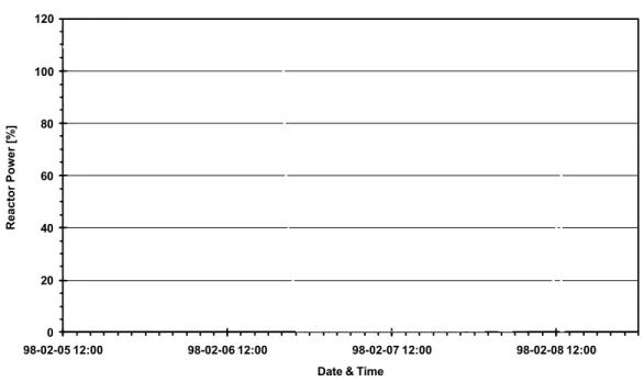
Oskarshamn-III - Power history 0 20 40 60 80 100 120 98-02-05 12:00 98-02-06 12:00 98-02-07 12:00 98-02-08 12:00 Date & Time
Reactor Power [%]
Figure 2-3: Oskarshamn-3 power history for the time period up to the scram.
The analysis (Post-Mortem-Reviewa (PMR) at the plant) of the event indicated that the overpower protection system was triggered and scrammed the reactor because of a strong and intense power oscillation in the core (see figure 2-4).
In figure 2-4, the measured APRM is plotted from the plant PMR-file. As can bee seen there are (in the plotted time interval) two occasions when the core is unstable.
From the PMR analysis there was pointed out that one main cause for the event could have been a transient on the feed-water supply but also outer causes. Conceivable causes/factors could have been:
• Disturbance in feed water supply (flow or temperature transient).
• The front-coupled automatic control system (reactor pressure) on the turbine governor valve could have caused amplification on the reactor power.
• Unfavorable core operation conditions (e.g. Xenon swing, Power distribution etc)
a
Process data are continuously stored on a so-called circular PMR file, and at the time for a scram the plant computer marks the time on the actual data point and starts collecting data for another couple of minutes. The contents of the PMR file (process data) represents in this way a specific time period before and after the event (scram). The PMR file contains besides the APRM power a large set of process data, so that these data can be used in PMR analysis to examine the main cause of the event.
As a part of the Swedish Nuclear Power Inspectorate (Statens kärnkraftinspektion, SKi) support on research in the area of power oscillation on the BWR, and to get a broader knowledge of the main reasons for the instability, Studsvik Scandpower (SSP) was assigned to investigate the Oskarshamn-3 (O3) event with the kinetic version of the nodal code SIMULATE-3 (SIMULATE-3K – S3K).
The assignment to SSP where as follows:
1. Set up an O3 data base so that an adequate investigation of the event can be done. 2. Examine and verify of the fuel and core loading at the time of the event.
3. Validate S3K against earlier stability measurements performed at O3. 4. Examine the oscillation event.
5. Perform a sensitive study to find the root causes. This report sums up the results from the points 3-5 above.
3 Validation of S3K
Based on the database of O3b, that was set up in this project, S3K has been validated against a set of stability measurements as follows, see table 3-1.
O3 stability measurements used for the S3K validation
Date/time Power % RC-flow % CRs inserted % Inlet- temp. Or enthalpy
911027/11:54 66.0 34.0 12.07 1168.0 kJ/kg 911027/13:46 69.6 33.0 11.69 1160.5 kJ/kg 911027/14:41 73.0 32.6 11.45 1156.9 kJ/kg 911027/17:14 69.3 33.0 12.07 1147.5 kJ/kg 911027/17:53 72.5 32.8 11.81 1142.6 kJ/kg 911027/18:45 61.9 29.6 13.04 1143.0 kJ/kg 911027/19:21 61.1 29.5 12.97 1142.6 kJ/kg 911027/20:36 72.2 37.5 12.17 1158.3 kJ/kg 911027/21:31 77.6 37.2 11.81 1152.6 kJ/kg 951007/08:45 63.4 34.0 8.44 266.6 C 951202/09:00 60.5 33.4 8.96 267.0 C 960913/19:40 62.7 33.3 8.58 266.6 C 970111/08:00 62.5 33.3 10.92 266.5 C 971205/19:45 65.3 36.6 4.58 268.0 C
Table 3-1: O3 stability measurements used for the S3K validation
Besides, the above measurements the SIMULATE-3K results from validation against the OECD/NEA Ringhals-1 stability benchmark have been referred to as reference and for comparison.
b
This file contains geometrical and some dynamic information, delivered from OKG - Oskarshamns Kraft Grupp AB (the operator of the Oskarshamn-3 NPP) and recalculated at Studsvik Scandpower AB to extend data for this project.
3.1 Definitions
Throughout this report definitions of decay ratio and frequency have been used as indicated in figure 3.1-1.
Definitions used in the analysis
42 43 44 45 46 0 2 4 6 8 10 12 Time (Second) Reactor Power (%) A1 A2 P
Decay Ratio = A2/A1 Frequency = 1/P
Figure 3.1-1: Definitions of decay ratio and frequency.
3.2 Validation results
The core conditions in the validation points cover a wide range of different operation conditions, but also a wide range of fuel types in the core.
The points from 911027 represent a core where the major part (62%) of the fuel is of older 8*8 design, and the later points (from 951007 and later) represent cores with more or less 100% of advanced 10*10 fuels.
The validation data include measurements from BOC (Beginning Of Cycle) and MOC (Middle Of Cycle) as well as measurements done at different Xenon conditions and different operating points (in the power/flow map).
Comparison of measured and S3K calculated result
Date/time Measuredc S3K Calculated
DR Frequency (Hz) DR Frequency (Hz) 911027/11:54 0.66 0.51 0.73 0.53 911027/13:46 0.80 0.50 0.84 0.52 911027/14:41 0.88 0.50 0.93 0.52 911027/17:14 0.85 0.50 0.86 0.53 911027/17:53 0.95 0.50 0.94 0.53 911027/18:45 0.89 0.47 0.88 0.49 911027/19:21 0.93 0.47 0.87 0.48 911027/20:36 0.71 0.54 0.78 0.57 911027/21:31 0.84 0.54 0.90 0.58 951007/08:45 0.72 0.52 0.78 0.56 951202/09:00 0.70 0.56 0.73 0.59 960913/19:40 0.68 0.51 0.76 0.54 970111/08:00 0.83 0.55 0.82 0.58 971205/19:45 0.69 0.51 0.74 0.58
Table 3.2-1: Comparison between measured and calculated results.
The above results give the following summary of statistic deviations for S3K (for all the cases):
Deviation between S3K and Measured values
Mean difference (S3K – Measured)
Standard deviation from mean difference.
Decay Ratio (DR) 2.9 % 4.1 %
Frequency (Hz) 2.8 % 1.3 %
Table 3.2-2: Statistic summary for S3K.
c
All the measured values of DR and Frequency are delivered from OKG and are results from noise analysis of the APRM signal with either AR (Auto Regressive method) or ARMA (Auto Regressive Moving Average method). In general, the analysis (independent of which method) has been done with a relatively low model order, in the range of 8 to 12.
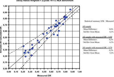
In figures 3.2-1 and 3.2-2 the results from S3K validation against the OECD/NEA Ringhals-1 Stability Benchmark problem are shown as a reference and for comparison (Lefvert T. 1996).
Decay Ratios Ringhals-1 (Cycles 14-17) NEA Benchmark
0,00 0,10 0,20 0,30 0,40 0,50 0,60 0,70 0,80 0,90 1,00 0,00 0,10 0,20 0,30 0,40 0,50 0,60 0,70 0,80 0,90 1,00 Measured DR Simulate-3K Calculated DR .
Statistical summary S3K - Measured
All sample
Mean Difference: 0,6% Std Dev from Mean: 6,1% All sample with measured DR > 0,50 Mean Difference: 0,2% Std Dev from Mean: 6,3% All sample with measured DR > 0,70 Mean Difference: 0,3% Std Dev from Mean: 5,2%
Figure 3.2-1: OECD/NEA Ringhals-1 Stability benchmark, comparison of decay ratio
(DR)
Resonance Frequency Ringhals-1 (Cycles 14-17) NEA Benchmark
0,00 0,10 0,20 0,30 0,40 0,50 0,60 0,70 0,80 0,90 1,00 0,00 0,10 0,20 0,30 0,40 0,50 0,60 0,70 0,80 0,90 1,00 Measured Frequency
Simulate-3K Calculated Frequency
Statistical summary S3K - Measured
All sample
Mean Difference: -0,1% Std Dev from Mean: 1,6%
Figure 3.2-2: OECD/NEA Ringhals-1 Stability benchmark, comparison of resonance
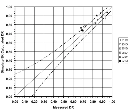
In figures 3.2-3 and 3.2-4 the results from table 3.2-1 are plotted. Evaluated DR Oskarshamn-III 0,00 0,10 0,20 0,30 0,40 0,50 0,60 0,70 0,80 0,90 1,00 0,00 0,10 0,20 0,30 0,40 0,50 0,60 0,70 0,80 0,90 1,00 Measured DR Simulate-3K Calculated DR 911027 11.54 - 21.31 951007 951202 960913 970111 971205 400 rpm curve S3K-beta KSEP = 46,0; TBARL = 0,8 'PER.OPT' 'ZBLK' 'STAT' 'OFF' 'OFF' 'ON'/
1/2 Core
Figure 3.2-3: Comparison of DR for validation points on O3
Evaluated Frequency Oskarshamn-III
0,00 0,10 0,20 0,30 0,40 0,50 0,60 0,70 0,80 0,90 1,00 0,00 0,10 0,20 0,30 0,40 0,50 0,60 0,70 0,80 0,90 1,00 Measured Frequency [Hz]
Simulate-3K Calculated Frequency [Hz]
911027 11.54 - 21.31 951007 951202 960913 970111 971205 400 rpm curve S3K-beta KSEP = 46,0; TBARL = 0,8 'PER.OPT' 'ZBLK' 'STAT' 'OFF' 'OFF' 'ON'/
1/2 Core
The dotted lines in both figures 3.2-1 and 3.2-3 represents the uncertainty (standard deviation) in the evaluation of the measured decay ratio (DR) (Lefvert T. 1996). Comparing the results from the O3 validation with OECD/NEA results shows that O3 results give a higher mean difference but a lower standard deviation.
Comparison between O3 and OECD/NEA results
O3 OECD/NEA
Mean difference DR 2.9 % 0.6 %
Standard deviation from mean-diff. DR 4.1 % 6.1 %
Mean difference frequency 2.8 % -0.1 %
Standard deviation from mean-diff. freq. 1.3 % 1.6 %
Table 3.2-3: Comparison of deviations for O3 and OECD/NEA validations
From table 3.2-3 it can bee seen that S3K for O3 has more or less a constant bias in both DR and frequency compared to the OECD/NEA benchmark. The bias magnitude for both DR and frequency is approximately +2.5%.
Without trying to quantify the reason for the higher deviation in the O3 cases compared to OECD/NEA result, the following causes can be mentioned that could contribute to this result:
• The OECD/NEA measured results are all determined with an ARMA method at a high model order, generally over 15.
• The O3 measured results are a mix of methods, AR and ARMA, at a low model order, generally lower than 12.
• For the early points (911027), the documentation on the operational condition is brief, with a limited amount of process log data.
• There is doubt about some of the reactor specific data used (geometrical and dynamic description) for which no references have been found.
• The process log data that have been used for all the cases are based on files of data where every time point in the files corresponds to a so-called on-line calculation in the core supervision system. The automatic on-line calculation is triggered every 0.5 hours, and besides this auto triggering manual requests can be made. The log data therefore represent the input condition (process data) for the corresponding on-line
• The “uncertainty band” (dotted lines) in figure 3.2-1 and figure 3.2-3 represents the uncertainty that is a result of using ARMA method with a model order of 20 to determine the measured DR. In the O3 case, the model order in the analyses of the measured data is low, which in general gives a slightly higher uncertainty.
Therefore, for O3 the “uncertainty band” should at least for lower DR be a somewhat wider.
From the comparison result for O3 it can be seen that S3K is capable with sufficient accuracy to be used for analysis of the instability event at Feb. 8, even if the results are not as good as those of the OECD/NEA Ringhals 1 benchmark.
4 Examination of the oscillation event
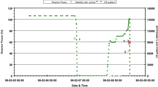
To be able to examine the oscillation event the operational history and conditions at actual points have been reconstructed. SIMULATE-3 has been used to follow in detail the operational history from Feb. 5 (equilibrium conditions at 109.3 % power) to the scram on Feb. 8. This core tracking reconstruction has been performed following the power/xenon transient (resulting from the shutdown on Feb. 6) and details in operating conditions. From this core tracking seven points have been saved for examination with S3K (see figures 4-1, 4-2 and 4-3).
Oskarshamn-III - Operating history
0 20 40 60 80 100 120 98-02-05 00:00 98-02-06 00:00 98-02-07 00:00 98-02-08 00:00 98-02-09 00:00 Date & Time
0 3000 6000 9000 12000 15000 18000
Reactor Power Stability calc.-points CR-pattern
3 - 7
2 1
Figure 4-1: Operating history from Feb. 5 to scram Feb. 8
The points # 1 to 7 have been selected from the process log data file (where an on-line case calculation has been performed) to be sure, that reliable process data are used. For point # 7 some extra data supplied from OKG (collected from the PMR file) have been used to be able to calculate the instability behavior as close as possible to the scram.
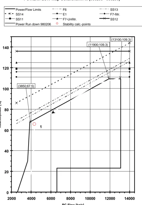
POWER/FLOW-map Oskarshamn-III (980205 - 980206) 0 20 40 60 80 100 120 140 2000 4000 6000 8000 10000 12000 14000 RC-Flow [kg/s] Power/Flow Limits F6 SS13 SS14 E1 F7-filtr. SS11 F7-Unfiltr. SS12
Power Run down 980206 Stability calc.-points
(3850;67.5)
(11900;109.3)
(13100;109.3)
1
Figure 4-2: Examination points # 1 at time for power run-down Feb. 6. Point # 1 represents a core situation at reduced power (in the same area in the
POWER/FLOW-map Oskarshamn-III (980208) 0 20 40 60 80 100 120 140 2000 4000 6000 8000 10000 12000 14000 RC-Flow [kg/s] Power/Flow Limits F6 SS13 SS14 E1 F7-filtr. SS11 F7-Unfiltr. SS12
Power Run up 980208 Stability calc.-points
(3850;67.5)
(11900;109.3)
(13100;109.3)
2 3 - 7
Figure 4-3: Examination points # 2 - 7 at time for power run-up Feb. 8.
Points #5 – 7 correspond to data that also could be plotted from the PMR-file. In figure 4-4 these points have been marked in the time scale of the PMR file data.
O-III APRM A Measured Reactor Power 980208 40 50 60 70 80 90 100 Analysis point # 5 Time 12.35 Analysis point # 6 Time 12.41 Analysis point # 7 Time 12.42
4.1 Results from examination points # 1 – 7
Tracking the power and xenon transient over the actual time span results in a core situation (regarding global Xenon and Iodine) as illustrated in figure 4.1-1.The axial power and xenon condition are plotted in figures 4.1-2 and 4.1-3.
Figure 4.1-1: Global Xenon and Iodine concentration during the transient
The stability response calculated with S3K using an automatic global perturbation on reactivity (reactor pressure ⇒ void reactivity feed back) gives the results for the points # 1 – 7 as listed in table 4.1-1.
SIMULATE-3K stability results for points # 1 – 7
Process data S3K-Calculated
Point # Power % Flow % CRs inserted % DR Frequency (Hz)
1 65.6 32.3 5.65 0.98 0.57 2 43.9 32.0 12.15 0.51 0.50 3 56.0 32.6 11.11 0.80 0.55 4 58.7 32.9 10.68 0.90 0.56 5* 57.9 31.8 10.64 0.92 0.55 6* 59.5 31.8 10.54 0.98 0.55 7* 60.5 31.8 10.35 1.02 0.56
* Points # 5 – 7 have the following measured DR and Frequency: # 5 (1.01,0.53), # 6 (0.98,0.53),
# 7 (1.06,0.53)d
Table 4.1-1: SIMULATE-3K stability results for points # 1 – 7
d
The measured values have been calculated with an ARMA method based on the PMR 5Hz sampled data.
As can be seen in table 4.1-1 points # 1, 6 and 7 have a clear tendency to be unstable. In figures 4.1-4 and 4.1-5 the stability responses for points # 1 - 7 have been plotted in the same manner as the case with power and xenon profiles in figure 4.1-2 and 4.1-3. In figures 4.1-4 and 4.1-5, the reactor power response (oscillation) after the perturbation is plotted (for the following 12 seconds) in the small boxes.
To summarize the results and visualize the operational conditions (power and flow) of the examination points the DR results are plotted in the power/flow maps in figure 4.1-6.
Detailed stability response results from points # 1 – 7 are presented in figure 4.1-7:1 – 4.1-7:7. As can be seen from these figures and from table 4.1-1 the examination points 1, 6 and 7 are more or less unstable with a DR very near 1.0. For point # 7 the
calculated DR is even > 1.0, and this means that the reactor power from period to period is increasing with a factor that is the same as the value for DR (1.02)e.
From the figures 4.1-4 to 4.1-7:7 it is clearly seen that the SIMULATE-3K results indicate that the stability behavior of the core was such during power run up that the DR is steadily increasing. Finally, at point # 7 the stability behavior (power oscillation) with SIMULATE-3K indicates that the power oscillation was amplified.
Oskarshamn-III - Power and Xenon Profile 0 20 40 60 80 100 120 98-02-05 00:00 98-02-06 00:00 98-02-07 00:00 98-02-08 00:00 98-02-09 00:00
Date & Time
Reactor Power [%] 0 3000 6000 9000 12000 15000 18000 CR-pattern [CR % Withdrawal]
Reactor Power Stability calc.-points CR-pattern
3 - 7 2 1 1,00 6,00 11,00 16,00 21,00 0 1 2
The solid line represents the axial Power profile and the dotted line represents the axial Xenon profile.
Oskarshamn-III - Power and Xenon Profile 30 40 50 60 70 80 90 12000 13000 14000 15000 16000 17000 18000
Reactor Power Stability calc.-points CR-Pattern
2
3 4 5 6
7
In the small boxes above: The solid lines represents the axial Power profiles and the
1,00 6,00 11,00 16,00 21,00 0 1 2 1,00E+00 6,00E+00 1,10E+01 1,60E+01 2,10E+01 0 1 2 1,00E+00 6,00E+00 1,10E+01 1,60E+01 2,10E+01 0 1 2 1,00 6,00 11,00 16,00 21,00 0 1 2 1,00E+00 6,00E+00 1,10E+01 1,60E+01 2,10E+01 0 1 2 1,00E+00 6,00E+00 1,10E+01 1,60E+01 2,10E+01 0 1 2
Oskarshamn-III - Stability analysis 0 20 40 60 80 100 120 98-02-05 00:00 98-02-06 00:00 98-02-07 00:00 98-02-08 00:00 98-02-09 00:00
Date & Time
0 3000 6000 9000 12000 15000 18000
Reactor Power Stability calc.-points CR-pattern
3 - 7 2 1 62 64 66 68 0 2 4 6 8 10 12
Oskarshamn-III - Stability analysis 30 40 50 60 70 80 90 12000 13000 14000 15000 16000 17000 18000
Reactor Power Stability calc.-points CR-Pattern
7 6 5 4 3 2 42 44 46 0 2 4 6 8 10 12 54 56 58 0 2 4 6 8 10 12 56 58 60 62 0 2 4 6 8 10 12 54 56 58 60 0 2 4 6 8 10 12 56 58 60 62 0 2 4 6 8 10 12 58 60 62 64 0 2 4 6 8 10 12
Oskarshamn-III - Stability evaluation Power Run Down 980206
40 45 50 55 60 65 70 75 3500 4000 4500 5000 RC Flow [kg/s] Reactor Power [%] Point # 1 DR = 0.98
Oskarshamn-III - Stability evaluation Power Run Up 980208 40 45 50 55 60 65 70 75 3500 4000 4500 5000 RC Flow [kg/s] Reactor Power [%] Point # 2 DR = 0.51 Point # 3 DR = 0.80 Point # 4 DR = 0.90 Point # 5 DR = 0.92 Point # 6 DR = 0.98 Point # 7 DR = 1.02
Instability respons at: 63 64 65 66 67 68 0 2 4 6 8 10 12 Time (Second) Reactor Power (%) Point 1 (980206 20.24) ============================================================= STABILITY EDIT
MEAN DECAY RATIO: 0.9826 MEAN PERIOD (S) : 1.7625 ST. DEV. DECAY RATIO: 0.0148 ST. DEV. PERIOD (S) : 0.0306
+---+---+---+---+---+ | SAMPLE | DECAY | PERCENT | PERIOD | PERCENT | | TIME (S) | RATIO | DEV. | (S) | DEV. | +---+---+---+---+---+ 4.000 0.997 1.453 1.750 -0.709 5.750 0.971 -1.181 1.750 -0.709 7.550 0.988 0.567 1.750 -0.709 9.300 0.974 -0.838 1.800 2.128 =============================================================
Simulate-3K Stability results
Figure 4.1-7:1: Stability result at point # 1
Instability respons at:
43 44 45 46 Reactor Power (%) Point 2 (980208 12.04) ============================================================= STABILITY EDIT
MEAN DECAY RATIO: 0.5143 MEAN PERIOD (S) : 2.0000 ST. DEV. DECAY RATIO: 0.0069 ST. DEV. PERIOD (S) : 0.0000
+---+---+---+---+---+ | SAMPLE | DECAY | PERCENT | PERIOD | PERCENT | | TIME (S) | RATIO | DEV. | (S) | DEV. | +---+---+---+---+---+ 4.100 0.507 -1.469 2.000 0.000 6.050 0.514 0.004 2.000 0.000 8.050 0.516 0.323 2.000 0.000 10.050 0.520 1.143 2.000 0.000 =============================================================
Instability respons at: 54 55 56 57 58 0 2 4 6 8 10 12 Time (Second) Reactor Power (%) Point 3 (980208 12.15) ======================================================== ===== STABILITY EDIT
MEAN DECAY RATIO: 0.8043 MEAN PERIOD (S) : 1.8125 ST. DEV. DECAY RATIO: 0.0221 ST. DEV. PERIOD (S) : 0.0306
+---+---+---+---+---+
| SAMPLE | DECAY | PERCENT | PERIOD | PERCENT |
| TIME (S) | RATIO | DEV. | (S) | DEV. |
+---+---+---+---+---+
Simulate-3K Stability results
Figure 4.1-7:3: Stability result at point # 3
Instability respons at:
56 57 58 59 60 61 0 2 4 6 8 10 12 Time (Second) Reactor Power (%) Point 4 (980208 12.23) ======================================================== ===== STABILITY EDIT
MEAN DECAY RATIO: 0.8979 MEAN PERIOD (S) : 1.8000 ST. DEV. DECAY RATIO: 0.0135 ST. DEV. PERIOD (S) : 0.0000
+---+---+---+---+---+
| SAMPLE | DECAY | PERCENT | PERIOD | PERCENT |
| TIME (S) | RATIO | DEV. | (S) | DEV. |
+---+---+---+---+---+
Simulate-3K Stability results
Instability respons at: 56 57 58 59 60 0 2 4 6 8 10 12 Time (Second) Reactor Power (%) Point 5 (980208 12.35) ======================================================== ===== STABILITY EDIT
MEAN DECAY RATIO: 0.9216 MEAN PERIOD (S) : 1.8250 ST. DEV. DECAY RATIO: 0.0214 ST. DEV. PERIOD (S) : 0.0354
+---+---+---+---+---+
| SAMPLE | DECAY | PERCENT | PERIOD | PERCENT |
| TIME (S) | RATIO | DEV. | (S) | DEV. |
+---+---+---+---+---+
Simulate-3K Stability results
Figure 4.1-7:5: Stability result at point # 5
Instability respons at:
59 60 61 62 Reactor Power (%) Point 6 (980208 12.41) ============================================================= STABILITY EDIT
MEAN DECAY RATIO: 0.9673 MEAN PERIOD (S) : 1.8125 ST. DEV. DECAY RATIO: 0.0263 ST. DEV. PERIOD (S) : 0.0306
+---+---+---+---+---+ | SAMPLE | DECAY | PERCENT | PERIOD | PERCENT | | TIME (S) | RATIO | DEV. | (S) | DEV. | +---+---+---+---+---+ 3.950 0.935 -3.320 1.850 2.069 5.750 0.976 0.854 1.800 -0.690 7.550 0.979 1.183 1.800 -0.690 9.350 0.980 1.282 1.800 -0.690 =============================================================
Instability respons at: 58 59 60 61 62 63 0 2 4 6 8 10 12 Time (Second) Reactor Power (%) Point 7 (980208 12.42) ======================================================== ===== STABILITY EDIT
MEAN DECAY RATIO: 1.0183 MEAN PERIOD (S) : 1.8000 ST. DEV. DECAY RATIO: 0.0103 ST. DEV. PERIOD (S) : 0.0000
+---+---+---+---+---+
| SAMPLE | DECAY | PERCENT | PERIOD | PERCENT |
| TIME (S) | RATIO | DEV. | (S) | DEV. |
+---+---+---+---+---+
Simulate-3K Stability results
Figure 4.1-7:7: Stability result at point # 7
4.2 Detailed examination of point # 7
A detailed examination has been performed of point # 7, in the way that the analyzing time in the calculation was unlimited. This leads to two different analyses of point # 7: 1. Simulation up to scram, where 97% reactor power had been used as a set point for
triggering the scram.
2. Simulation without scram, to analyze the situation if the scram had been delayed.
4.2.1 Simulation up to scram
The simulation up to scram is performed in such way that the power amplification is allowed to grow up to a set point value of 97% reactor power. When the simulated fission reactor power exceeds the set point value, SIMULATE-3K automatically
“scrams” the “calculation”. All the control rods at actual position are inserted in the core to fully inserted with a speed corresponding to 5 seconds for a full stroke. A general delay of 0.1 seconds has been used between “signal for scram” = exceeding 97% power and start of the control rod insertion.
In figure 4.2.1-1, the calculation is illustrated up to scram following the reactor power and control rod withdrawal.
Oskarshamn-III SCRAM simulation Point # 7 0 20 40 60 80 100 0 20 40 60 80 100 120 140 Time (Second)
Reactor Power (%) or CR % withdrawal
Power CR Group 1 to XX SCRAM Set-point
Figure 4.2.1-1: Simulation up to scram
In figures 4.2.1-2 and 4.2.1-3, detailed plots are shown for the time span from 110 seconds to scram.
Oskarshamn-III SCRAM simulation Point # 7
20 40 60 80 100
Reactor Power (%) or CR % withdrawal
Power CR Group 1 to XX SCRAM Set-point
Oskarshamn-III - 980208 Point # 7 Variation in Inlet Core Flow and Exit Dome Pressure
-600 -500 -400 -300 -200 -100 0 100 200 300 400 500 600 110 112 114 116 118 120 122 124 126 Time (Second)
Variation in Inlet Core Flow
(delta kg/s) -9,0 -7,5 -6,0 -4,5 -3,0 -1,5 0,0 1,5 3,0 4,5 6,0 7,5 9,0
Variation in Exit Dome Pressure
(delta kPa)
Inlet Flow Exit Pressure
Figure 4.2.1-3: Core flow and Exit pressure oscillations near scram
In the two figures above (4.2.1-2 and 4.2.1-3) the non-linear behavior of power and flow amplification when the DR > 1.0 is clearly seen.
In figures 4.2.1-1 and 4.2.1-2, it is clearly shown that the scram (even a short time after start of the scram) causes the oscillation to be completely suppressed.
Detailed examination of the axial power and void distributions for a whole oscillation cycle around time 125 seconds is shown in the following three figures (4 – 4.2.1-6). In these figures the axial distributions for core average and a hot channel are plotted.
Axial Relativ Power "SWING" Point # 7 at end of transient (at 125 second)
1 5 9 13 17 21 25 0,0 0,5 1,0 1,5 2,0 2,5 3,0 3,5 Relativ Power Node Min/Max Hot Channel Core Average
Axial power "SWING" Point # 7 at end of transient (at 125 second)
1 5 9 13 17 21 25 0,0 0,1 0,2 0,3 0,4 0,5 Nodal power (MW) Node Max hot Hot Channel Min hot Max ave Core Average Min ave
Total Core Power (MW)
Min Value = Max Value =
1130,8 2935,3
Figure 4.2.1-5: Absolute axial power “swing”
In the figure above the maximum nodal power “swing” in the hot channel is showed to be more or less 0.25 MW for one oscillation cycle. For the core average power, the same value is about half of that for the hot channel.
Axial Void "Swing" Point # 7 at end of transient (at 125 second)
1 5 9 13 17 21 25 -10% 0% 10% 20% 30% 40% 50% 60% 70% 80% 90% 100% Void Node Min/Max Hot Channel Core Average Hot-Diff Core-Diff
To be able to correlate some of the interesting core dynamic parameters these have been plotted together in figure 4.2.1-7:
• Total Power (% Rated) = Fission power in %
• Coolant Power (% Rated) = Fission power deposited in the coolant in % (rated maximum power =109.3% or 3300 MW)
• Inlet and Outlet Flow (% Rated) = Inlet and Outlet flow into and out from the core in % of 13100 kg/s (maximum flow)
• Reactivity in $
Titel: Title Skapad av:
The AthenaTools Plotter Widget Set Version 6.0 Förhandsgranska:
Den här EPS-bilden sparades inte med en inkluderad förhandlsgranskning. Beskrivning:
Den här EPS-bilden kan skrivas ut på en PostScript-skrivare, men inte på andra typer av skrivare.
4.2.2 Simulation without scram
In this section, we have postulated that the scram for some reason would be delayed or that SS14 would not be triggered (single failure). To be able to do that we allow SIMULATE-3K to follow (in the calculation) the oscillation beyond the scram triggering point. From the calculated results, we can try to find out:
• What is the maximum power and reactivity release if the scram had been delayed?
It should be noted that this kind of calculation could have a high degree of uncertainty!
In figure 4.2.2-1 it can be noticed that the power oscillation finally reaches so-called “limit cycle” oscillation with a maximum change of power and reactivity. In figure 4.2.2-1 the calculation indicates that limit cycle is reached within a few tens seconds after the scram time.
Oskarshamn-III - 980208 Point # 7 Reactor Power [%] and Reactivity [$]
0 20 40 60 80 100 120 0 50 100 150 200 Time (Second) Reactor Power [%] -1,0 -0,8 -0,6 -0,4 -0,2 0,0 0,2 0,4 0,6 Reactivity [$]
Scram Power % Reactivity ($)
Detailed examination of the limit cycle oscillation is shown in figure 4.2.2-2, and summarized in the table below.
Reactor power and reactivity during limit cycle
Limit cycle Minimum Maximum
Reactor power [%] 35 103
Reactivity [$]f -0.80 +0.41
Table 4.2.2-1: Reactor power and reactivity during limit cycle
Oskarshamn-III - Limit Cycle Oscillation Reactor Power [%] and Reactivity [$]
30 40 50 60 70 80 90 100 110 180 190 200 Time (Second) Reactor Power [%] -1,0 -0,8 -0,6 -0,4 -0,2 0,0 0,2 0,4 0,6 Reactivity [$] Power % Reactivity ($)
Figure 4.2.2-2: Limit cycle oscillation
As indicated in the introduction to this section and pointed out in the figures 4.2.2-1 and 4.2.2-2 this kind of calculation (limit cycle) is affected with a high degree of
uncertainty.
$ = Fraction of realized reactivity compared to the total amount of reactivity in the delayed neutrons.
β ρ = $ Reactivity
5 Sensitive study to find the root causes.
The root cause of the event can be found in one of the following two areas:
1. Impact or amplification from auxiliary or external systems, that could feed back (triggering or maintaining) an instability event.
2. The situation in the core itself, with a naturally high potential to be unstable. In the following chapters, we will try to find out which of the above two areas that could be blamed as the root cause for the event.
5.1 Influence from external system or external loop.
Referring to the results in chapter 3 and 4 (with overall good agreement with measured values) it is obvious that the root cause of the instability event on February 8, 1998, could be focused on the second item in the preamble of chapter 5.
To furthermore confirm the conclusion that the situation in the core itself is the root cause to the instability event, optional SIMULATE-3K calculations have been made without any feed back from the outer circulation loop in the reactor. In this way, we can examine the situation in the core without impact from the outer loop.
In the figure 5.1-1 the results from two calculated options are plotted: Option:
• Peripheral system “OFF” = The outer loop to the core is replaced by constant boundary conditions. This results in a calculation with no dynamic feedback from the outer loop (downcomer, RC pump etc.).
• Peripheral system “ON” = Ordinary calculation where the outer loop is modeled with plant specific input and is an integrated part in the calculation, which results in dynamic feedback to the core. This option has been used for all the results in the report except for those in this subchapter (5.1).
From the figure 5.1-1 it is clearly seen that points # 5, 6 and 7 follow the general bias of 0.1 – 0.2 in DR (O3 validation data, see chapter 3) between the two calculation options. It can also be seen that points # 5, 6 and 7 have high (the highest) DR values from the calculations with the peripheral system “OFF”.
The high values for points # 5, 6 and 7 indicate clearly that the core itself has a potential to get unstable and that the root cause of the event has to be found in the core situation itself. For that reason, it is natural to focus on the power distribution in the core.
DR comparison PERIPHERAL SYSTEM "OFF" and "ON" 0,00 0,10 0,20 0,30 0,40 0,50 0,60 0,70 0,80 0,90 1,00 1,10 0,00 0,10 0,20 0,30 0,40 0,50 0,60 0,70 0,80 0,90 1,00 1,10 Option PERIPHERAL SYSTEM "OFF"
Option PERIPHERAL SYSTEM "ON"
O-3 Validation data Point # 5 Point # 6 Point # 7 400 rpm curve S3K-beta KSEP = 46,0; TBARL = 0,8 'PER.OPT' 'ZBLK' 'STAT' 'OFF' 'OFF' 'ON'/
1/2 Core
Figure 5.1-1: DR comparison from different calculations options
As always, when there is a core instability situation, where the root cause is in the core itself, the main reason can be found in the so-called “flow/flux” relation, where:
• Flow = Core coolant flow (%)
• Flux = Reactor power (%) (Neutron flux)
A low value of “flow/flux” (below ∼0.5) is always a potential “area” in the power flow map where instability can occur. To avoid instability during operation with low value on flow/flux, it is of major importance that the power distribution in the core is such that it will not destabilize the core. In this situation, the following operating parameters have a major impact on the power distribution in the core:
• Inlet temperature and/or flow variation to the core:
Disturbance of feed water flow or temperature, RC pump flow transients.
• Radial and axial power distribution: Control rod pattern, Xenon transient etc.
From the PMR data from Oskarshamn-3 we could see that there has been a feed water disturbance (in between point # 5 and 6), a start-up of one more feed water pump following ordinary routines and instructions. This small disturbance could explain the sudden change in stability behavior, but not the general high DR for the points # 5, 6 and 7.
In the successive subsections of chapter 5 sensitive studies in the following areas described:
• Impact from Xenon transient
5.2 Impact from Xenon transient
From figure 4.1-1 we could see that the xenon concentration in the core is in a transient change for the points # 2 – 7. The Xenon contribution to instability can mainly be coupled to the axial transient changes. In the right hand diagram of figure 4.1-1, we can see that the Xenon Axial Off-Set (Xenon-AO) is more or less the same as for the calculated point # 1.
Although the Xenon-AO is the same between point # 1 and 7, it is still possible that the distribution and the global value of Xenon could have impacted the stability behavior. To investigate the impact from Xenon a calculation with SIMULATE-3 has been performed producing an operating point # 8, which has been created by conserving the operational conditions from point # 7 (as is) + 96 hours exposure. With this calculation, point # 8 will have an equilibrium Xenon concentration with the rest of the core
operating data the same as in point # 7 (CR-pattern, Inlet flow, Inlet temperature). Performing a SIMULATE-3K calculation on point # 8 gives then the Xenon impact on the stability behavior of the core.
Oskarshamn-III - Power Profile
20 30 40 50 60 70 80 90 98-02-08 00:00 98-02-09 00:00 98-02-10 00:00 98-02-11 00:00 98-02-12 00:00 98-02-13 00:00
Date & Time
Reactor Power [%]
Reactor Power Stability calc.-points Constant Operation Conditions
The stability calculation point "8" have been constructed with constant operation
condition "as is" in point "7" + 96 hours depletion to reach XENON equilibrium
7 8 1 , 0 0 E + 0 0 6 , 0 0 E + 0 0 1 , 1 0 E + 0 1 1 , 6 0 E + 0 1 2 , 1 0 E + 0 1 0 1 2 1 , 0 0 E + 0 0 6 , 0 0 E + 0 0 1 , 1 0 E + 0 1 1 , 6 0 E + 0 1 2 , 1 0 E + 0 1 0 1 2
In the small boxes above:
The solid lines represents the axial Power profiles and the dotted lines represents the axial Xenon profiles.
Oskarshamn-III - Stability analysis 20 30 40 50 60 70 80 90 98-02-08 00:00 98-02-09 00:00 98-02-10 00:00 98-02-11 00:00 98-02-12 00:00 98-02-13 00:00
Date & Time
Reactor Power [%]
Reactor Power Stability calc.-points Constant Operation Conditions
7
8
The stability calculation point "8" have been constructed with constant operation
condition "as is" in point "7" + 96 hours depletion to reach XENON equilibrium 5 8 6 0 6 2 6 4 0 2 4 6 8 1 0 1 2 5 8 6 0 6 2 6 4 0 2 4 6 8 1 0 1 2
Figure 5.2-2: DR sensitivity study from xenon distribution
Instability respons at:
58 59 60 61 62 63 0 2 4 6 8 10 12 Time (Second) Reactor Power (%) Point 8 (980212 12.42) ======================================================== ===== STABILITY EDIT
MEAN DECAY RATIO: 0.9979 MEAN PERIOD (S) : 1.8250 ST. DEV. DECAY RATIO: 0.0243 ST. DEV. PERIOD (S) : 0.0354
+---+---+---+---+---+
| SAMPLE | DECAY | PERCENT | PERIOD | PERCENT |
| TIME (S) | RATIO | DEV. | (S) | DEV. |
+---+---+---+---+---+
Simulate-3K Stability results
Figure 5.2-3: Stability result at point # 8
In the figures above it is shown that the xenon distribution has no major impact in this case. The DR only changes from 1.02 (point # 7) to 1.00 (point # 8), and therefore we can finally determine that the xenon (lack of and distribution) has no significant impact on the stability behavior of the coreg.
g
NB!
This conclusion is only valid for this core operational condition! In addition, the conclusion can not be used as a general confirmation for xenon’s impact on stability behavior!
5.3 General power distribution
One of the final operational items is the general power distribution of the core; we want to find out if this distribution can be blamed for the high decay ratio. Examining the power distributions, we find the following general features:
1. An average axial power profile with accentuated bottom peaked power. 2. A high degree of “Double-Humped” axial power profile.
3. Local areas with very highly bottom peaked power.
4. The high powered bottom peaked areas are not just separate from each other, but they are also well isolated by deeply inserted control rods (in between those areas). All four items (each by itself or in combination) is from experience known to
destabilize the core (D’Auria F. et.al., 1997).
In figure 4.2.1-4 (chapter 4.2.1), the axial power profile from point # 7 is plotted. This profile, besides the bottom peaked power, also shows clearly the double humped axial distribution, and the accentuated bottom peaked power in the hot channel. From this, it is easy to understand that there are regions in the core with highly bottom peaked power.
To be able to see and visualize both the radial and axial power distributions in the core the 2D Axial off-set Power Product (2APP) distribution is created:
i i
i Power AxialOff-Set Channel 2DRelativePower Fraction Channel APP
2 = ×
With this distribution, positive values indicate a top displaced channel power and vice versa, a negative value indicates a bottom displaced channel power.
In figure 5.3-1 below from point # 7 the radial 2APP map shows clearly (blue areas) where the bottom pronounced regions are located, and that those regions are radially well separated.
To investigate the sensitivity on DR for changes of the axial and radial power
distribution we change the control rod pattern at point # 7 by just insert 4 manoeuvre groups of CRs to shallow positions (85% withdrawal). The original CR pattern and the adjusted (shallow rods) pattern are shown in figure 5.3-2 below.
Original CR pattern at point # 7
18 6 50 6 18 6 6 50 6 6 6 6 6 50 6 6 18 6 50 6 18
Adjusted CR pattern at point # 7
85 18 6 50 85 85 85 6 18 6 6 85 85 50 85 6 6 85 6 85 6 6 85 50 85 85 6 6 18 6 85 85 85 50 6 18 85
---The values in the figures above represent the single CR withdrawal in percent. “---“ represents the value 100% withdrawn. The “Bold” values in the lower pattern represent the four manoeuvre group (4*4 CR:s) that have been inserted in shallow positions (85% withdrawal).
Figure 5.3-2: Original and adjusted CR patterns at point # 7
Comparison of decay ratios from the two above cases (original CR pattern vs. adjusted CR patterns) is summarized in table 5.3-1 below.
Comparison of Decay Ratio
Case point # 7 Decay Ratio (DR)
Original CR pattern 1.02
Adjusted CR pattern 0.84
The difference in radial and axial power distributions between the two cases is illustrated in figure 5.3-3. It can be seen from figure 5.3-3 that the shallow CRs force the average power towards the top (smearing) of the core and redistribute the radial power from the center. In combination, this gives a more homogeneous power distribution in the core and therefore a lower decay ratio.
Figure 5.3-3: Impact on radial and axial power distributions from insertion of shallow
CRs
In figure, 5.3-3 we can see that the “double-humped” axial power profile is almost eliminated by the use of shallow CR:s.
5.4 Conclusions
The results in chapter 4 and the sensitivity study in chapter 5 can briefly be summarized in the following conclusions:
• Point # 1, 5,6 & 7, all with different power distributions and CR patterns and with no reported or logged disturbances from the auxiliary/external systems, all show high values of decay ratio (> 0.9).
• In between points #5 and 6, a small disturbance in feed water supply is noticed from the PMR file data (start up of one more feed water pump following the ordinary routines and instructions). This results in a small disturbance in moderator level at time (approximately) 140 seconds, which gets the core to amplify. At time 220 seconds, (approximately) the feed water was back to normal, which caused the amplification to be suppressed. This small and not unusual disturbance in feed water supply (when starting an extra pump) could not have caused the core to amplify without a general high DR.
• Comparison of decay ratio results from the two calculational options in SIMULATE-3K indicates that points # 5, 6 & 7 have high decay ratio values (around 0.8 or higher), without feed back from the outer thermo hydraulic loop (calculation option "OFF"). This indicates that the core itself (without any external feed back or interference) has all necessary properties to get unstable.
• No significant contribution from non-equilibrium Xenon effects to the decay ratio could be noticed.
• There is a strong dependency of the decay ratio on the axial and radial power distribution in the core.
• By inserting a small number of shallow CRs the decay ratio could be decreased by some two tenths of a DR unit (from around 1.0 to around 0.8).
Taking all the above aspects into account one can draw the conclusion that the main reason for the instability event was an unfortunate combination of core design and control rod patterns, resulting in isolated regions of the core with strongly bottom peaked power and double-humped axial distributions.
6 References
Lefvert T., RINGHALS 1 STABILITY BENCHMARK Final Report, NEA/NSC/DOC(96)22,
NEA Nuclear Science Committee, Nuclear Energy Agency Organisation for Economic Co-Operation and Development, November 1996.
D’Auria F. et al., STATE OF THE ART REPORT ON THE BOILING WATER
REACTOR STABILITY [SOAR ON BWRS], General Distribution OCDE/GD(97)13,