Published under the CC-BY4.0 license
Open reviews and editorial process: Yes
Preregistration: No Analysis reproduced by: Jack Davis All supplementary files can be accessed at OSF: https://doi.org/10.17605/OSF.IO/C4WN8
Cumulative Science via Bayesian Posterior Passing:
An introduction
Charlotte O. Brand
University of Exeter, Penryn Campus, College of Life and Environmental Science
James P. Ounsley
University of St Andrews, School of Biology
Daniel J. van der Post
University of St Andrews, School of Biology
Thomas J.H. Morgan
Arizona State University, School of Human Evolution and Social Change
This paper introduces a statistical technique known as “posterior passing” in which the results of past studies can be used to inform the analyses carried out by subsequent studies. We first describe the technique in detail and show how it can be implemented by individual researchers on an experiment by experi-ment basis. We then use a simulation to explore its success in identifying true parameter values compared to current statistical norms (ANOVAs and GLMMs). We find that posterior passing allows the true effect in the population to be found with greater accuracy and consistency than the other analysis types con-sidered. Furthermore, posterior passing performs almost identically to a data analysis in which all data from all simulated studies are combined and analysed as one dataset. On this basis, we suggest that posterior passing is a viable means of implementing cumulative science. Furthermore, because it prevents the ac-cumulation of large bodies of conflicting literature, it alleviates the need for tra-ditional meta-analyses. Instead, posterior passing cumulatively and collabora-tively provides clarity in real time as each new study is produced and is thus a strong candidate for a new, cumulative approach to scientific analyses and pub-lishing.
Keywords: Bayesian statistics, metascience, cumulative science, replication crisis, stereotype threat, psychological methods
The past two decades have seen a great increase in the study of the scientific process itself, a field dubbed ‘metascience’ (Munafo et al. 2017). The growth of this field has been driven by a series of re-sults that question the reliability of science as it is currently practiced. For instance, in 2015 a global
collaboration of scientists failed to replicate 64 of 100 findings published in top psychology journals in 2008 (Open Science Collaboration 2015). Given this, many scientists have turned their efforts towards identifying potential improvements to the scientific process.
A key focus within metascience is how to im-prove the use of statistical methods and the pro-cess of scientific publishing. Problems such as p-hacking, “HARKing” and the “file-drawer” effect have been discussed in science for many years with mixed opinions and widespread debate (e.g. Bissell 2013; Bohannon 2014; Kahneman 2014; Schnall 2014; Fischer 2015; Pulverer 2015). Recent proposals such as guidelines against the mis-use of p-values (Wasserstein & Lazar 2016), banning the p-value (Trafimow & Marks 2015), statistical checking software (Epskamp & Nuijten, 2016), rede-fining statistical significance (Benjamin et al., 2018), justifying your alpha (Lakens et al., 2018), pre-registering methods (Chambers et al. 2014; van ’t Veer & Giner-Sorolla, 2016) and the Open Sci-ence movement generally (e.g. Kidwell et al. 2016) are propagating discussion and endorsement of substantial changes to scientific publishing and research methods.
One indication of the current scientific practice underperforming is the presence of large numbers of publications presenting conflicting conclusions about the same phenomenon. This is the case, for instance, in the ‘stereotype threat’ literature, in which experiments are designed to “activate” a neg-ative stereotype in participants’ minds, and this leads to reduced performance in participants for which the stereotype is relevant. A common ques-tion is whether being told that women typically per-form worse than men at mathematical or spatial tasks depresses the performance of female partici-pants on these tasks (e.g. Flore & Wicherts 2015). De-spite the seemingly straight-forward nature of this question, and the publication of over 100 papers on this topic, there are no clear conclusions about the veracity of stereotype threat.
Traditionally, meta-analyses are conducted to clarify the existence of a purported effect in the erature. This is also true of the stereotype threat lit-erature, which includes seven meta-analyses (Wal-ton & Cohen 2003; Nguyen & Ryan 2008; Wal(Wal-ton & Spencer 2009; Stoet & Geary 2012; Picho, Rodriguez & Finnie 2013; Flore & Wicherts 2014; Doyle & Voyer 2016). However, in many cases meta-analyses do not lead to increased certainty (Ferguson 2014; Lakens et al., 2017; Lakens, Hilgard, & Staaks, 2016). One rea-son is that meta-analyses are not just used to deter-mine whether an effect truly exists but can also be used to reveal the underlying causes of variation
across studies. Consequently, meta-analyses often differ in their interpretations of the literature, de-pending on the specific question that the authors are interested in. Moreover, in some cases meta-analyses can actually increase uncertainty. For in-stance, they can uncover evidence of publication bias (as is the case with four of the stereotype threat meta-analyses), or researcher effects, both of which undermine the credibility of individual studies. More generally, the lack of objective inclusion criteria can render the conclusions of meta-analyses just as fraught as the results of individual studies. An exam-ple of this is seen in the ‘cycle shift’ debate, which asks whether women’s mate preferences change over their ovulatory cycle. Here, an initial meta-analysis argued against the existence of an effect, only to be followed by another meta-analysis that found the exact opposite to be the case (Gildersleeve, Haselton, & Fales, 2014a, 2014b; Wood, Kressel, Joshi, & Louie, 2014). Despite both being based on the aggregation of a large number of stud-ies (many of which were included in both meta-anal-yses) one meta-analysis must be wrong. Given these difficulties, meta-analyses do not provide an unam-biguous solution for resolving conflicted literatures.
Meta-analyses are not the only way to mathe-matically combine the results of multiple studies. Many recent proposals fall within the category of “cumulative science”, a process in which each study incorporates prior work into its analyses. For this reason, each study can be considered a meta-analy-sis of sorts, with its conclusions reflecting the data collected both in that study as well as prior studies. As such, there is no need for traditional meta-anal-yses in a cumulative science framework. One exam-ple of cumulative science is the use of Sequential Bayes Factors, which can be used to update the ex-tent to which evidence is weighted in favour of the presence of an effect based on new data (Schönbrodt, Wagenmakers, Zehetleitner, & Peru-gini, 2017). Similarly, ‘Curate Science’, and measures of replication success, have gained support (LeBel, Vanpaemel, Cheung, & Campbell, 2018; Zwaan, Etz, Lucas, & Donnellan, 2017). Here, we describe and test another approach to cumulative science, “pos-terior passing”, which is a straightforward extension of Bayesian methods of data analysis. In what follows we first cover Bayesian inference, which is the the-oretical background of posterior passing. We then describe how posterior passing can be implemented
in practice. Finally, using the case study of stereo-type threat mentioned above, we use a simulation to compare the ability of traditional analytic tech-niques and posterior passing to correctly identify effects of different sizes (including 0). We demon-strate that, given a representative number of studies characteristic of the stereotype threat literature, posterior passing provides an up-to-date, accurate estimation of the true population level effect with-out the need for a dedicated meta-analysis. Con-versely, using traditional analytic techniques such as ANOVAs in “one-shot” analyses, produced an abun-dance of conflicting effect size estimates as is found in the stereotype threat literature at present. Fur-thermore, posterior passing produces almost iden-tical results to a ‘meta’ GLMM analysis in which all available data were combined and analysed as one dataset.
Bayes Rule and Posterior Passing
Bayes’ theorem (a.k.a. Bayes’ rule), is a method of assigning probabilities to hypotheses. Given a set of competing hypotheses and our beliefs about how likely they are to be true, it provides us with the probability that each hypothesis is true when we collect more data. More formally this can be written as:
𝑝(ℎ|𝑑) =𝑝(ℎ)𝑝(𝑑|ℎ) 𝑝(𝑑)
where p(h|d) is the probability that each hypoth-esis is true taking the data into account (the “poste-rior”), p(h) is the probability of each hypothesis be-ing true prior to collectbe-ing data (the “prior”), and
p(d|h) is the probability that each hypothesis would
have produced the observed data (the “likelihood”). The denominator, p(d), can be conceptualized as the probability of getting the data under any hypothesis, but in practice it acts as a normalizing constant to ensure that the posterior probabilities sum to 1. To illustrate the application of Bayes theorem we will now walk through a simple example based on a thought experiment used by the 16th century statis-tician Jacob Bernoulli. Other introductions to Bayes-ian inference can be found elsewhere (van de Schoot et al. 2014; Morgan, Laland & Harris 2014; McElreath 2016, Kruschke 2011) and we encourage readers to
seek these out.
Consider an urn containing a mix of blue and white pebbles and imagine we are interested in un-derstanding what proportion of the pebbles are blue. To start with, we have two competing hypoth-eses: (1) 75% of the pebbles are blue, or (2) 75% of the pebbles are white (we assume that these are the only two possibilities). We will test these hypotheses by collecting data; three times we will draw a pebble from the urn, note its color, and replace it. Before collecting data, let us note our prior beliefs (p(h) in the above equation). Without any knowledge we could assign each hypothesis equal prior probability (i.e. 50% in both cases) but let us imagine we have reason to suspect hypothesis 2 is more likely (per-haps we know blue pebbles are rare, or we know that the urn was filled at a factory that produces more white than blue pebbles, or maybe someone told us that they glanced inside the urn and it looked mostly white etc.). Given this we assign prior probabilities of 0.4 and 0.6 to the two hypotheses.
Now to data collection; let us assume we happen to draw three blue pebbles. We need to use this data to calculate the likelihood for each hypothesis, i.e. the probability of drawing three blue pebbles under each hypothesis (p(d|h) in the above equation). The probability of drawing a blue pebble three times un-der hypothesis 1 is 0.753 , and 0.253 under hypothesis 2. This is 0.42 and 0.016 respectively. Note that the likelihood is much higher for hypothesis 1, this means that the data are more consistent with hy-pothesis 1 than with hyhy-pothesis 2 and so we should expect Bayes’ theorem to shift the probabilities of each hypothesis in favor of hypothesis 1.
The next step is to calculate the normalizing constant, p(d), which is the probability of getting the data under any hypothesis. It is the sum of the prob-ability of getting the data under each hypothesis multiplied by the prior probability that each hypoth-esis is true, i.e. it is the sum of the likelihoods multi-plied by the priors. In our case we only have two hy-potheses, so p(d) is p(h1)p(d|h1) + p(h2)p(d|h2). We now have all the necessary parts to execute Bayes’ rule and we can calculate the probability that each hy-pothesis is true. The table below summarizes this process, showing that because the data were more consistent with hypothesis 1 it is now the more likely of the two hypotheses, even though it started with a lower prior probability.
This example can also illustrate how Bayes’ theo-rem facilitates cumulative science. Assume someone else decides to draw more pebbles from the same urn. How can they include our data in their anal-yses? The solution is straightforward: they simply need to use our posterior as their prior. More gen-erally, by using the posterior from a previous study as the prior in the next one, the posterior of the sec-ond study will reflect the data collected in both studies, forming a chain of studies each of which builds on the last to provide an increasingly precise understanding of the world. This method is referred to as “posterior passing” (Beppu & Griffiths 2009) and is the focus of this manuscript. If posterior pass-ing is effectively implemented, it is mathematically equivalent to collecting all the data in a single high-power study (Beppu & Griffiths 2009). In both a the-oretical analysis and a lab experiment, Beppu and Griffiths (2009) found that posterior passing led to successively better inferences over time. Given this, posterior passing may offer a valuable addition to the scientific process, with particular benefits for fields suffering from ambiguous literatures or repli-cation crises. The passing of posteriors across stud-ies not only incorporates information from prior studies, but also prevents any experimental dataset from carrying too much weight. In the next section we discuss how posterior passing can be imple-mented as part of the Bayesian analysis of data.
Posterior passing in practice
While the above example is much simpler than most scientific problems, it is relatively straightfor-ward to generalize the theory to continuous hy-pothesis spaces as is characteristic of much scien-tific research. For instance, say we are hypothesiz-ing about the value of a parameter in a model. Rather than assigning prior probabilities to specific hypoth-eses (such as “the parameter is 2.5”) we describe a probability density function across the range of pos-sible values for the parameter. For instance, if we have reason to believe the parameter is close to 10, we might use a normal distribution with a mean of 10 and standard deviation of 1 (this permits any value from positive to negative infinity, but 10 is the single most likely value and 95% of the probability mass falls between 8 and 12). The likelihood, too, becomes a function over the hypothesis space and the nor-malizing constant is calculated the same way as be-fore: the prior is multiplied by the likelihood and the resulting function is summed across the hypothesis space. The posterior, again calculated as the prior multiplied by the likelihood and divided by the nor-malizing constant, is also a probability density func-tion, allocating posterior probability over the pa-rameter space which can then be passed as the prior in subsequent studies.
The application of Bayes’ rule to continuous hy-pothesis spaces (such as in parameter estimation) runs into problems, however, because it is often im-possible to calculate the normalizing constant. The
Table 1. A summary of the example execution of Bayes’ theorem. The probability that each hypothesis is true, taking the data into account (the “posterior”, column 5), is the prior (column 2) multiplied by the likelihood (column 3) and divided by a normalizing constant (the sum of column 4).
Hypothesis Prior, p(h) Likelihood,
p(d|h) Prior * Likelihood, p(h)p(d|h) Posterior, p(h|d)
1 0.4 0.42 0.17 0.95
circumnavigation of this problem relied on the de-velopment of modern computers and new tech-niques such as Markov Chain Monte Carlo (MCMC) methods. The details of this technique are compli-cated (for accessible introductions to MCMC see McElreath 2016; Kruschke 2011), but it works by providing the user with a series of values (called “samples”) that approximate values drawn from the posterior probability density function even though the exact density function itself remains unknown.
As the number of samples approaches infinity, statistical descriptions of the samples converge on
the same values of the posterior probability density function itself. For instance, the mean of the samples approaches the mean of the posterior probability density function, and an interval that contains 95% of the samples will also contain 95% of the probabil-ity mass of the posterior distribution. So, even though the posterior probability density function technically remains unknown, we can nonetheless describe it in a variety of ways.
In order to implement posterior passing we now need a means by which samples from the posterior can be translated into a probability density function
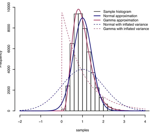
samples Frequency −2 −1 0 1 2 3 4 0 2000 4000 6000 8000 10000 Sample histogram Normal approximation Gamma approximation Normal with inflated variance Gamma with inflated variance
Figure 1. The translation of a histogram of samples into a probability distribution. Here the samples (black histogram of 50,000 samples) look somewhat normal, but they are all positive and the histogram is positively skewed. Using the mean and variance to define a normal distribution (solid blue lines, scaled x10000) produces a reasonable fit, but the lower tail places non-zero probability density on negative values while the peak appears to be slightly higher than the peak of the histogram. Using a gamma distribution instead (solid red line) produces a perfect fit. Artificially inflating the variance (dashed lines) changes the distributions. In the case of the normal distribution it greatly widens it, placing increasing amount of probability mass below 0. In the case of the gamma distribution the positive skew grows, but all the probability mass remains above 0. In this way the variance is increased but the mean of the probability distribution remains the same as the mean of the samples.
that will be the prior in subsequent studies. The sim-plest approach is to assume the posterior is mally distributed and then define the prior as a nor-mal distribution with the same mean and standard deviation as the samples generated. So, if the mean of the samples is 5.3 and the standard deviation is 0.8, then this can be assumed to correspond to the probability distribution N(5.3, 0.8). However, assum-ing normality could lead to an inaccurate descrip-tion of the posterior. To alleviate this concern re-searchers can inflate the standard deviation of the passed posterior, for instance changing N(5.3, 0.8) to
N(5.3, 8). This will broaden the prior, effectively
weakening its influence and so avoiding distorting results due to the posterior passing process. By the same token, however, broadening the prior will also lessen the influence of past research and potentially slow down scientific accumulation.
A more nuanced approach is to build bespoke priors for each set of posterior samples. The re-searcher can choose a probability distribution that closely matches the shape of the posterior samples (e.g. normal, exponential, gamma or beta) and ap-propriate parameter values can be calculated from the samples. For instance, a normal distribution with the same mean and standard deviation as the sam-ples, or a gamma distribution with shape and rate parameters calculated from the mean and variance of the samples. As before, if the researcher wishes to err on the side of caution by weakening the effect of the passed posterior on subsequent analyses they need to simply inflate the variance of the distribu-tion. Figure 1 shows an example of this in action il-lustrating that a highly suitable distribution is de-rived in this manner. Inflating the uncertainty in the prior also facilitates posterior passing in cases where there are differences in experimental design or analytic technique. Even within a single area of research it is rare that any two studies are exactly the same. These differences mean that the posterior produced by one study may not be entirely appro-priate for the prior in another. However, experi-ments do not have to be identical to engage in pos-terior passing: as long as they are addressing the same theoretical “effect” then there is reason to draw on previous knowledge. In these cases, the un-certainty in the posterior should be inflated to ac-count for differences in experimental design.
Another possibility is that the prior could be based on a previous study that used non-Bayesian
methods. If even a point estimate for the effect size is given then this can be used as the mean of the prior with the variance set to a suitable value corre-sponding to the researcher level of uncertainty. Pre-cisely how much a prior should be watered down in cases such as these will depend on the similarity of the studies in question and discussion of this should be an important part of the peer-review and publi-cation process. Moreover, where concerns are raised, robustness analyses can be used in which the prior is varied and the resultant effect on the con-clusions described and discussed. In the short term, it may be beneficial to compare results with and without posterior passing to show the difference in inference that results from either approach.
The simulation
In this section we present a simulation of the sci-entific process, testing the hypothesis that posterior passing will benefit science relative to other meth-ods of data analysis and avoid the accumulation of large, ambiguous literatures. We simulate a series of experiments testing for an interaction between two variables. We vary (i) the true effect size of the in-teraction, (ii) the scale of between individual differ-ences and (iii) the statistical technique employed by scientists. The simulation is, in part, based on the stereotype threat literature as this produced an am-biguous and conflicted literature, as discussed pre-viously. As such, we refer to the interacting variables as sex and condition, and various simulation param-eters (e.g. the number of participants per study) are set to values representative of the stereotype threat literature.
We use the simulation to compare four different analysis methods; an analysis of variance (ANOVA), a generalised linear mixed model (GLMM), a Bayesian GLMM using MCMC estimation (henceforth “BGLMM") and a Bayesian GLMM using MCMC esti-mation and posterior passing (henceforth “PP”). ANOVAs have been widely used in psychology for decades and still represent one of the most com-monly used analytic approaches (including for stud-ies of stereotype threat), despite suggestions of their inadequacy for many types of experimental de-sign (Jaeger 2008). A move towards using general-ised linear mixed models for categorical and bino-mial data has been suggested as more appropriate
than methods often used by psychologists and ecol-ogists (Jaeger 2008; Bolker et al. 2009) and so we in-clude both a frequentist GLMM and a Bayesian equivalent. Finally, we include “posterior passing” (Beppu & Griffiths 2009) to examine whether imple-menting posterior passing as a form of cumulative knowledge updating would be beneficial. Addition-ally, we performed a single BGLMM analysis over all simulated datasets combined (henceforth “meta BGLMM") in order to compare posterior passing against the best possible scenario of a single high-power study.
Each repeat of the simulation involved the fol-lowing three steps: 1) a population of one million po-tential experimental subjects was created, 2) 60 se-quential experiments were carried out, each involv-ing 80 participants takinvolv-ing part in 25 experimental trials (numbers chosen as representative of the ste-reotype threat literature) and 3) the 60 datasets were analysed using the four different analysis methods. For each combination of parameter values, we carried out 20 repeat simulations. Further details are given below, and full model code is available at
www.github.com/thomasmorgan/posterior-pass-ing.
Population Creation
Each of the 1,000,000 simulated participants is defined by two values; their sex (0 or 1, with half of the population having each value) and their perfor-mance at the experimental task relative to the pop-ulation average (positive values indicate above aver-age performance, and negative values below averaver-age performance). Each participant’s performance value was drawn randomly from a normal distribution with mean 0 and with variance that varied across simulations (from 0 to 1 in steps of 0.25). For each participant there was another participant of the same sex but with the opposite performance value, and another of the opposite sex, but with the same performance value. This ensured that the average performance value in the population was exactly 0 (equivalent to 50% success on a binary choice trial), and the variation in performance within each sex was equal.
Data Collection
Datasets were generated by randomly selecting a sample of 80 individuals who were then split into a control group and an experimental group (20 of each sex in each group). Each simulated participant was presented with 25 binary-choice trials and the num-ber of trials they answered correctly was generated by sampling from a binomial distribution in which the likelihood of success per trial was:
𝑝(= 𝑙𝑜𝑔𝑖𝑠𝑡𝑖𝑐(𝑝𝑒𝑟𝑓𝑜𝑟𝑚𝑎𝑛𝑐𝑒(+ 𝑒 ∗ 𝑐𝑜𝑛𝑑𝑖𝑡𝑖𝑜𝑛(∗ 𝑠𝑒𝑥() where e is the unknown interaction effect that the simulated experiments are attempting to iden-tify. In the context of stereotype threat, it can be considered as the magnitude of the effect of the ste-reotype threat condition on the behaviour of women (i.e. participants of sex 1). Note that participants of sex 0 (i.e. men) are insensitive to condition, and con-dition 0 (the control concon-dition) does not affect par-ticipant behaviour.
Across simulations, we consider five different values for e (the magnitude of the effect in question): 0, 0.5, 1, 1.5 and 2. Given that the average population performance was 0 (equivalent to a 50% chance of success per trial) these values increase the average probability of success from 0.5 to 0.5, 0.62, 0.73, 0.82 and 0.88 respectively. Thus, the cases we explored range from no interaction effect, up to a large effect, exceeding the effect sizes reported in meta-anal-yses of the stereotype threat literature (e.g. Doyle & Voyer 2016).
Data Analysis
We performed four methods of analysis on each simulated dataset. The first is the predominant method of analysis used in the stereotype threat lit-erature; analysis of variance (2 x 2 ANOVA). Average success on the task (i.e. number of successes/num-ber of trials) was subjected to a 2(Sex) x 2(Condition) ANOVA, that included a main effect of sex, a main effect of condition, and an interaction between sex and condition at a significance value of p<0.05.
The second method is a generalised linear mixed model (GLMM) which models number of successes as a binomially distributed variable and uses a logit
link function. The same outcome and predictor var-iables are used as in the ANOVA (i.e. a baseline effect, and effects of sex and condition as well as a sex*condition interaction), but a random effect for participant is implemented. This method fits param-eters based on a maximum likelihood approach and estimates the linear effect that our manipulation and independent variables have on the log odds of suc-cess in any given trial.
The third approach uses the same model formu-lation as the GLMM, but uses Bayesian MCMC meth-ods to generate parameter estimates in JAGS. Mini-mally informative priors (normal distributions with mean 0 and precision 0.01) were used for all param-eters, and so we expect that the outcomes of this analysis should be extremely similar to that of the frequentist GLMM.
The fourth approach is a Bayesian GLMM with “posterior passing,” (Beppu & Griffiths 2009) in which the prior for e (the interaction effect) is based
on the posterior from the most recent previous ex-periment. As a deliberately coarse implementation of posterior passing we assumed the posterior was normal and defined it solely by its mean and preci-sion.
Results
Within each simulation, the general pattern was for posterior passing to converge on the true effect size while the other analysis types produce a series of independent results distributed stochastically around the true value with no convergence over time (see Fig. 2A and 2B). Five metrics were used to more thoroughly examine the performance of each analytic technique across simulations, 1) the average point estimate; 2) the true positive rate; 3) the false positive rate; 4) the average width of the 95% confi-dence/credible interval; and 5) the average differ-ence between the effect estimate and the true value. Figure 2. Analysis estimates produced from a single simulation of 60 experiments. The true effect sizes (displayed by the horizontal black line) are (a) 0 and (b) 2 (equivalent to an increase in the probability of responding correctly of 0.38). In both cases there is no individual variation. Across experiments, the estimates produced by the ANOVA, GLMM and BGLMM vary stochastically around the true population average, with the accuracy or certainty of each analysis unrelated to its position in the series. Furthermore, in panel (b) the ANOVA estimates are considerably less certain than those of the GLMM or bGLMM. In contrast to all other methods considered, posterior passing allows the analysis to become more accurate and more certain over time. Note that a particularly skewed data set (data set 9, in panel a) prompts all analyses to find a positive result, despite this, posterior passing is nonetheless able to correct itself by the end of the simulation.
These were calculated for the analysis of each sim-ulated data set, except in the case of posterior pass-ing where only the final analysis in each simulation was used. This is because, with posterior passing, in-formation from each dataset is incorporated into subsequent analyses and so the final analysis con-tains information from all 60 datasets.
Effect size estimates
All analysis types were generally effective at esti-mating the size of the effect (see Fig. 3). However, as the between-individual variation increases, the ANOVA underestimates the effect size to a modest extent.
True positive result rates
For all analyses, the ability to detect a positive ef-fect increased with the true efef-fect size (Fig. 4). How-ever, for the ANOVA, GLMM and BGLMM increasing individual variation decreased the true positive re-sult rate. With posterior passing, there is no such ef-fect; positive results are likely to be found whenever the true effect is non-zero
Figure 3. Average effect size estimates from the five analysis types over 20 simulations of 60 datasets (Bayesian GLMM not shown as it is identical to the GLMM). The true population average is on the x axis, and the individual variation on the y axis. Colour corresponds to effect size estimate according to the key to the right of the panels.
False positive result rates
When the true effect was 0, all analyses were un-likely to produce (false-)positive results but did oc-casionally do so (see Fig. 4). Across all datasets (N=6000) the ANOVA produced 304 false positives (5.1%, close to the expected false positive rate of 5%), the GLMM 341 false positives (5.7%) and the BGLMM 304 false positives (5.1%). For posterior passing (and the meta BGLMM), we are concerned only with whether the final analysis in each series produced a false-positive result. Over 100 simulations in which the true effect size was zero (i.e. 20 repeats of 5 dif-ferent variance levels), posterior passing produced
two false positives, while the meta BGLMM pro-duced one.
Uncertainty
In general, the width of the 95% confi-dence/credible intervals (henceforth “uncertainty”) decreases with the true effect size, but increases with individual variation (Fig. 5). There are differ-ences between analyses however. The ANOVA is much more sensitive to individual variation than to the true effect size, i.e. increasing the true effect size only modestly reduces uncertainty, while in-creasing individual variation greatly increases un-certainty. Both the GLMM and BGLMM produce Figure 4. Positive rate for the five analysis types over 20 simulations of 60 datasets (Bayesian GLMM not shown as it is identical to the GLMM). The size of the true population average is on the x axis, and the individual variation on the y axis. Colour gives the positive result rate, ranging from 0 - 1, according to the key to the right of the panels. An analysis finds a positive effect in the population if the upper and lower bounds for its 95% confidence/credible interval do not include zero, the proportion of analyses in which a positive effect is found is the positive results rate.
confident results provided either the true effect size is high or individual variation is low, however if the effect size is small, but variation high, then model estimates are highly uncertain. Finally, while the un-certainty of both PP and the combined BGLMM is sensitive to the effect size and individual variation, it is only minimally so and confidence is very high across all of the parameter space we explored. The meta BGLMM, in which all data are analysed in a sin-gle analysis, performs almost identically to posterior passing.
Error
The average difference between the parameter estimates and the parameter’s true value was very low across all of the parameter combinations we
considered, except in the case of the ANOVA (Fig.6). This is because the ANOVA systematically underes-timates the value of the parameter when the true population average is high and individual variation is high (see Fig. 6).
Discussion
This paper introduces posterior passing; a statis-tical technique, based on Bayes’ Theorem, that uses the results of prior studies to inform future work. In this way it allows the operationalization of cumula-tive science, allowing individual studies to build on each other, avoiding conflicted literatures and Figure 5. Analysis uncertainty measure for the five analysis types as a function of true population average and individual variation (Bayesian GLMM not shown as it is identical to the GLMM). Colour represents the uncertainty of each analysis as given by the key to the right of the panels.
thereby reducing the need for dedicated meta-anal-yses. To test the performance of posterior passing we conducted a simulation of datasets sampled from populations with varying effect sizes. Different sta-tistical techniques were used to analyse the datasets and compared to a posterior passing approach over the same datasets. We found that although no method was perfect (e.g. all methods produced a non-zero number of false-positive results), poste-rior passing leads to greater certainty over time about the existence and size of an effect compared with the other statistical methods considered. As such this work supports the proposal that posterior passing is a viable means by which cumulative sci-ence can be implemented.
One of the goals of this project was to test whether posterior passing could effectively identify the true value of an effect in a context where other
analytic techniques have led to the build-up of an ambiguous literature, such as that concerning ste-reotype threat. Such literatures are defined by a mix of positive and negative findings, and in practice they have remained ambiguous despite multiple meta-analyses. In our simulations, examination of the positive result rate shows that such ambiguity is common to all non-cumulative analyses when be-tween individual variation is high and when the ef-fect size is small. Nonetheless, posterior passing is highly successful at correctly identifying the effect-size in these cases (only 2% of simulations produced a false-positive result).
These findings have important implications for the way scientists conduct, analyse and publish their research. Firstly, the use of ANOVAs (the current norm in priming studies) is shown to be particularly problematic. In our results, the ANOVA was the least Figure 6. Analysis estimate error as a function of true population average and individual variation (Bayesian GLMM not shown as it is identical to the GLMM) . Colour gives the size of the error, ranging from -0.1 to 0.1, according to the key to the right of the panels.
accurate at identifying the effect size, especially when the effect size was small and the variation high. The priming literature is precisely when re-searchers predict effect sizes to be small and indi-vidual variation to be high, as the mechanism under-lying the effect is unknown and some individuals are expected to be more or less susceptible to the effect depending on various moderating variables (see Bargh 2012; Gelman 2016). Therefore, the fact that ANOVAs are less likely than other methods to be able to accurately decipher an effect in these types of datasets suggests that researchers studying priming effects (as well as other small, variable ef-fects) should move away from the ANOVAs and on to other methods, as has been previously suggested (e.g. Jaeger 2008).
A second implication of our results is that poste-rior passing is considerably better than using Bayes-ian methods per se. With minimally informative pri-ors, the Bayesian GLMM did not provide any detect-able improvement in performance compared to the frequentist GLMM. This was expected because the important difference between the GLMM and the Bayesian GLMM was the use of priors, but by using minimally informative priors we masked this differ-ence. This might appear to suggest that there is little benefit to using Bayesian methods over frequentist methods if priors are implemented uninformatively. However, other benefits exist that are not consid-ered in our simulation. For instance, the philosophy of Bayesian inference is arguably more intuitive than null hypothesis significance testing (McElreath 2016), with Bayesian credible intervals more readily understood than frequently misinterpreted p-val-ues and confidence intervals (Belia, Fidler, Williams, & Cumming, 2005; Greenland et al., 2016). Nonethe-less, bearing these other benefits in mind, our sim-ulation results clearly suggest that posterior passing is a major benefit to using a Bayesian approach.
Reassuringly, even our deliberately coarse imple-mentation of posterior passing (in which only the posterior for the interaction term was passed, and it was assumed to be normal) was highly successful. Moreover, even when spurious results are present (e.g. Fig.2a, dataset 9), posterior passing rapidly re-verts to the true population effect. As a measure of the success of posterior passing we compared it to a single, “meta”, Bayesian GLMM conducted over all 60 datasets combined, as this is equivalent to the greatest possible performance achievable through
posterior passing. According to all of our metrics for evaluating the performance of different analytic techniques, posterior passing was virtually indistin-guishable from this ‘meta Bayesian GLMM’. None-theless, further work could measure the effect of more refined implementations of posterior passing (including passing all parameters) as this may accel-erate the convergence of knowledge concerning the effects in question.
Posterior passing is not the only means to achieve cumulative science, however, and, as men-tioned in the introduction, Sequential Bayes Factors and Curated Replications hold similar promise. Our results cannot comment on the efficacy of these methods relative to posterior passing, however, there are some key differences between the ap-proaches. First, the use of Bayes Factors is not un-controversial and their application has been debated elsewhere (e.g. Robert, 2016). One such argument is that Bayes Factors retain the “accept/reject” philos-ophy of null hypothesis significance testing, whereas other researchers have called for a shift to-wards more accurate parameter estimation and model comparison approaches (Cumming, 2013; McElreath, 2016). We agree with the sentiment of Schönbrodt and colleagues (2017) that estimation and hypothesis testing answer different questions and have separate goals, reflected by a trade-off be-tween accuracy and efficiency respectively. We ar-gue that ultimately scientists should value both ac-curacy and efficiency, but not prioritise efficiency at the expense of accuracy. Furthermore, posterior passing offers a means of achieving both accurate and (more) efficient estimates than the other analy-sis techniques included in our simulation, as poste-rior passing converges on the correct effect size within 10-15 analyses (compared to the full 60 da-tasets). With regards to Curated Replications and calls for measures of replication success (LeBel et al., 2018; Zwaan et al., 2017), these approaches can be distinguished from posterior passing in that they formalize the process of replication to ensure the robustness of findings. Posterior passing, con-versely, does away with the notion of replications as studies build on each other rather than specifically testing the results of prior studies.
Despite its success in our simulation, posterior passing is unlikely to be a scientific cure-all. One factor identified as a problem in science, but not considered in our simulation, is publication bias (the
increased likelihood of publishing positive findings compared to null findings). It is likely that the per-formance of posterior passing, along with the other analyses considered, will be negatively affected by publication bias. Indeed, posterior passing may ex-acerbate the problem of publication bias if research-ers only put forward their positive results to be part of a posterior passing framework. That said, if avail-able data from multiple studies are put towards a cumulative analysis, regardless of their novelty, re-searchers may be more motivated to publish their null results, as well as replications, and so the imple-mentation of posterior passing may reduce publica-tion bias indirectly. Given these uncertainties, it would be valuable for further work to ascertain how sensitive each analysis type is to various levels of publication bias.
Another assumption of our simulation is that all analyses are similar or comparable enough to use in a posterior passing framework. In actual scientific practice, however, scientists may struggle to use the results of one analysis to inform the next one due to differences in experimental design or analytic model structure. Moreover, even where a single model structure is agreed this may systematically differ from reality, introducing bias into model estimates. Further work is needed to explore the effects of this kind of mismatch on the performance of posterior passing. Nonetheless, as previously discussed, pos-teriors can be watered down by increasing their var-iance, thereby lessening the effect of prior work on current findings. While such practice necessarily slows down scientific accumulation, it will reduce the risks that inter-study incompatibilities pose to posterior passing. This highlights how appropriate use of priors will be an important issue for research-ers, as well as editors and reviewresearch-ers, and that it is important that manuscripts make clear which priors were used and why. Researchers may also wish to include robustness checks in which priors are mod-estly adjusted and the subsequent change in results included in supplementary materials.
In this manuscript, we have presented posterior passing as one way in which cumulative science can be implemented. Among the benefits of posterior passing is that it is easy to implement as a simple ex-tension beyond standard Bayesian analyses of data. Moreover, our simulations suggest that posterior passing works well in contexts where traditional,
non-cumulative, analyses produce conflicting re-sults across multiple studies. The use of posterior passing in these contexts would potentially identify the true effect with confidence, and without relying on meta-analyses that, in practice, often fail to re-solve debates. Nonetheless further work is needed to evaluate posterior passing, in particular, how well it fares when faced with other known problems in science, such as biases in publication.
Open Science Practices
This article earned the Open Data and the Open Materials badge for making the data and materials available. It has been verified that the analysis repro-duced the results presented in the article. The entire editorial process, including the open reviews, are published in the online supplement.
References
Bargh, J.A. (2012). Priming Effects Replicate Just Fine,
Thanks. Psychology Today. from:
www.psychologytoday.com
Belia, S., Fidler, F., Williams, J., & Cumming, G. (2005). Researchers misunderstand confidence intervals and standard error bars. Psychological
methods, 10(4), 389.
Benjamin, D. J., Berger, J. O., Johannesson, M., Nosek, B. A., Wagenmakers, E. J., Berk, R., ... & Cesarini, D. (2018). Redefine statistical
significance. Nature Human Behaviour, 2(1), 6. Beppu, A., & Griffiths, T. L. (2009). Iterated learning
and the cultural ratchet. In Proceedings of the
31st annual conference of the cognitive science society (pp. 2089-2094). Austin, TX: Cognitive
Science Society.
Bissell, M. (2013). Nature Comment: Reproducibility: The risks of the replication drive. Nature, 503, 333-334.
Bohannon J. (2014) Replication effort provokes praise—and ‘bullying’ charges. Science. 2014; 344:788–789.
Bolker, B. M., Brooks, M. E., Clark, C. J., Geange, S. W., Poulsen, J. R., Stevens, M. H. H., & White, J. S. S. (2009). Generalized linear mixed models: a practical guide for ecology and
evolution. Trends in ecology & evolution, 24(3), 127-135.
Chambers, C. D., Feredoes, E.,
Muthukumaraswamy, S. D., & Etchells, P. (2014). Instead of" playing the game" it is time to change the rules: Registered Reports at AIMS Neuroscience and beyond. AIMS
Neuroscience, 1(1), 4-17.
Cumming, G. (2013). Understanding the new
statistics: Effect sizes, confidence intervals, and meta-analysis. Routledge.
Doyle, R. A., & Voyer, D. (2016). Stereotype
manipulation effects on math and spatial test performance: A meta-analysis. Learning and Individual Differences, 47, 103-116.
Epskamp S, Nuijten MB. statcheck: Extract
statistics from articles and recompute p values. R package version 1.0.1.
http://CRAN.R-project.org/package=statcheck2015.
Ferguson, C. J. (2014). Comment: Why meta-analyses rarely resolve ideological debates. Emotion Review, 6(3), 251-252.
Fischer, M. R. (2015). Replication–The ugly duckling of science? GMS Z Med Ausbild, 32, 5.
Flore, P. C., & Wicherts, J. M. (2015). Does stereotype threat influence performance of girls in stereotyped domains? A meta-analysis. Journal of School Psychology. Gelman, A. (2016, Feburary 12). Priming Effects
Replicate Just Fine, Thanks. from
www.andrewgelman.com/2012
Gildersleeve, K., Haselton, M. G., & Fales, M. R. (2014). Do women’s mate preferences change across the ovulatory cycle? A meta-analytic review. Psychological Bulletin, 140(5), 1205. Gildersleeve, K., Haselton, M. G., & Fales, M. R. (2014). Meta-analyses and p-curves support robust cycle shifts in women’s mate
preferences: Reply to Wood and Carden (2014) and Harris, Pashler, and Mickes (2014).
Greenland, S., Senn, S. J., Rothman, K. J., Carlin, J. B., Poole, C., Goodman, S. N., & Altman, D. G. (2016). Statistical tests, P values, confidence intervals, and power: a guide to
misinterpretations. European journal of
epidemiology, 31(4), 337-350.
Jaeger, T. F. (2008). Categorical data analysis: Away from ANOVAs (transformation or not) and towards logit mixed models. Journal of memory
and language, 59(4), 434-446.
Kahneman, D. (2014). A new etiquette for replication. Social Psychology. 45, 310–311 Kidwell, M. C., Lazarević, L. B., Baranski, E.,
Hardwicke, T. E., Piechowski, S., Falkenberg, L. S., ... & Errington, T. M. (2016). Badges to acknowledge open practices: a simple, low-cost, effective method for increasing transparency. PLoS Biol, 14(5), e1002456. Kruschke, J. (2011). Doing Bayesian data analysis: A
tutorial with R, JAGS, and Stan. Academic
Press.
Lakens, D., Adolfi, F. G., Albers, C. J., Anvari, F., Apps, M. A., Argamon, S. E., ... & Buchanan, E. M. (2018). Justify your alpha. Nature Human
Behaviour, 2(3), 168.
Lakens, D., Hilgard, J., & Staaks, J. (2016). On the reproducibility of meta-analyses: Six practical recommendations. BMC psychology, 4(1), 24. Lakens, D., LeBel, E. P., Page-Gould, E., van Assen,
M. A. L. M., Spellman, B., Schönbrodt, F. D., … Hertogs, R. (2017, July 9). Examining the Reproducibility of Meta-Analyses in Psychology. Retrieved from osf.io/q23ye LeBel, E. P., McCarthy, R., Earp, B. D., Elson, M., &
Vanpaemel, W. (2018). A Unified Framework To Quantify The Credibility Of Scientific
Findings. OpenLeBel, Etienne P et al.“A Unified
Framework to Quantify the Credibility of Scientific Findings”. PsyArXiv, 13.
McElreath, R. (2016). Statistical rethinking: A Bayesian course with examples in R and Stan (Vol. 122). CRC Press.
Morgan, T. J., Laland, K. N., & Harris, P. L. (2015). The development of adaptive conformity in young children: effects of uncertainty and consensus. Developmental science, 18(4), 511-524.
Munafò, M. R., Nosek, B. A., Bishop, D. V., Button, K. S., Chambers, C. D., du Sert, N. P., ... &
Ioannidis, J. P. (2017). A manifesto for reproducible science. Nature Human Behaviour, 1, 0021. Chicago.
Nguyen, H. H. D., & Ryan, A. M. (2008). Does stereotype threat affect test performance of minorities and women? A meta-analysis of experimental evidence. Journal of Applied
Psychology, 93(6), 1314.
Open Science Collaboration. (2015). Estimating the reproducibility of psychological science.
Science, 349(6251), aac4716.
Pulverer, B. (2015). Reproducibility blues. The EMBO
journal, 34(22), 2721-2724.
Picho, K., Rodriguez, A., & Finnie, L. (2013). Exploring the moderating role of context on the mathematics performance of females under stereotype threat: A meta-analysis. The
Journal of social psychology, 153(3), 299-333. Robert, C. P. (2016). The expected demise of the
Bayes factor. Journal of Mathematical
Psychology, 72, 33-37
Schnall, S. (2014). Clean data: Statistical artifacts wash out replication efforts. Social Psychology, 45(4), 315-317
Schönbrodt, F. D., Wagenmakers, E. J., Zehetleitner, M., & Perugini, M. (2017). Sequential hypothesis testing with Bayes factors: Efficiently testing mean differences. Psychological Methods, 22(2), 322.
Stoet, G., & Geary, D. C. (2012). Can stereotype threat explain the gender gap in mathematics performance and achievement? Review of General Psychology, 16(1), 93
Trafimow, D, Marks, M. (2015). Editorial. Basic and
Applied Social Psychology, 37(1),1-2.
van de Schoot, R., Kaplan, D., Denissen, J., Asendorpf, J. B., Neyer, F. J., & Aken, M. A. (2014). A gentle introduction to Bayesian analysis: applications to developmental research. Child development, 85(3), 842-860. van't Veer, A. E., & Giner-Sorolla, R. (2016).
Pre-registration in social psychology—A discussion and suggested template. Journal of
Experimental Social Psychology, 67, 2-12.
Wasserstein, R. L., & Lazar, N. A. (2016). The ASA's statement on p-values: context, process, and purpose. The American Statistician.
Walton, G. M., & Cohen, G. L. (2003). Stereotype lift. Journal of Experimental Social
Psychology, 39(5), 456-467.
Walton, G. M., & Spencer, S. J. (2009). Latent ability grades and test scores systematically
underestimate the intellectual ability of negatively stereotyped students. Psychological
Science, 20(9), 1132-1139.
Wood, W., Kressel, L., Joshi, P. D., & Louie, B. (2014). Meta-analysis of menstrual cycle effects on women’s mate preferences. Emotion
Re-view, 6(3), 229-249.
Zwaan, R. A., Etz, A., Lucas, R. E., & Donnellan, M. B. (2017). Making replication mainstream.