2016:39 Recommended residual stress profiles for stainless steel pipe welds

(1)

Research

Recommended residual stress profiles

for stainless steel pipe welds

2016:39

Author: Etienne Bonnaud Jens Gunnars

(2)

(3)

SSM perspective

Background

SSM and the Swedish nuclear power plant owners have financed Inspecta Technology in Sweden to analyze stainless steel pipe welds to obtain good estimations of weld residual stress (WRS) distributions. Detailed knowledge of the residual stress field in different types of welds is impor-tant since they can have subsimpor-tantial influence on degradation mecha-nisms such as stress corrosion cracking and fatigue. Residual stresses also have to be considered when assessing safety margins for failure by fracture.

Objective

The primary objective has been to update the recommended weld resid-ual stresses for stainless steel pipe butt-welds, based on new knowledge on heat source modelling, material properties for high temperatures and material constitutive modeling.

Results

Recommended through-thickness weld residual stress distributions have been developed. Detailed numerical welding simulations have been per-formed by using 2-dimensinal finite element technique for a set of cases covering most stainless steel pipe welds in Swedish nuclear power plants, together with sensitivity studies with respect to material modelling, pipe geometry and heat input.

Best-estimate typical data have been used for influencing parameters with the aim to establish realistic through-thickness stress distributions to be applied in structural integrity assessments, especially for stress corrosion crack growth.

Recommended residual stresses are presented along paths in the center line of the weld and in the heat affected zones. The recommended stress profiles are given as polynomials for each analyzed weld case. For inter-mediate geometries it is recommended to apply linear interpolation. Compared to earlier recommendations the axial residual stress profiles generally show a stronger trend for sinus type distributions.

Need for further research

There is a need for further developments for weld residual stresses for weld joints which differ from the ones studied in this report. There is also a need for more work regarding 3-dimensional effects, for example when repair welds are made for part of the pipe circumference

Project information

Contact person SSM: Björn Brickstad Reference: SSM2013-2202

(4)

(5)

2016:39

Authors: Etienne Bonnaud, Jens Gunnars Inspecta Technology AB, Stockholm

Recommended residual stress

(6)

This report concerns a study which has been conducted for the Swedish Radiation Safety Authority, SSM. The conclusions and view-points presented in the report are those of the author/authors and do not necessarily coincide with those of the SSM.

(7)

Recommended residual stress profiles

for stainless steel pipe welds

Summary

Residual stresses in stainless steel pipe butt-welds have been analyzed by numerical weld simulation, taking into account recent develop-ments within heat source modelling and material modelling for weld-ing simulation. Recommended through-thickness weld residual stress distributions have been developed by analysis of cases covering a large set of austenitic piping, together with sensitivity studies. Typical data have been applied for influencing parameters, with the aim to establish realistic stress distributions.

Recommended residual stresses are presented along paths in the cen-ter line of the weld and in the heat affected zones. In section 6 of the report the recommended stress profiles are given as polynomials for each analyzed weld case. For intermediate geometries it is recom-mended to apply linear interpolation.

(8)

1 Background

Detailed knowledge of the residual stress field in different types of welds is important since they can have substantial influence on degra-dation mechanisms as stress corrosion cracking and fatigue. Weld residual stresses has a large influence on the behavior of cracks that possibly could occur during normal operation. Residual stresses also have to be considered when assessing safety margins for failure by fracture. Further, crack opening can be affected by residual stresses, which may be important to consider for non-destructive testing or in assessment of leak rate detection.

Welding processes are complex and involves localized heating with high thermal gradients, deposition of molten filler material, successive weld passes that affect earlier deposited material. The weld and base material undergo complex thermo-mechanical cycles involving elas-tic, plaselas-tic, creep and viscous deformation. These processes result in residual stresses and strains and modify material properties. The weld may also interact with other welds and undergo subsequent processing which also affects the final residual stress field. Examples of this are post-weld heat treatments, pressure tests and operational transients. Fracture mechanical defect tolerance analyzes are performed with postulated cracks when developing inspection programs. Defect toler-ance analyzes are also used if a defect is discovered during inspection, to assess whether safety margins are met for additional operation. Re-sidual stresses are needed as input when establishing inspection pro-grams with the purpose to detect any cracks well before they threaten safety. Thus, accurate prediction of the magnitude and distribution of residual stresses at welds is important in order to arrive at proper con-clusions.

Damage tolerance analyzes for the Swedish nuclear power plants are performed in accordance to the fracture mechanical handbook [1] which also include recommended residual stress profiles. The earlier recommendations for residual stresses are based on analysis per-formed 1996-1999 [2,3,4]. During the last decade there have been major developments both within calculation and measurement of re-sidual stresses. Several projects have been performed for development and validation of weld residual stress prediction [5,6,7,8,9,10]. This has resulted in improved numerical procedures, heat source modelling and material modelling. These projects show that the earlier recom-mendations in [1] for residual stress profiles need to be updated in accordance to new knowledge.

(10)

assumptions are applied also for the residual stress distributions, this results in very high crack growth rates and very short inspection inter-vals. This differs noticeably from the experiences and can result in improper prioritization of preventive efforts. For this reason the aim is to establish more realistic residual stress profiles.

This project has the purpose to update the recommended weld residual stresses for stainless steel pipe butt-weld, based on new knowledge within heat source modelling, material properties for high tempera-tures and material constitutive modeling. Realistic through-thickness residual stress distributions are developed by detailed numerical weld-ing simulations, usweld-ing typical data for influencweld-ing parameters. The residual stress profiles are self-balancing distributions for the axial stresses. Validation to measurements is performed for some available cases. Sensitivity analyses are performed for realistic variations and selected recommendations are based on results that imply the fastest crack growth from the pipe inside. The recommended residual stress profiles are developed with current knowledge and efforts to represent realistic residual stress distributions for stainless steel pipe welds.

(11)

2 Scope

This project provides an update for recommended weld residual stresses for stainless steel pipe butt-welds found in the Swedish nucle-ar power plants (NPPs). Realistic through-thickness residual stress distributions are developed by detailed numerical welding simulations, using typical data for influencing parameters. The recommendations are based on new knowledge within welding heat source modeling and materials modeling.

Finite element based weld residual stress modeling is performed for different thicknesses, together with sensitivity analyses. An overview of the geometries analyzed is presented in Table 1. Thicknesses cov-ered are from 6 mm to 65 mm, and the pipe geometry R/t =10 was chosen for the base cases. Sensitivity studies were performed with respect to material modelling, heat input and geometry. Extra focus is devoted to the transition of stress profile between linear and sinus-like shape. Finally recommended stress profiles are presented.

Figure 1: Butt-weld in stainless steel pipe of thickness t and inner radius R. Table 1: Overview of base case stainless steel weld geometries.

Thickness

t [mm] Pipe radius to thick-ness ratio R/t 6 10 10 10 12 10 15 10 20 10 t R

(12)

3 Modeling

The residual stress field at butt-welds between stainless steel pipes are analyzed by detailed numerical modelling of the welding and other manufacturing steps. The weld residual stress modeling method used was developed and validated in [5,6,10]. The heat flow from the weld-ing process is analysis by thermal modellweld-ing and followed by

thermo-mechanical analysis, using typical data for influencing parameters and

material data.

3.1 Manufacturing sequence

The welding and associated manufacturing steps are analyzed. The

manufacturing sequence for the stainless steel welds is described

be-low.

Weld joint preparation

The joints analyzed are welds between stainless steel pipes with thick-ness in the range 6 – 65 mm. Before welding the joint is prepared as a typical V- or U-groove butt weld with normal groove angle.

Welding

The butt-joints are welded from the outside with complete penetration. Welding is performed using stainless steel base and filler material. The welding process is Shielded Metal Arc Welding (SMAW). Gas Tungsten Arc Welding (GTAW) is generally used for the root pass, and in some cases for all passes. The number of passes is based on Welding Procedure Specification (WPS) information, and a normal sequence of passes is used. The heat input supplied by the welding arc is estimated using WPS information. The transient thermal history is used in subsequent thermo-plastic analysis. The weld residual stress modeling method used is described in section 3.2 and 3.3.

Grinding

The weld cap is ground flush with the surface of the base metal. PWHT

These stainless steel welds are not subjected to Post-Weld Heat Treatment (PWHT).

Pressure test

Test pressure may result in relaxation of residual stresses and this is included in the residual stress analysis. The butt-welds are subjected to pressure test when put into operation, with a test pressure in relation to the design pressure of the system (generally 110 bar is applied). It is assumed that no large disturbances, e.g. a rigid valve, exists within the influence length 2.5 Rt .

(13)

3.2 Transient thermal analysis

The transient heat flow generated during the welding is modeled using an equivalent travelling heat source for the welding method. Addition of new molten weld material is modeled using the element-include technique. Temperature dependent thermal properties are used. For all free surfaces of the component convection and radiation boundary condition are applied. The free surfaces change in space as new weld passes are added. The boundary condition is described by a resulting heat transfer coefficient given by

�� _mW_�_{℃ ��℃� � �� ℃}

�� _mW_�_℃ ��℃� � �

(Eq. 1) The heat source model is calibrated for the specific welding method, based on theoretical models and available experimental data. An ana-lytical model for a Rosenthal type travelling heat source is used in the calibration. Metallurgical examination of etched cross sections of welds provides information on temperatures attained at different dis-tances from the molten material. Cross sections also give information on the shape and size of the weld pool for the welding process at hand for different welding parameters. Information for heat source model-ing may also be provided from temperature measurements close to weld passes by thermocouples, and thermal imaging can be used for assessing the length of the weld pool.

The welding energy Q is the energy supplied by the welding arc to the work piece. The thermal efficiency of the welding process η reflects how much of the welding energy that is actually transferred into the weld pool. The weld pass heat input q can be calculated from welding process parameters as:

� � �� _� (Eq. 2)

where U the voltage, I is the current and v is the arc travel speed (welding speed). The thermal efficiency for Tungsten Inert Gas (TIG) welding was 0.6 and the efficiency for Manual Metal Arc (MMA) welding was set to 0.8. Heat source calibration is carried out based on the welding procedure specifications to correlate the difference be-tween different weld beads and according to the methodology de-scribed in [5].

Axisymmetric modelling is used which imply deposition of bead ma-terial simultaneous along the entire circumference and the heat

(14)

con-The temperature variation in the material from arc welding using MMA or TIG is illustrated in Fig.2. The figure exemplifies the tem-perature history in the center of a newly added weld bead for a multi-pass welding process.

Figure 2: Typical temperature variation at middle of a weld bead.

The thermal modeling of a new weld pass involves the following steps, which has been evaluated and verified in [5] and [10].

1) Addition of molten weld material is modeled by activation of a group of elements representing the new weld pass. The melted material has a temperature Tmelt slightly higher than the melting

temperature. The size of the bead is related to the area in metallographic cross sections for the actual welding parame-ters.

2) Transient thermal analysis is performed to simulate the subse-quent heat transfer process after the new weld bead is intro-duced. The new weld bead is melted under the time period τ2i-

τ1i and has the temperature Tmelt before it starts to cool and

so-lidify as the weld pool passes by.

3) In calibration of the heat source the following considerations are applied:

- The time τ1i and τ2i are determined by use of an analytical

3D moving heat source solution, including effect of the pipe thickness by mirrored heat sources. For the 2D model the time compensate for the missing heat loss in the welding di-rection.

- The heat affected zone (HAZ) size is determined by the 3D analytical solution for a given pipe thickness, the thermal diffusivity of the material, and the linear heat input q and the travelling speed v for the actual pass. The HAZ size is compared to representative sizes for the actual situation.

(15)

4) The cooling time τ3i is adjusted to reach inter-pass temperature

Tintpass in accordance with WPS, before the next weld pass.

5) The procedure is repeated until all weld beads are added, and then the entire pipe reaches room temperature.

3.2.1 Thermal material properties

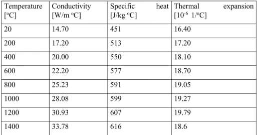
The following properties are modelled as a function of temperature; thermal conductivity, specific heat capacity, density, latent heat and thermal expansion coefficient. The thermal material properties used in the calculations for austenitic stainless steels are based upon data pub-lished by the NRC for 316L [11,12,13,14]. The thermal properties used are summarized in Table 2.

Table 2: Thermal and physical properties as a function of temperature for

stainless steel.

3.2.2 Welding parameters

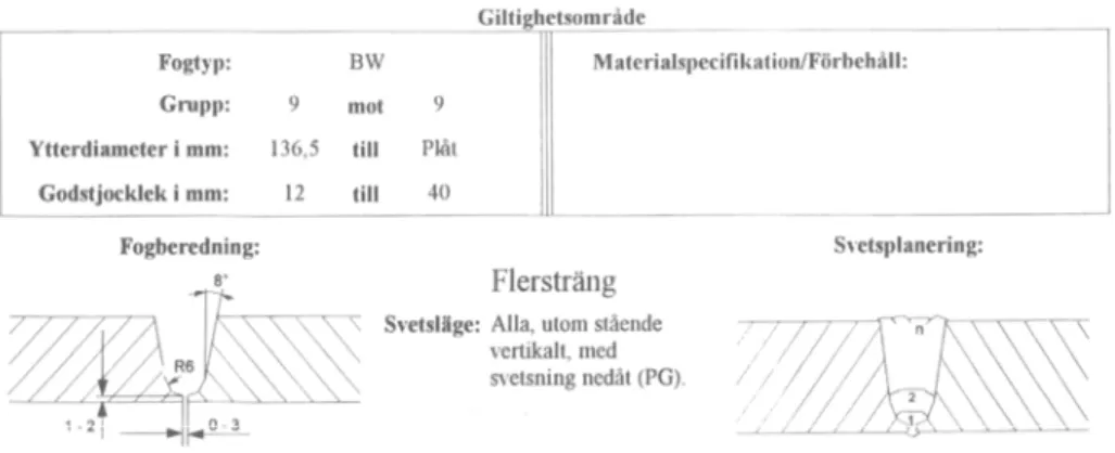
The heat input applied for each weld pass in the analyses is based on parameters from typical welding procedure specifications. Stainless steel butt welds in the Swedish power plants have been welded by both MMA and TIG processes, but probably more frequently by MMA. The root pass is usually TIG. Examples of WPS for stainless steel pipes used in Swedish power plants are shown in Figure 3a and

Temperature

[o_C] Conductivity _[W/mo_C] _[J/kgSpecific o_C] heat Thermal _[10-6 _1/o_C] expansion

20 14.70 451 16.40 200 17.20 513 17.20 400 20.00 550 18.10 600 22.20 577 18.70 800 25.23 591 19.05 1000 28.08 599 19.27 1200 30.93 607 19.79 1400 33.78 616 18.6

(16)

Figure 3a: Example of WPS data (in Swedish) for MMA (SMAW, 111) in

(17)

Figure 3b: Example of WPS data (in Swedish) for TIG (GTAW, 141) in

(18)

3.3 Thermo-plastic mechanical analysis

Stresses and strains generated during the welding are calculated by thermo-mechanical analysis based on the temperature history generat-ed by the procgenerat-edure describgenerat-ed in section 3.2. Large strain theory is applied. Elastic-plastic analysis follows the temperature history on a pass per pass basis, until all weld beads are simulated.

The heating and cooling cycles during multi-pass welding induce cycles of large plastic deformation under temperature variations be-tween room temperature and melt temperature. Modelling of the con-stitutive response under both cyclic plastic straining and for small strain cycles during large temperature variations is a central part for prediction of residual stresses in multi-pass welding.

Incremental plasticity is used with the von Mises yield criterion and associated flow rule. The material hardening law for the austenitic steel is generally assumed to be mixed hardening, with parameters adapted to the available material test data. The temperature-dependent mechanical properties are defined in section 3.3.1. The stainless steel is austenitic at all temperatures and no phase transformation takes place between melting and room temperatures.

Annealing and strain relaxation arises at high temperatures due to mi-crostructural processes as recrystallization and rapid creep. For the rapid temperature transient during welding the dominating process and amount of annealing and relaxation in different regions is not fully understood. Local stress-strain curves for filler material are presented in [15,16] and the measured local yield strength in as-welded filler material and in HAZ corresponds to about 10% strain hardening of the base material, indicating some strain relaxation as simulations com-monly generate higher residual strains. By utilizing the anneal temper-ature capability it is possible to model a tempertemper-ature above which ac-cumulated plastic strains and hardening are reset. Data for the rate of recrystallization or creep at high temperatures is however rare. It has been argued to use an anneal temperature in the range 900 - 1200 °C [5], depending on the dominating relaxation processes and effective time at high temperature. Generally the assumption of a higher anneal-ing temperature results in more conservative results (higher hardenanneal-ing and stresses). Here an annealing temperature of 1000 °C is applied. This modelling approach for strain relaxation at high temperatures or in re-molten material is judged to be sufficiently accurate in relation to uncertainties in other parts of the modeling and available information. Boundary conditions resembling the fixing conditions during the welding are applied to the model. Any post-weld heat treatment and other mechanical loading that may redistribute the residual stress field are modelled, see section 3.1.

(19)

3.3.1 Mechanical material properties

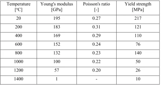
The temperature dependent mechanical material properties are speci-fied based upon data from references [11,12,14,17,18]. Mixed iso-tropic-kinematic hardening models are specified, following recom-mendations in [5,6,9,10]. Based on review of relevant cyclic testing data, the amount of isotropic hardening were limited at high plastic strains by a cut-off which is temperature dependent [6].

The mechanical properties used are summarized in Table 3. For aus-tenitic steel the material hardening is initially rapid from the yield strength [6]. In order to achieve realistic estimates of the residual stresses, it is important to use best-estimates of typical values for the yield properties. Minimum required values for yield strength accord-ing to standards cannot be used, since that result in non-conservative stress.

The mechanical properties used for a filler material in a weld analysis should ideally be measured for just-solidified material, since the work hardening process is included in the weld modeling process itself [5]. Use of as-welded yield data for the filler material would over-predict the residual stresses, since the material then starts from a hardened condition. More relevant data may be measured for filler material in relieved and annealed state or from material deposited by a single-pass to minimize cyclic hardening. For the current filler material it is judged to be a good approximation to apply the same data for the base material and the filler material in initial state. See further discussion on weld strength matching in section 4.4.

Note that the material shows an increase in yield strength with tem-perature above 700 °C. This is due to diffusion and formation of in-termetallic phases at higher temperatures, and consequently interac-tion of plasticity with solutes, called dynamic strain ageing [17].

Table 3: Mechanical properties as function of temperature for stainless steel 316L.

Temperature

[o_C] Young's modulus _[GPa] Poisson's ratio _[-] Yield strength _[MPa]

20 195 0.27 217 200 183 0.31 121 400 169 0.29 110 600 152 0.24 76 800 132 0.23 140

(20)

4 Sensitivity studies

4.1 Sensitivity study for hardening model

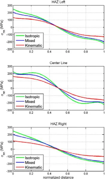
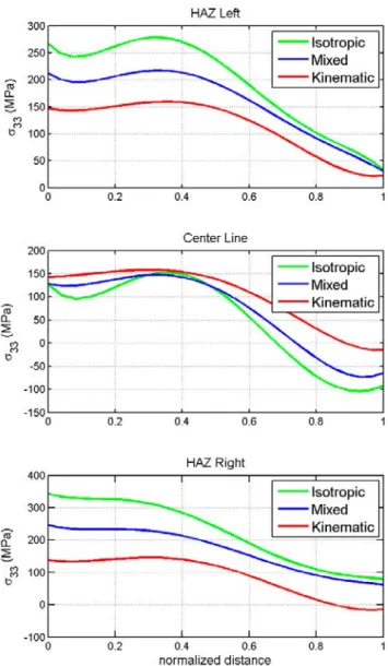
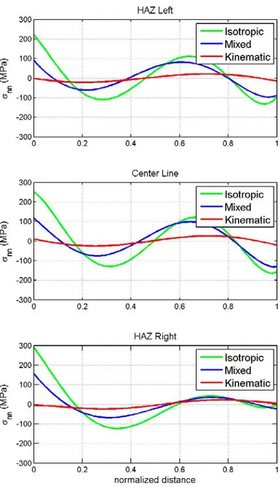
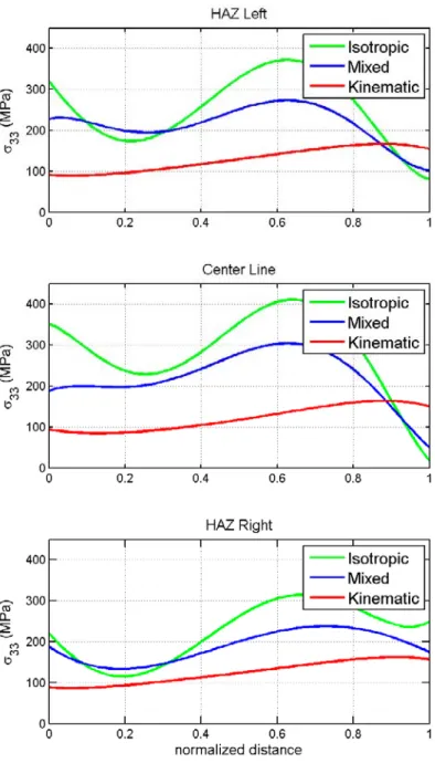
The influence of the hardening model was investigated by applying purely isotropic, purely kinematic and mixed hardening models. See also [6]. The results presented are for stainless steel 316 whose typical room temperature yield strength is 217 MPa. Results are presented in Figure 4a-b and Figure 5a-b for the case of 6 mm and 15 mm thick pipe respectively. Distributions for the axial and hoop stress at 286 °C are presented. Results are presented for paths through the thickness; along the center line of the weld, and along paths in the heat affected zone outside the fusion line, see Figure 13. The results illustrate that isotropic hardening data results in the highest stress amplitudes, kine-matic hardening in substantially lower stresses, and mixed hardening results in levels in between.

Figure 4a: Axial stress at 286 °C along the Center Line and both HAZ of the

(21)

Figure 4b: Hoop stress at 286 °C along the Center Line and both HAZ of the

(22)

Figure 5a: Axial stress at 286 °C along the Center Line and both HAZ of the

(23)

Figure 5b: Hoop stress at 286 °C along the Center Line and both HAZ of the

(24)

4.2 Sensitivity study for pipe radius and bead

size

The influence of the geometry was investigated for all analyzed weld geometries by varying the inner radius of the pipe and bead size. An example of results is presented in Figure 6a-b and 7a-b for a 15 mm thick pipe with R/t = 5 and 10, and for a 65 mm thick pipe with R/t = 3 and 10. The figures show axial and hoop stresses at 286 °C. For these cases the effect of R/t is small for axial stress but significant for hoop stress.

(a)

(b)

Figure 6: Axial stress (a) and hoop stress (b) for 15 mm thick pipe and for

(25)

(a)

(b)

Figure 7: Axial stress (a) and hoop stress (b) for 65 mm thick pipe and for

different pipe geometries; R/t= 3 and 10. (Path at center line, 286 °C)

The influence of the bead geometry was also investigated for all cases. The shape of the cross section of the beads (height to width ratio) was approximated as constant. The bead size may then be described by the dimensionless ratio a/t, where a is the bead height and t the pipe thickness. An example of results when varying bead size is presented by Figure 8 for a 15 mm thick pipe and R/t = 10. Results are shown for the center line path for 286 °C (OT) and 20 °C (RT).

Figure 8a show results for bead size a/t = 0.19 and Figure 8b a/t = 0.28. For this case the effect of a/t is large for the axial stress and more moderate for the hoop stress. For the larger bead size the stress distribution show a change from a sinus like profile towards a more linear profile. The thickness 15 mm is in the thickness range where the stress profile is sensitive, however the smaller bead size is considered more representative.

(26)

Figure 8a: Axial stress σnn and hoop stress σ33 for 15 mm thick pipe for bead

size a/t= 0.19. (R/t = 10, center line path)

Figure 8b: Axial stress σnn and hoop stress σ33 for 15 mm thick pipe for

bead size a/t= 0.28. (R/t = 10, center line path)

The combined influence of pipe geometry and weld bead size on the through thickness profile for the axial stress is illustrated in Figure 9. The pipe geometry is described by the normalized inner radius R/t, and the bead size is described by the dimensionless ratio a/t. That heat input is related to bead size; small beads correspond to low heat input while large beads correspond to high heat input.

(27)

Figure 9 illustrate a transition between linear and sinus-like stress dis-tributions as a function of R/t and a/t. Larger beads and larger inner radius results in a more linear stress distribution, whereas smaller beads and smaller inner radius tends to result in a sinus-like profiles.

Figure 9: Sketch of regions for linear and sinus-like stress distribution for

axial stress as a function of pipe geometry (R/t) and bead size (a/t). transition region

Region of sinus-like axial stress distributions

10 5 a/t R/t 1 Region of linear axial stress distributions

(28)

4.3 Sensitivity study for heat input

The heat input during welding may vary as a result of choice of pa-rameters within the welding procedure. Variations during manufactur-ing also result from for example weldmanufactur-ing speed variations or different welding positions. The power source regulates the current and the arc energy during welding will be determined by the arc length and weld-ing speed. In this section some results are presented from sensitivity studies on influence of heat input on the profile for residual stresses. The profile through the thickness for the axial stress has a general ten-dency to be linear in thin walled pipes and to be of sinus like shape for thick walled pipes. For a certain thickness range there is a transition between these two types of profiles, here the range 10 – 20 mm (me-dium thick pipes). Variations in heat input may especially influence this change in stress profile. Further, a thicker pipe allows heat to dis-sipate quicker into the work piece, which may reduce the sensitivity to variations in heat input.

In general results in this report were determined using typical welding parameters determined from averaged values for the process parame-ters in WPS. Sensitivity studies with respect to heat input have been carried out based on ranges specified for current, voltage and speed in typical WPS for stainless steel pipe welding in Swedish NPPs.

Sensitivity analysis was performed for extreme values of heat input, chosen by studying maximum and minimum values for process pa-rameters in WPS, (Pmin=Umin*Imin/vmax and Pmax=Umax*Imax/vmin).

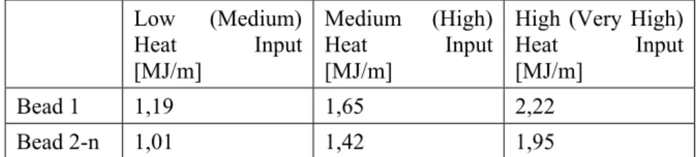
Different WPS for MMA and TIG were studied. Further, welding rec-ords indicated some tendency towards high heat inputs. Sensitivity analyses were performed using the heat input variations in Table 4. Results for the different cases of heat input are labeled by Low, Medi-um and High. Note that for MMA the denotation within parentheses is more appropriate.

Table 4: Variations in heat input applied in sensitivity analyses. (For MMA

the denotation within parentheses is more appropriate.)

Low (Medium) Heat Input [MJ/m] Medium (High) Heat Input [MJ/m]

High (Very High) Heat Input [MJ/m]

Bead 1 1,19 1,65 2,22

Bead 2-n 1,01 1,42 1,95

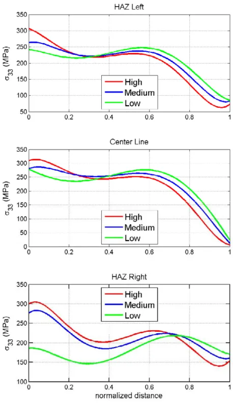
Figure 10 show results from the sensitivity study for a weld in a 12 mm thick pipe with R/t =10. This pipe weld is in the range were the axial stress profile can change from sinus to linear type, and may be sensitive to changes in heat input. Figure 10 show the influence of the heat input on axial and hoop stresses (temperature 286 °C). Stress pro-files are shown along the weld center line and along paths in the heat

(29)

affected zones (to the left and right just outside the weld). It is ob-served that the axial stress along the center line has a more linear stress profile for higher heat input, and a more sinus-like profile for lower heat input. The effect is moderate for the 12 mm pipe. The hoop stress is less sensitive except for the final bead.

(30)

Figure 10b: Hoop stress profiles for different heat inputs (L, M, H) for 12 mm

pipe (R/t=10). Stress profile along the center line and at both HAZ (286 °C).

(31)

4.4 Study of overmatched filler material

Careful selection of weld filler material helps to ensure an as-welded joint with corrosion resistance and mechanical properties that are suit-able for the intended use. The filler may be matched to the base mate-rial regarding corrosion as well as tensile strength.

Consider first matching of filler material for corrosion resistance. Fusion welding results in microstructural segregation which has a det-rimental effect on corrosion resistance. Welds made with matching composition filler material will have less corrosion resistance than the base material. Corrosion resistance equal to or better than the base material can be achieved for the as-welded metal, if filler material with over-matched composition is selected. In an application where a high level of corrosion resistance is required, substantial alloying is needed (Ni, Cr, Mo) [19]. For stainless steel welds in reactor water environment it is usually considered sufficient with slightly higher alloy content, which provide over-matched filler material with respect to corrosion.

Next consider filler material matching with respect to tensile strength. Design codes normally presume the welded joint to be at least as strong as the adjoining base metal. Thus, matching of filler material with respect to mechanical properties are commonly performed with the aim to obtain a tensile strength of the deposited weld that is the same or greater than that of the base material [20]. Generally it is not possible to match both yield strength and tensile strength, and the fo-cus is to match tensile strength. There is no strict definition of strength matching, but if the tensile strength of the as-welded material is within

±70 MPa (i.e. ±10 ksi) from the base material, then the weld common-ly is considered as matching, and otherwise overmatched or under matched with respect to strength. A substantially overmatched weld can influence the collapse behavior, provided that the flow lines are contained within the weld material.

When welding stainless steel the filler metal is usually selected with slightly higher alloy content, and is thus overmatched with respect to corrosion resistance. Strength matching of stainless steel welds in Swedish NPPs can be exemplified by studying the filler Avesta 316L/SKR and the base material 316 L. Typical values for the tensile strength of the base material 316L and of the as-welded Avesta 316L/SKR are 590 MPa for both materials, and the weld is well matched with respect to tensile strength. Typical values for the yield strength 0.2% is 217 MPa for the 316L base material and 460 MPa (as-welded) for Avesta 316L/SKR [21]. The ratios between the tensile

(32)

As discussed in section 3.3.1, the numerical modeling of welding sim-ulates the thermal transients and corresponding large strain cycles that the material is subjected to during welding. The strain history and the corresponding hardening are modelled during the simulation. Filler material that has just solidified should have material properties with-out prior hardening. Stress-strain response measured for just-solidified weld material is not available. For the current stainless steels it is judged to be a good approximation to apply the base material data for the filler material in the initial state.

The large strain cycles during welding will induce substantial harden-ing in the stainless steel weld material, and the yield strength will be much higher for the material in the as-welded state. If yield data measured for as-welded material were used, this could result in over-predicted residual stresses, since the material then would start from an already hardened condition.

We perceive that the filler materials used for stainless steel piping in Swedish NPPs typically have a slightly higher alloy content (for cor-rosion resistance), but we do not expect that the tensile strength has been overmatched. However, it is informative to study the effect of using significantly strength overmatched filler material for stainless steel welds.

The effect of strength overmatched filler material is studied by assum-ing a filler material havassum-ing twice as high yield strength values at all plastic strains and at all temperatures. Figures 11a and 11b present the results for a 20 mm thick pipe (R/t=10) and residual stresses are com-pared for matched and overmatched filler.

Figure 11a shows that the effect of overmatched filler material is small on the axial stress profiles, both at the weld center line and in HAZ. As noted in [2] the axial stresses seem to be mainly governed by the yield properties of the base material.

Figure 11b shows that the effect on the hoop stress profiles. The effect is small in HAZ but significant at the weld center line. The stress level at the center line seems to scale reasonably well with the yield strength of the overmatched filler. The effective plastic strain in the weld is about half for the overmatched filler case compared to the matched filler, but the hardening corresponds to a higher yield strength.

Note that the stress profile for the axial stress in HAZ is most im-portant for stainless steel piping, since this is the position were stress corrosion cracking could occur and result in long cracks along the HAZ of the weld.

(33)

Figure 11a: Comparison of axial stress profiles for matched and

over-matched filler material for 20 mm thick pipe (R/t=10). Stress profiles along the weld center line and along HAZ Left (20 °C).

(34)

Figure 11b: Comparison of hoop stress profiles for matched and

over-matched filler material for 20 mm thick pipe (R/t=10). Stress profiles along the weld center line and along HAZ Left (20 °C).

(35)

5 Comparison to experimental results

Comparison to experimental measurement of residual stress profiles in different stainless steel pipe welds is presented in the development reports [5] and [6] that were made before this work. Comparison was made for three different cases of butt-welded stainless steel pipes with thickness 15.9 mm (R/t=25), 19 mm (R/t=10.5) and 65 mm (R/t=3). Figure 12 shows comparison of the numerical results to DHD meas-urements for a 65 mm thick pipe and R/t =3 [22]. The axial and hoop stress distributions along the center line of the weld are shown at 20 °C. The results show good agreement for the axial stress and mod-erate agreement for the hoop stress. The agreement for the hoop stress is improved when analyzing the exact pipe geometry, see [5].

Figure 12: Comparison between measured and numerically determined

residual stresses for 65 mm thick stainless steel pipe butt-weld. Axial and hoop stresses along the center line (20 °C).

Cases for comparisons were collected in [5], but there exist few new published results for measured residual stresses in stainless steel pipe welds and cases found are for various geometries. For validation it would have been very valuable with measurements performed for a series of cases where the pipe geometry is systematically varied, and possibly also various cases of heat input for thicknesses in the region for transition of stress profile. In addition the methods for

(36)

measure-6 Results for recommended residual

stress profiles

6.1 Overview of cases and basis

Results are presented for butt-welds between stainless steel pipes of different thickness. The weld and pipe geometry is principally the same for all cases as illustrated in Figure 13. Parameters describing the series of cases defining the recommended stress profiles are sum-marized in Table 4. Results are presented for three different paths through the thickness; along the center line of the weld, and along paths in the heat affected zone (just outside the fusion line). The ar-rows in red color represent the different paths; HAZ Left, Center Line and HAZ Right. The coordinate is zero at the pipe inside.

Figure 13: General weld geometry and results paths.

Table 4: Parameters defining cases for stainless steel pipe butt-welds.

Thickness t [mm]

Pipe radius to thickness ratio

Rin/t

Material Welding _process Heat input, first bead [MJ/m] Heat input, other beads [MJ/m] Number of passes 6 10 316L TIG/MMA 1.65 0.94 5 10 10 316L TIG/MMA 1.65 1.1 11 12 10 316L TIG/MMA 1.65 1.42 19 15 10 316L TIG/MMA 1.65 1.42 23 20 10 316L TIG/MMA 1.65 1.55 31 25 10 316L TIG/MMA 2.3 1.71 26 65 10 316L TIG/MMA 2.3 1.71 104

Below is a discussion of the assumptions and parameter values used in the analysis of cases for the development of recommended residual stress profiles.

The series of pipe geometries selected for analysis will cover most piping in the NPPs. The selected thicknesses should capture the change in stress profile for pipe thicknesses in the range 10 – 20 mm. Stainless steel pipes in the plants typically have a pipe radius to thick-ness ratio (R/t) in the range 7 to 15. The ratio R/t =10 is considered

Center Line

HAZ Right HAZ Left

(37)

representative and high enough to produce conservative results with respect to the axial residual stress at the pipe inside (considering SCC from the inside).

Axisymmetric modelling is used and variation for the through thick-ness stress profile at different positions around the circumference is assumed to be small. The assumption is judged acceptable for welding processes where start/stop positions occur at random positions around the circumference, and not at the same position for all beads. Thinner wall thicknesses can be expected to imply larger variation.

The distance between the weld and any other weld or larger disturb-ance (rapid change in wall thickness) is assumed to be larger than 2.5√��. If this condition is not fulfilled, then the influence of the oth-er weld or disturbance need to be analyzed.

The base cases are developed for stainless steel 316L material behav-ior, with a typical yield strength of 217 MPa at room temperature. (The minimum required yield strength according to ASME is 170 MPa for 316L.) Mixed hardening is applied using data as described in section 3.3.1.

Some sensitivity analyses were performed to assess the effect of stain-less steels with different yield and hardening properties. Cases corre-sponding to initial yield strengths of 150 MPa and 325 MPa were ana-lyzed. The assumption that the filler material is, as customary, matched to the base material is included, and both materials have the same initial properties. Similar stress profiles were obtained and these analyses suggest that scaling by the typical yield strength can be used to account for moderate differences in yield properties for stainless steels. Scaling of the results presented in the report is assessed to be valid for stainless steels with typical yield strength in the range 150 MPa to 325 MPa.

The residual stress results presented in this report are for 316L. For assessment of other stainless steels all stress components can be scaled by the typical yield strength of 217 MPa at room temperature.

The heat inputs used are indicated in Table 4, and are determined from process parameters in typical WPS for stainless steel pipe welding in Swedish NPPs. The applied heat inputs are medium if the welding were TIG, and slightly higher than medium if MMA welding (which is conservative with respect to axial stress at the pipe inside). See also discussion in section 4.3. The height to width ratio of the weld beads

(38)

with design pressure 8.6 MPa. The test pressure is about 22 MPa for pressurized water reactors (PWR) with design pressure 17.1 MPa. The lower test pressure was applied in order for the results to be conserva-tive and applicable to all reactors. The redistribution of the axial stress due to the pressure test was very small, provided that the distance is > 2.5√�� to larger disturbances (rapid change in wall thickness). The reduction of the hoop stress due to the pressure test is small at the in-ner part of the pipe wall, but substantial (about 100 MPa) at the outer part of the pipe wall, see Fig B9 – B11 in Appendix B.

6.2 Definition of recommended stress profiles

The recommended residual stress profiles are based on analyses using typical values for the influencing parameters as described in sec-tion 6.1.A range of sensitivity analyzes were performed. For cases sensitive to realistic variations from typical values, the selected results are conservative with respect to the inner part of the pipe (SCC growth from the inside).

The weld residual stress profiles are described by polynomials for paths at the weld center line and in HAZ, as described in Figure 13. The weld beads are added one after another, which makes the stress distribution different for the HAZ at each side of the weld (even if the joint geometry is symmetrical). Results are given only for the most conservative HAZ path. Results are given for axial stress, ��

(trans-versal stress, perpendicular to the direction of the weld), and for hoop stress, �� (longitudinal stress, in the direction of the weld).

The residual stress profiles are normalized with the amplitude parame-terSr, which is defined as the typical yield strength of the base

mate-rial at room temperature. This normalization allows estimation for different stainless steels by adjustment for the difference in yield properties. Note that the definition of Sris different from previous

recommendations [1].

In fact Srcould be the typical 0.2% offset yield strength of the

un-hardened filler material. However, for these stainless steel joints with strength matched filler material, it is considered to be a good approx-imation to apply the base material data for the filler material in its ini-tial unhardened state.

It is customary to use strength matched filler material and this is as-sumed in the calculations. In a case of overmatched filler material, the hoop stress at the center line of the weld need to be scaled separately, as discussed in section 4.4. Specific analyses can be recommended for significantly over or under matched filler material.

(39)

In order to obtain realistic estimates of the weld residual stresses, the typical (or best estimate) yield strength shall be used, and not the min-imum required. In general, typical yield strength of stainless steel may be estimated from minimum required values by using a factor of 1.35. The temperature dependence of the residual stress field is described through a coefficient CT entering the hoop stress polynomial. Note that

this again differs from previous recommendations in [1].

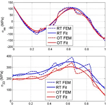
The recommended through-thickness weld residual stress profiles are described by 5th_{order polynomials of the form}

� ��_{�� }� �� _�� _�� _�� _�� _�� where �� is the normalized position along the path and �� are

coeffi-cients. The coefficients are presented in section 6.3 – 6.9 for different wall thicknesses. For thicknesses between the available cases, linear interpolation is recommended. Linear interpolation of the coefficients for two surrounding thicknesses may be applied for establishment of stress profiles for intermediate geometries. Extrapolation for thick-nesses below 6 mm or above 65 mm must be performed with caution. Detailed results for the residual stress field are given in Appendix A for the different thicknesses. In the appendix the denotation RT is used for room temperature and OT is used for the operation temperature 286°C (BWR). The influence of temperature is small and other tem-peratures are assessed by the relations given in section 6.3 – 6.9. Welds deviating substantially from the conditions assumed in the analyses of the base cases need to be handled with specific simula-tions and assessments. Causes may include; large difference in weld joint geometry, deviation from pipe geometry, R/t below 7, rapid change in thickness or other weld closer than 2.5√��. An important case is final installation weld with high restraints (system closure weld). Other causes could be welding performed with constant start/stop positions or possibly 3D effects for very thin walled pipes. An overview of the stress profiles is presented in Figure 14 with re-sults along the weld center line path at 286 °C for axial and hoop stress.

(40)

Figure 14a. Axial residual stress in pipe butt weld along the weld centerline at 286 °C.

(41)

6.3 Thickness 6 mm

The weld residual stresses across the pipe wall are described by a 5th

degree polynomial. The coefficients in Table 5 and Table 6 enter the polynomial below, values are in MPa:

��= �� _�� _�� _�� _�� _�� ] ��= �� _�� _�� _�� _�� _�� ] �� = −_{5320 � �}3 269₂₆₆

Note that only the hoop stress �� is temperature dependent. The

coef-ficient �� is 1.0 at 20°C, 0.85 at 286°C (BWR) and 0.82 at 345°C

(PWR).

Table 5: Coefficients for polynomial fit. Hoop stress along paths.

Position c0 c1 c2 c3 c4 c5

Center Line 0.63983 -0.5842 5.3703 -8.4527 -1.4992 4.3204 HAZ 0.68005 -2.646 24.875 -72.381 82.68 -33.282

Table 6: Coefficients for polynomial fit. Normal stress along paths.

Center Line 1.08 -2.4157 16.907 -58.2 64.605 -23.274 HAZ 0.82083 -0.9928 8.7745 -35.06 36.715 -10.9

(42)

6.4 Thickness 10 mm

The weld residual stresses across the thickness are fitted by a 5th

de-gree polynomial. The coefficients in Table 7 and Table 8 enter the polynomial below, values are in MPa:

��= �� _�� _�� _�� _�� _�� ] ��= �� _�� _�� _�� _�� _�� ] �� = −_{5320 � �}3 269₂₆₆

(PWR).

Center Line 1.6752 0.93035 -23.766 81.924 -104.33 43.827 HAZ 1.7078 -3.9284 5.5123 15.199 -40.257 22.265

Center Line 0.45756 -0.0517 -2.3712 9.0886 -16.37 8.2058 HAZ 0.70596 -0.0721 -22.177 74.102 -89.242 36.213

(43)

6.5 Thickness 12 mm

��= �� _�� _�� _�� _�� _�� ] ��= �� _�� _�� _�� _�� _�� ] �� = −_{5320 � �}3 269₂₆₆

(PWR).

Center Line 1.4974 1.3405 -17.974 58.279 -71.413 28.589 HAZ 1.4571 1.9368 -29.033 87.281 -98.721 37.997

Center Line 0.17729 -0.8621 1.6547 9.6666 -23.651 12.109 HAZ 0.55671 -2.3266 -6.9121 38.515 -51.099 20.941

(44)

6.6 Thickness 15 mm

��= �� _�� _�� _�� _�� _�� ] ��= �� _�� _�� _�� _�� _�� ] �� = −_{5320 � �}3 269₂₆₆

(PWR).

Center Line 1.0065 2.3163 -19.086 66.405 -84.172 34.034 HAZ 1.2199 1.3998 -21.2 76.455 -97.268 40.05

Center Line 0.55005 -5.6076 -6.0824 81.908 -128.89 57.506 HAZ 0.71522 -7.0415 8.5096 20.509 -41.481 18.754

(45)

6.7 Thickness 20 mm

��= �� _�� _�� _�� _�� _�� ] ��= �� _�� _�� _�� _�� _�� ] �� = −_{5320 � �}3 269₂₆₆

(PWR).

Center Line 0.77832 -5.2064 29.019 -40.918 22.702 -5.3028 HAZ 0.68776 -3.3748 14.179 -4.1386 -13.024 6.4001

Center Line 1.0159 -8.5275 -16.027 117.77 -155.8 61.818 HAZ 1.1901 -13.026 14.346 46.243 -93.157 45.571

(46)

6.8 Thickness 25 mm

��= �� _�� _�� _�� _�� _�� ] ��= �� _�� _�� _�� _�� _�� ] �� = −_{5320 � �}3 269₂₆₆

(PWR).

Center Line 0.54484 -3.1805 13.704 4.8588 -30.401 15.26 HAZ 0.5826 -6.3136 28.166 -26.957 -0.3649 6.1033

Center Line 1.0336 -10.661 -13.038 130.6 -179.36 71.16 HAZ 1.1723 -16.715 36.009 2.5435 -51.381 28.837

(47)

6.9 Thickness 65 mm

��= �� _�� _�� _�� _�� _�� ] ��= �� _�� _�� _�� _�� _�� ] �� = −_{5320 � �}3 269₂₆₆

(PWR).

CenterLine 0.30363 1.4197 30.508 -127.86 187.51 -91.346 HAZ 0.40251 -1.5626 35.586 -110.16 136.47 -59.788

CenterLine 1.1503 -25.678 135.25 -335.57 391.81 -167.22 HAZ 0.8861 -17.565 72.584 -143.05 144.71 -56.978

(48)

7 Differences to previous

recom-mended stresses

New recommendations for stress distributions have been developed for butt welds in stainless steel pipes. Below the earlier recommended stress profiles are described and discussed in relation to the new rec-ommended stress profiles.

The earlier recommendations for residual stresses were based on anal-yses performed 1996 [2] which used the best knowledge at that time. Since then developments within measurement methods and calcula-tion of residual stresses has indicated a need to update the earlier rec-ommendations. Recent development and validation projects have re-sulted in changes, including deviation from assumption of kinematic hardening, yield data from measurements for as-welded material, and use of upper bound heat input.

The earlier recommended stress profiles for stainless steel pipes are presented in Figures 15a-b. The hoop stress σ33 is constant regardless

of the thickness. The axial stress σnn is linear for thicknesses below

30 mm and shows a sinus-like shape for thicknesses over 30 mm. The slope of the linear axial stresses decreases with increasing thickness. In addition the amplitudes differ; Sr was 348 MPa and 187 MPa for the weld and the base material respectively.

Figure 15a: Earlier recommendation for hoop stress along center line and HAZ.

(49)

Figure 15b: Earlier recommended axial stress along center line and HAZ.

From Figures 14a-b and 15a-b the new and previous recommended stresses can be compared. The main difference is the change in stress profile shapes, with a stronger trend for sinus type profiles. In earlier results, only axial stress over a 30 mm thickness showed a sinus like distribution. All other stresses were either constant or linear. The pre-sent results show a transition between linear to sinus type distribution for thicknesses around 12 mm to 15 mm for the axial stress. The new recommended weld residual stresses are based on new knowledge developed within numerical welding simulation. In addi-tion efforts have been made to reduce conservatism by using typical data for influencing parameters. Since upper bound crack growth rela-tions are applied when analyzing stress corrosion cracking, it would be very conservative to apply also upper bound assumptions for the residual stresses. For this reason realistic values have been sought for regarding the influencing parameters.

As for all types of loads, new weld residual stresses should be consid-ered and assessments updated when significant new knowledge exist. The new recommended stress profiles presented in section 6 can result in slower crack growth for many cases, but in some cases also faster crack growth.

Note that when more realistic residual stress profiles are used, (and not conservative upper bound profiles), it is increasingly important to perform sensitivity studies as part of defect tolerance assessments.

(50)

8 Conclusions

Residual stresses in stainless steel pipe butt-welds have been analyzed by numerical weld simulation, with the purpose to develop recom-mended residual stress profiles to apply in damage tolerance analyzes. Recent progress in measurement methods and in simulation of weld residual stress has shown a need for establishment of new recom-mended residual stress profiles. Development of heat source model-ling and material modelmodel-ling for welding simulation has been per-formed, together with validation to measurements [5,6,10]. These pre-ceding projects provide the basis for the numerical analyses of differ-ent cases performed in this report.

Recommended through-thickness weld residual stress distributions have been developed. Detailed numerical welding simulations have been performed for a set of cases covering most stainless steel piping in Swedish NPPs, together with sensitivity studies with respect to ma-terial modelling, pipe geometry and heat input. Best-estimate typical data have been used for influencing parameters with the aim to estab-lish realistic through-thickness stress distributions to be applied in integrity assessments, especially for stress corrosion crack growth. Recommended residual stresses are presented along paths in the cen-ter line of the weld and in the heat affected zones. In section 6 of the report the recommended stress profiles are given as polynomials for each analyzed weld case. For intermediate geometries it is mended to apply linear interpolation. Compared to earlier recom-mendations the axial residual stress profiles generally show a strong-er trend for sinus type distributions.

Welds deviating from the conditions assumed in the analyses of the base cases are recommended to be handled with specific simulations. Examples that may lead to significant deviation include; deviation from pipe geometry, R/t below 7, rapid change in thickness or other weld closer than 2.5√Rt, or large difference in weld joint geometry. An important case is final installation weld with high restraints (sys-tem closure weld). Other causes could be welding performed with constant start/stop positions or 3D effects for very thin walled pipes.

(51)

9 References

[1] Dillström P, Bergman M, Brickstad B, et al., "A combined de-terministic and probabilistic procedure for safety assessment of components with cracks - Handbook," Swedish Radiation Safety Authority, SSM 2008:01, 2008.

[2] B. Brickstad and L. Josefson, "A Parametric Study of Residual Stresses in Multipass Butt-Welded Stainless Steel Pipes," SAQ FoU-Report 96/01,.

[3] P. Delfin, B. Brickstad, and L. Josefson, "Residual Stresses in Multi-Pass Butt-Welded Bimetallic Piping, Part I," SAQ FoU-Report 98/12,.

[4] P. Delfin, B. Brickstad, and J. Gunnars, "Residual Stresses in Multi-Pass Butt-Welded Bimetallic Piping, Part II," SAQ FoU-Report 99/06,.

[5] W. Zang, J. Gunnars, P. Dong, and J.K. Hong, "Improvement and validation of weld residual stress modelling procedure, SSM re-search report 2009:15," ISSN-2000-0456, 2009.

[6] J. Mullins and J. Gunnars, "Influence of Hardening Model on Weld Residual Stress Distribution," SSM Report 2009:16, 2009. [7] M.C. Smith and Smith A.C., "NeT bead-on-plate round robin:

Comparison of residual stress prediction and measurements," Int J Presuure Vessels and Piping, Vol 86, pp 79-95, 2009.

[8] J. Mullins and J. Gunnars, "Deformation Histories Relevant to Multipass Girth Welds: Temperature, Stress and Plastic Strain Histories," Mat. Sci. Forum, Vol. 681, pp. 61-66, 2010.

[9] J. Mullins and J. Gunnars, "Welding simulation - Relationship between welding geometry and determination of hardening mod-el," PVP2012-78599, 2012.

[10] J. Mullins and J. Gunnars, "Validation of Weld Residual Stress Modeling in the NRC International Round Robin," Swedish Ra-diation Safety Authority, SSM Report 2013:01.

[11] US NRC, "International Weld Residual Stress Round Robin Problem Statement, Version 1," Office of Nuclear Regulatory Research - Component Integrity Branch, 2009.

[12] US NRC, "The Battelle Integrity of Nuclear Piping (BINP) Pro-gram Final Report," NUREG/CR-6837 Vol. 2, 2005.

[13] "Review and Analysis of the Davis-Besse March 2002 Reactor Pressure Vessel Head Wastage Event, Appendix A - Finite Ele-ment Stress Analysis of Davis-Besse CRDM Nozzle 3 Penetra-tion," ML070860281, NRC, 2007.

(52)

Mechanics and Materials, vol. 7-8, pp. 127-132, 2007.

[16] Edwards, L., et al., "Advances in Residual Stress Modeling and Measurement for the Structural Integrity Assessment of Welded Thermal Power Plant," Advanced Materials Research, vol. 41-42, pp. 391-400, 2008.

[17] L. Lindgren, K. Domkin, and S. Hansson, "Dislocations, vacan-cies and solute diffusion in physical based plasticity model for AISI 316L," Mechanics of Materials, Vol 40, pp. 907-919, 2008. [18] Hong, S-G, et al, "Temperature effect on the low-cycle fatigue

behavior of type 316L stainless steel: cyclic non-stabilization and an invariable fatigue parameter," Mat Sci Eng A, Vol 457, pp139-147, 2007.

[19] Crum, J. R., et. al., "Special Alloys and Over-matching Welding Products Solve FGD Corrosion Problems," Technical Paper, Spe-cial Metals Welding Products, NACE Conf. 1996.

[20] R. S. Funderburk, "Selecting Filler Metals: Matching Strength Criteria," Welding Innovation Vol. XVI, No. 2, 1999.

[21] "Filler Metals for Joining Applications," Product brochure, p. 110 Avesta 316L/SKR, www.boehler-welding.com/Downloads, voestalpine Böhler Welding, 2015.

[22] Bate, S.K., et al., "Measurement and Modelling of Residual Stress in Thick Section Type 316 Stainless Steel Welds," Proc. 6th Int. Conf. on Residual Stresses, ICRS6, pp.1511-1518, 2000.

(53)

10 Appendix A – Detailed results

10.1 Weld thickness 6 mm

Figure A1: Hoop stress (S33) at: (a) Room Temperature (RT) and (b) Opera-tion Temperature (OT) for weld thickness 6 mm.

Figure A2: Axial stress (S22) at: (a) Room Temperature (RT) and (b) Opera-tion Temperature (OT) for weld thickness 6 mm..

(a) (b) (a) (b)

(54)

Figure: A3: (a) Hoop stress S33 and (b) Axial stress S22 at Operation Tem-perature (OT) for weld thickness 6 mm.

(a) (b)

(55)

(56)

(57)

Figure A6: Hoop and axial stresses at the inner surface at Operating Tem-perature (OT) for weld thickness 6 mm.

(58)

10.2 Weld thickness 10 mm

Figure A7: Hoop stress (S33) at: (a) Room Temperature (RT) and (b) Opera-tion Temperature (OT) for weld thickness 10 mm.

Figure A8: Axial stress (S22) at: (a) Room Temperature (RT) and (b) Opera-tion Temperature (OT) for weld thickness 10 mm.

(a) (b)

(59)

Figure A9: (a) Hoop stress S33 and (b) Axial stress S22 at Operation Tem-perature (OT) for weld thickness 10 mm.

(a) (b)

(60)

(61)

(62)

(63)

10.3 Weld thickness 12 mm

Figure A13: Hoop stress (S33) at: (a) Room Temperature (RT) and (b) Op-eration Temperature (OT) for weld thickness 12 mm.

Figure A14: Axial stress (S22) at: (a) Room Temperature (RT) and (b) Oper-ation Temperature (OT) for weld thickness 12 mm.

(a) (b)

(64)

(a) (b)

(65)

(66)

(67)

(68)

10.4 Weld thickness 15 mm

Figure A20: Axial stress (S22) at: (a) Room Temperature (RT) and (b) Oper-ation Temperature (OT) for weld thickness 15 mm.

(a) (b)

(69)

(a) (b)

(70)

(71)

(72)

(73)

10.5 Weld thickness 20 mm

Figure A26: Axial stress (S22) at: (a) Room Temperature (RT) and (b) Oper-ation Temperature (OT) ) for weld thickness 20 mm.

(a) (b)

(74)

Figure A27: (a) Hoop stress S33 and (b) Axial stress S22 at Operation Tem-perature (OT) ) for weld thickness 20 mm.

(a) (b)

(75)

(76)

(77)

Figure A30: Hoop and axial stresses at the inner surface at Operating Tem-perature (OT) ) for weld thickness 20 mm.

2016:39 Recommended residual stress profiles for stainless steel pipe welds

Research

Recommended residual stress profiles

for stainless steel pipe welds

2016:39

2016:39

Recommended residual stress

Recommended residual stress profiles

for stainless steel pipe welds

Contents

1 Background

2 Scope

3 Modeling

3.1 Manufacturing sequence

3.2 Transient thermal analysis

3.2.1 Thermal material properties

3.2.2 Welding parameters

3.3 Thermo-plastic mechanical analysis

3.3.1 Mechanical material properties

4 Sensitivity studies

4.1 Sensitivity study for hardening model

4.2 Sensitivity study for pipe radius and bead

size

4.3 Sensitivity study for heat input

4.4 Study of overmatched filler material

5 Comparison to experimental results

measure-6 Results for recommended residual

stress profiles

6.1 Overview of cases and basis

6.2 Definition of recommended stress profiles

6.3 Thickness 6 mm

6.4 Thickness 10 mm

6.5 Thickness 12 mm

6.6 Thickness 15 mm

6.7 Thickness 20 mm

6.8 Thickness 25 mm

6.9 Thickness 65 mm

7 Differences to previous

recom-mended stresses

8 Conclusions

9 References

10

Appendix A – Detailed results

10.1

Weld thickness 6 mm

10.2

Weld thickness 10 mm

10.3

Weld thickness 12 mm

10.4

Weld thickness 15 mm

10.5

Weld thickness 20 mm