Inventory Control of Finished Goods
for the Aftermarket
Authors:
Sercan Eminoğlu, LTH Joan Esteve i Magrané, UPC - LTH
(exchange student)
Examiner:
Johan Marklund, LTH
Supervisors:
Peter Berling, LTH
Hannu Kauppinen, TitanX Engine Cooling AB
i
Preface
This master’s thesis presents a degree project performed at TitanX Engine Cooling AB in the department of supply chain. This thesis has been performed by Sercan Eminoglu, a student in the master’s program in Logistics and Supply Chain Management and Joan Esteve i Magrané, an exchange student in master’s program in Industrial Engineering. This thesis has been our last step towards becoming Masters of Science in Industrial Engineering and Management and it has been a wonderful opportunity to put our theoretical knowledge gathered throughout our studies to practice in a real-world situation.
We would like to thank the company TitanX and especially our supervisors Hannu Kauppinen and Niklas Möller for giving us this chance and for guiding us throughout this journey. We would also like to thank our examiner Johan Marklund for his reflections willingness to collaborate with us, and finally we want to show our sincerest appreciation to our supervisor at Lund University, Peter Berling, for his continuous help and dedication towards ensuring the success of this project.
Lund, June 2017
iii
Abstract
Title
Inventory control of finished goods for the aftermarket.
Authors
Sercan Eminoglu Joan Esteve Magrané Supervisors
Peter Berling, Faculty of Engineering, LTH Hannu Kauppinen, TitanX Engine Cooling AB Niklas Möller, TitanX Engine Cooling AB
Background
TitanX Engine Cooling is a global supplier of powertrain cooling solutions to commercial vehicles, both for OEMs and the independent aftermarket. The company with annual sales of over 1.6 billion SEK (US$ 192 million) has some 800 employees worldwide. TitanX is headquartered in Gothenburg, Sweden and has manufacturing sites in Sweden, USA, Brazil, China and Mexico.
Its manufacturing facilities are designed and operated with a strong and continuous application of lean manufacturing principles, and they perceive themselves as a very flexible supplier. The production sites have a high level of vertical integration, including the manufacturing of key critical components to ensure the highest quality results. The production operations are continuously adjusted to meet variations in customer demand. The vision is to be the number one global supplier of powertrain cooling solutions to the commercial vehicle industry.
The facility in Sölvesborg consists of three zones; a raw material warehouse, a shop floor, and a finished goods warehouse. TitanX generally keeps high inventory levels of raw material and finished goods. An important reason for this is the marketing strategy to increase the current market share above 30% of the independent aftermarket for truck engine cooling systems. Therefore, high customer service levels and high efficiency are key performance measures that drive high capacity and stock levels.
iv
Purpose
The purpose of the degree project is to analyze the finished goods inventory for independent aftermarket products to provide both more accurate forecasting methods and a scientific approach for controlling these inventories by finding the reorder points for a given service level and considering trade-offs between the production lead times and the safety stock needed for those.
Methods
Liebermann & Hillier (2001) described all the major phases of a typical operations research (OR) modeling approach used to conduct the research in this project.
Quality assurance was done by a process of validation and verification based on Banks, Carson II, Nelson, and Nicol, (2005)
Data collection was done using semi-structured interviews, direct observation, literature review and data provided by the company.
By using those, a new forecasting model and inventory control tool have been developed and the results have been compared to the older model provided by the company to observe the level of improvement obtained.
Conclusions
New forecasting model improves upon the results of the previous one by 21,2% in terms of forecasting accuracy for a specific available sample.
The implemented inventory control tool is a new advancement that the company previously did not possess and remarkably diminishes the required safety stock levels by 59% which accounts for 279.783,5 €/year.
Finally, the tools provided will save planning time and will allow for the comparison of different scenarios.
Keywords
Aftermarket products, forecasting, operations research, intermittent demand patterns, inventory control.
v
List of abbreviations, variables and parameters
List of variables and parameters
P Average inter-demand interval
CV2 Squared coefficient of variation of the
demand size
squared coefficient of demand size variation
during the lead time
L Lead time
Λ Mean number of arrivals per time unit
N Number of periods with demand
ti Period i=1…T
Σ Standard deviation of the historic demand
data
µ Mean of the historic demand data
Initial value of the mean demand
Mean demand size of the periods where
demand has occurred, only considering the first τ periods
Τ Number of periods used for initialization
Q Time until the next demand during the current
iteration of the forecast iteration
T Last period in the historic data
or Real demand in period t
Expected inter-demand interval in period t
Expected demand size in period t if the
demand is positive
Forecast in units/period
Smoothing constant for p
Smoothing constant for z
Simple Exponential Smoothing forecast in
period t
Α Smoothing constant for Simple Exponential
Smoothing
MAD Mean Absolute Deviation
N Number of periods used in the forecast
S1 Probability of no stock out per order cycle
S2 “fill rate”- Fraction of demand that can be
vi
S3 “ready rate”- Fraction of time with positive
stock on hand
R or s Reorder point
Q Batch size
S Maximum inventory level
Probability of having k customers in one
period
Probability of demand size j
Var Variance
D(t) Demand of period t
P(D(t)=X) Probability of the demand of a period being X
P Success probability in each experiment
R Number of failures until the experiment is
stopped
Mean expected demand during the lead time
Standard deviation of the forecasts during the
lead time
Density function of the Gamma distribution
Cumulative probability distribution of the
Gamma distribution
r (gamma distr.) Parameter from the gamma distribution
Probability distribution function of the
standardized normal distribution
Probability density function of the
standardized normal distribution
Loss function of the normal distribution
F(x) Probability distribution function of demand
size x
RU Upper bound of the reorder point used in the
inventory control iterative process
RL Lower bound of the reorder point used in the
vii
List of abbreviations
E Expected
MAD Mean Absolute Deviation
MSE Mean Squared Error
OEM Original Equipment Manufacturer
OES Original Equipment Supplier
IAM Independent AfterMarket
NBD Negative Binomial Distribution
SBA Syntetos and Boylan Approximation
SKU Stock Keeping Unit
SES Simple Exponential Smoothing
OR Operations Research
L Lead time
MPS Master Production Schedule
ix
Table of contents
Preface i
Abstract iii
List of abbreviations, variables and parameters v
List of tables xi
List of figures xiii
1. Introduction 1 1.1. Background 1 1.2. Problem description 2 1.3. Purpose 4 1.4. Research questions 4 1.5. Research limitations 4 1.6. Contribution to knowledge 4 2. Methodology 5 2.1. Research method 5 2.2. Quality Assurance 9 2.2.1. Validation 9 2.2.2. Verification 9 2.3. Data collection 10 2.3.1. Interview 10 2.3.2. Direct observation 12 2.3.3. Literature review 12
x
2.3.4. Data provided by the company 13
3. Theory 15 3.1. Forecasting 15 3.1.1. Demand patterns 15 3.1.2. Demand segmentation 17 3.1.3 Forecasting methods 19 3.2. Inventory control 22
3.2.1. Different ordering systems 23
3.2.2. Single-echelon systems determining reorder points 24
4. Empirical data 31
4.1. Company overview 31
4.2. System description 31
4.3. Empirical data sets 34
5. Analysis 37
5.1. Forecast 38
5.1.1. Seasonality and trend 38
5.1.2. Demand segmentation 41
5.1.3. Comparing with the previous forecast 45
5.2. Inventory control 48
5.2.1. Inventory control model 48
5.2.2. Comparison to previous model 53
6. Discussion 56
7. Conclusion 60
xi
List of tables
Table 4. 1 - Lead time of products based on ABC categorization. ...36
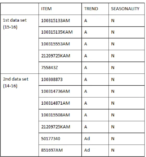
Table 5. 1 - Items with observed seasonality and/or trend patterns. ...41
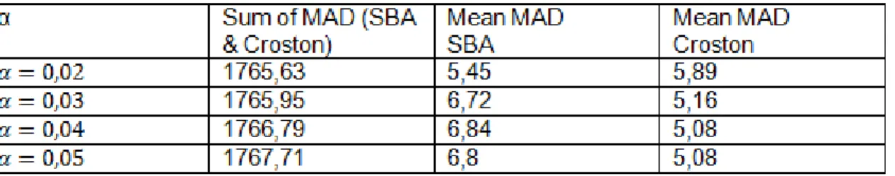
Table 5. 2 - Sensitivity analysis of alpha value for weekly demand. ...43
Table 5. 3 - Number of items categorized in each region. ...44
Table 5. 4 - Sum and mean of errors for weekly and monthly aggregation levels. ...45
Table 5. 5 - Sum of errors and number of optimal items for each forecasting tool. ...46
Table 5. 6 - Upper & lower bounds for different conf. intervals as well as distance to the expected value. ...47
Table 5. 7 - Weekly demand for an artificial item. ...49
Table 5. 8 - Resized weekly demand for an artificial item. ...49
Table 5. 9 - Analysis of reorder points for each service level. ...52
xiii
List of figures
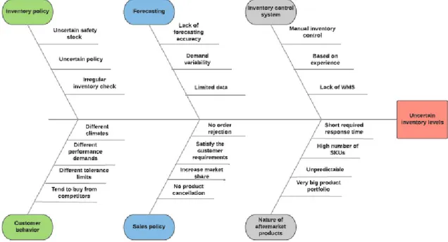
Figure 1. 1 - Cause and effect diagram for IAM products. ... 3
Figure 3. 1 - Graphic representation of different demand patterns...16
Figure 3. 2 - The framework for the implementation of a categorization scheme (Bucher, D., & Meissner, J., 2011). ...18
Figure 3. 3 - Categorization scheme for a single-echelon inventory configuration (Bucher, D., & Meissner, J., 2011). ...25
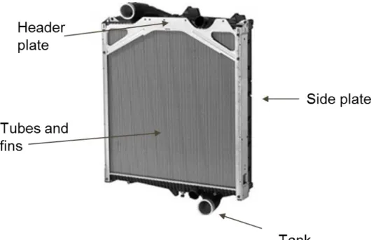
Figure 4. 1 - Engine cooling module. ...32
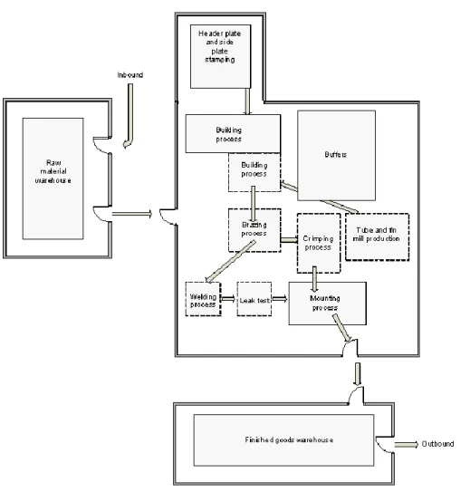
Figure 4. 2 - Internal flow. ...33
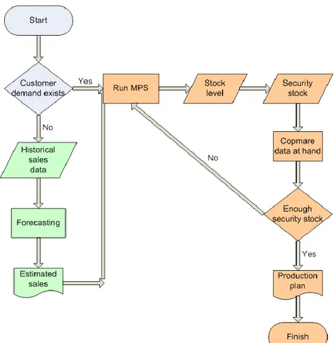
Figure 4. 3 - A flow chart for the MPS procedure. ...34
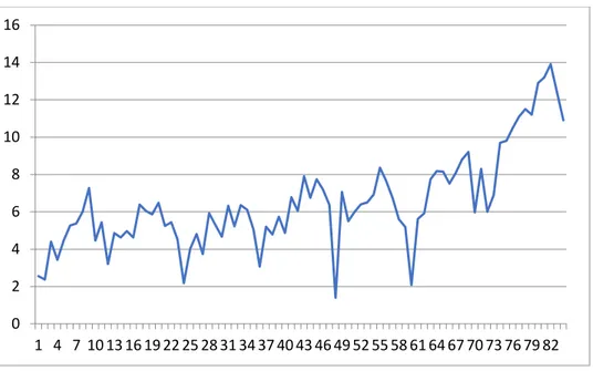
Figure 5. 1 - Yearly demand (Units) aggregated for all products. ...39
Figure 5. 2 - Yearly demand (Units) aggregated for all products and years. ...39
Figure 5. 3 - Aggregated trend (Units) aggregated for all products throughout the years. ...40
Figure 5. 4 - Graphic representation of the mean inter-demand interval (p). ...42
Figure 5. 5 - Representation of products based on (p, CV2) and optimal forecasting method. ..44
Figure 5. 6 - Representation of products based on (p, CV2) and optimal inventory distribution. 50 Figure 5. 7 - Algorithm to find the reorder point. ...52
1
1. Introduction
This chapter presents a degree project that is performed at TitanX Engine Cooling AB in production management. First the general background of the problem will be introduced, followed by the problem description, purpose of the project, company overview, research questions, research limitations, and potential contributions to knowledge will also be explained.
1.1. Background
TitanX manufacturing facilities are designed and operated with a strong and continuous application of lean manufacturing principles, and they perceive themselves as a very flexible supplier. The production sites have a high level of vertical integration, including the manufacturing of key critical components to ensure the highest quality results. The production operations are continuously adjusted to meet variations in customer demand. The vision is to be the number one global supplier of powertrain cooling solutions to the commercial vehicle industry.
The company has three distinct types of customers which are Original Equipment Manufacturer (OEM), Original Equipment Supplier (OES) and Independent AfterMarket (IAM).
● The OEM segment is the biggest in terms of demand, and it consists of finished cooling systems sold to a number of manufacturers to be used in their production of new trucks. The demand for these customers is high and repetitive and it is known well in advance. Orders from these customers can thus be made-to-order.
● The products in the OES segment are spare parts (mostly chargers and radiators) sold to the same customers as the previous segment (OEM). The demand in the OES have a lot of resemblance to the OEM segment and are thus easy to plan.
● Finally, the customers in the IAM segment also orders spare parts, but they are very different than the OES customers. IAM customers are independent distributors that sell the spare parts to smaller truck repair shops. Due to the smaller nature of the customers in this segment, order sizes are usually smaller and more unpredictable, making them harder to control.
The facility in Mjällby consists of three zones; a raw materials warehouse, a shop floor, and a finished goods warehouse. TitanX generally keeps high inventory levels of raw material and finished goods. An important reason for this is the marketing strategy to increase the current market share above 30% of the independent aftermarket for truck engine cooling systems. High customer service levels and good availability are key to achieve this.
2
1.2. Problem description
To figure out what are the challenges of the company that can be the focus of this project, the supervisors at the TitanX factory in Mjällby were approached, and the collected information is provided.
When a customer places its order, TitanX is committed to ship those products within 14 days. This time span is defined as an order to delivery lead time. However, the company is often able to supply the products before the requested time. In fact, most products can be sent immediately and in larger quantities than ordered, even though when an additional amount is shipped with the regular order, the sales department will need to offer a discount. On the other hand, if they cannot ship the items in 14 days, this might cause penalties and/or lost sales.
TitanX also measures dock to dock lead time, this refers to the time an item spends in the system from the time it enters as raw material until it is shipped as a finished good. Today, dock to dock lead time is much higher than the time for order to delivery. The average value for dock to dock lead time is 86 days in total, respectively; 52 days in the raw material warehouse, 19.6 hours of work-in-process, and 33 days in the finished goods warehouse. It is sensed that the total time in the system (86 days) quite long, and the total amount of stock is also pretty high. On the other hand, 19.6 hours work in process is often not sufficient. This since inventory buffers between operations provoke halting of the job and longer time as work in process. Those numbers represent the averages, however, TitanX keeps both OEM and aftermarket stocks. The demand for aftermarket products is rising, moreover, the company sells high variety of the aftermarket products to different distributors. Hence, TitanX would like to have a better understanding of appropriate inventory levels at the finished goods warehouse to meet for the increasing sales of aftermarket products.
The increasing interest of the company in its Independent Aftermarket (IAM) segment started during the 2008 crisis when a new source of income was needed in order to compensate for the decreasing demand tendencies at the time. A new sales team was created to launch this product segment to market and to make it grow. The sales team is making a good job and this segment is continuously growing. Currently, the company wants to increase the ratio of offered IAM products from 65% of their potential market to a goal of 80%, increasing their market share until stabilizing at a desired value of 35% of the global market. These ambitious goals will not come without growing pains in the supply chain of the company.
The Independent Aftermarket (IAM) segment, entail added difficulties compared to the original range of customers. Here are several of the issues that define this new market:
● Customers do not place their orders well in advance, but rather when they need the products.
3
● The market has not stabilized yet. New customers are appearing and demand in general is still in a growing stage.
● Smaller customer orders.
● Quick response (14 days) is expected
Thus, demand needs to be forecasted and stock must always be at hand.
In terms of production, IAM orders introduce many challenges to the company. If one tries to match the customer orders with production orders, productivity issues will arise. This is due to an increase of the total number of setups which will also make production planning harder to optimize. Also, the fact that many products sold in the IAM segment are quite old means that older and more manual machines need to be used, resulting in extra time for the operators and, for the same reason, decreasing part standardization, making production even more complex. Finally, in terms of inventory management, this relatively new branch of products is also introducing new challenges due to the need of forecasting methods, the space constraints caused by the consistent growth in demand and the inventory control difficulties created by the increasing number of offered products.
To comprehend the problems correctly a cause-effect diagram was drawn as seen in Figure 1.1.
4
1.3. Purpose
The purpose of the degree project is to analyze the finished goods inventory for independent aftermarket products to provide both more accurate forecasting methods and a scientific approach for controlling these inventories by finding the reorder points for a given service level and considering trade-offs between the production lead times and the safety stock needed for those.
1.4. Research questions
The research questions of the thesis are the following:
● RQ 1. How to forecast the demand of the products sold in the independent aftermarket segment with sporadic patterns?
● RQ 2. How to control inventory levels of the same group of products?
1.5. Research limitations
As it can be inferred from the research questions, this project will limit its scope to what the company calls Independent Aftermarket products. This is because the spare parts sold to the IAM customers currently use very rudimentary and intuition based planning methods and their sporadic demand patterns make them especially hard for the company to control. Even though the focus market is challenging, TitanX is enriching the product portfolio to gain a bigger market share because of the profitable nature of the aftermarket products. Another limitation of this project is the consideration of only the (R, Q) inventory policy as well as the order quantities/batch sizes (Q) used by the company.
1.6. Contribution to knowledge
This degree project will have practical contributions by understanding how the company should set the reorder point for these products with very specific characteristics and high variation under fast growing market conditions. To do so, a new forecasting tool specific for this special kind of products will be the focus and contribution provided in this project.
It will also support a more theoretical contribution to the issue of spare part management, since this subject has a limited number of conducted studies, by providing guidance for the application in similar cases as the one being studied of categorization and forecasting methods for erratic and/or intermittent demand products, some of which may also be presenting seasonality.
Finally, on a personal level an improvement in problem-solving skills is expected, especially within mathematical modelling of inventory control problems, and will also acquire project management abilities.
5
2. Methodology
As the need for a systemic approach to help carry out and structure the project’s efforts arises, the merits of a more deductive approach to research in contraposition to the more inductive one, become apparent. Deductive reasoning is the process of reasoning from one or more general statements regarding what is known to reach a logically certain conclusion (Johnson-Laird, 2000); (Rips, 1999); (Williams, 2000), and since the company is interested in finding applicable, empirical results that can improve the current forecast and inventory control systems for IAM products, taking advantage of the already existing literature seems the fastest and safest way to do that. Thus, the inductive task of reasoning from specific facts or observations to reach a likely conclusion that may explain the facts Johnson-Laird (2000) is not going to be the most prevalent in this thesis.
In the following lines, the different methods used during this project will be mentioned and explained. Qualitative approaches will have their representation in the use of interviews, and quantitative ones will have theirs in Mathematical Modeling.
For the reason cited in the first paragraph, this chapter also explains “Operations Research” as the approach used to discretize the project into a sequence of steps to reach the project’s final goals. These steps will be covered in more detail in section 2.1.
Eventually, the methods used to gather the required data will be exposed and expanded upon, to better explain the particularities of their application in this project.
2.1. Research method
To study the illustrated case methodically, a quantitative model-driven empirical research method will be practiced.
Kotzab et al. (2005) explained that quantitative model-driven empirical research deals with real life data as well as situations and offers. The same authors noted that empirical model-driven quantitative research is crucial when more practically relevant problems are considered. It is also emphasized that this type of research can be used to validate operations research models in life supply chain processes. Thus, operations research approach will be applied to solve the
real-6
life problem that was specified in the first chapter. Winston and Goldberg (2004) defined the operations research as simply a scientific approach to decision making that seeks to best design and operate a system, usually under conditions requiring the allocation of scarce resources. Liebermann & Hillier (2001) described all the major phases of a typical operations research (OR) modeling approach as the following:
1. Define the problem of interest and gather relevant data.
In general, OR teams receive the description of encountered problems in an imprecise way. So, primarily it must be studied the relevant system and developed a well-defined statement of the problem. This involves specifying the appropriate objectives, constraints on what can be done, interrelationships between the area to be studied and other areas of the organization, feasible alternative courses of action, and time limits for deciding. This effort enables the developers to find the relevant conclusions of the study.
The important thing to be aware of is that an OR team needs to work in an advisory capacity. This means that team members are considered not only as problem solvers but also as advisers of the company’s management team. Therefore, the team should analyze the problem in detail and then present the recommendations. The report will determine the alternatives that are specifically attractive under different assumptions or over a different range of values of some policy parameters that are comprehensible only for managers. Management will make the final decision through evaluation of the study and the recommendations considering a variety of intangible factors. Thus, the OR team must agree on the same perspective with managers to build a support for the improvement.
Data collection can be considered as an initial phase to provide the mathematical model. Much of the needed data will not be available at the beginning of the study, since it is possible that required data never has been kept or data at hand is outdated or kept in the wrong form. Thus, it is recommended to install a new computer-based management information system to gather required data continuously and in the needed form. On the other hand, the OR team may face too much available data, so that it is measured in gigabytes or terabytes. Under this circumstance, a technique that is called data mining would be a solution to process the relevant data.
2. Formulate a mathematical model to represent the problem.
Once the decision maker defines the problem, the next phase will comprise the reformulation of the stated problem in a form that is convenient for analysis. Usually, the OR approach is to develop a mathematical model that reflects the essence of the problem. Mathematical models refer to idealized representations, including mathematical symbols and expressions like F = ma in physics. The mathematical model for a business problem also describes the essence of the problem with the system of equations and related mathematical expressions.
Basically, mathematical models contain decision variables, an objective function, constraints and parameters. If there are n related quantifiable decisions to be made, decision variables (say, x1,
7
x2, …, xn) are used to represent those values that need to be determined. The measure of
performance will be expressed as a mathematical function of these decision variables (e.g. P = x1
+ 3x2 + … + 5xn), and it is called objective function. If there is any restriction on the values that
would relate to these decision variables they are mathematically expressed with inequalities or equations (e.g. 2x1 + 4x1x2 + 6x2 ≤ 8 and these kinds of expressions for the restrictions often
are called constraints. The constants in the constraints and the objective function are named as the parameters of the model. The mathematical model might then indicate that the problem intents to choose the values of the decision variables to maximize the objective function subject to the specified constraints.
Model building can be started with a very simple version, and then it can be modified toward more elaborate models to reflect the complexity of the real problem. This process is called model enrichment and lasts if the model remains tractable.
3. Develop a computer-based procedure for deriving solutions to the problem from the model.
In OR study, the model formulation phase will continue with developing a procedure (usually a computer-based procedure) for deriving solutions to the problem from the model. This step might be considered relatively simple, since a proper algorithm of OR is applied in one of the available software packages. The OR study investigates an optimal or best solution; however, it must be noted that the optimal solution is valid only with respect to the model being used just because the formulated model represents the idealized form of the problem. Therefore, it is not guaranteed that the optimal solution for the model will be the best possible solution to implement for the real problem. However, once the model is well formulated and tested, it will give a resulting solution that offers a good approximation to an ideal course of action.
After finding an optimal solution, postoptimality analysis should be conducted. This process is sometimes verbalized as what-if analysis because it is an ongoing process based on the following question, what would happen to the optimal solution if different assumptions are made about future conditions. Moreover, sensitivity analysis is considered as part of the postoptimality analysis to determine which parameters of the model are most critical. Those sensitive parameters of the model require exceptional care to avoid distorting the output of the model.
4. Test the model and refine it as needed.
When a large mathematical model is developed, it must be expected to develop a large computer program in some way. The initial version of the computer program naturally contains many bugs, so it must be tested successively to seek out and correct as many of them as possible. At the end of the continuous improvement process, the programmer needs to feel that the final program is giving reasonably valid results. Of course, some minor bugs may not be detected, however, the major bugs have been eliminated and hence the program can reliably perform.
8
In addition to bugs, the initial version of the computer program typically contains many flaws that originate from relevant factors or interrelationships which have not been incorporated into the model. Furthermore, some parameters that are accounted inaccurately will also cause the flaws. Thus, before applying the model, it must be tested carefully to detect and eliminate as many flaws as possible. Once the model is improved sufficiently, the OR team can claim that the current model is now giving reasonably valid results. This testing and improvement process is commonly called model validation. The model validation process differs depending on the nature of the problem at hand and the formulated model. However, the OR team would start the model validation with an overall observation to check the model for obvious errors or oversights. It is recommended that the controlling group should include at least one individual who did not participate in the model building process. The definition of the problem might be reexamined and further it can be compared with the model to reveal the mistakes. It should also be considered whether all the mathematical expressions are dimensionally consistent in the units used. Lastly, the model can be validated through changing the values of the parameters and/or the decision variables while observing the model behavior.
5. Prepare for the ongoing application of the model as prescribed by management.
When the testing phase has been completed with an acceptable model, it must be installed a well-documented system for applying the model as prescribed by the manager which helps to use the model repeatedly, which will consist of an instruction handbook with the steps for application as well as explanations of the components found in the input and output interfaces. The required system will consist of the model, solution procedure (including postoptimality analysis), and operating procedures for implementation. This system be computer-based. Indeed, several computer programs often need to be used in harmony, such as databases and management information systems may contribute up-to-date input to run the model each time. One another program is applicable to the model for generating the implementation of the results automatically. In other cases, a decision support system can be installed to help managers use data and models while supporting the decision-making process. It also exists a program to create managerial reports that interpret the output of the model and its implementations for the application.
6. Implement.
When a system is developed for the model, the last phase of an OR study will be the implementation of the system as prescribed by management. The benefits of the study are only occurred here, so that the OR team should participate into the implementation phase to check how the model solutions are accurately translated to an operating procedure and to eliminate any flaws in the solutions that have not handled yet. To carry out this phase successfully, the OR team needs to gain the support of both top management and operating management. Therefore, the OR team should inform management and further encourage the management’s active guidance throughout the course of study to ensure that the study matches with their requirements and they have a greater sense of ownership.
9
The following steps can be used for the implementation phase. First, the OR team explains to operating management how the new system will be adopted and how it relates to operating realities. Then, both parties need to collaborate to develop the procedures required to put this system into operation. After that, operating management monitors that a detailed indoctrination is given to the personnel involved, and the new course of action is initiated. If the new system works successfully, it may be used for years in the same form. Although the system works well the OR team must track the initial experience with the course of action taken to find required modifications that should be attained in the future.
2.2. Quality Assurance
In the previous section, it is explained how to test the model as part of the OR approach. Nevertheless, this assessment should be elaborated in detail having both a verification and validation plan.
2.2.1. Validation
Validation is executed when the developers need to compare the behaviors of the model and the real system. Thus, this process allows to make some adjustments through comparison of the real system and the model. Banks et al. (2005) emphasized a three-step approach for the validation process:
1. Build a model that has high face validity. In this study, the model will be developed in Excel environment, therefore it is possible to illustrate the input and output clearly.
2. Validate model assumptions. It will be done through observation of real scenarios and if
time allows it, by statistical testing. Required assumptions will be specified in the following chapters.
3. Compare the model input-output transformations to corresponding input-output transformations for the real system. This approach will be applied for analyzing the
results of the model.
2.2.2. Verification
Model verification enables the developers to assure if the conceptual model (representation of real system) is reflected accurately in the operational model (computerized representation). The conceptual model usually comprises some degree of abstraction regarding system operations or some amount of simplification of actual operations. Therefore, it should be investigated whether the conceptual model (assumptions about system components and system structure, parameter values, abstractions, and simplifications) is represented properly by the operational model. (Banks et al., 2005)
10
The same source provided the following considerations to verify the model that will be developed in this study. The only consideration that will not be used is verifying that what is seen
in the animation imitates the actual system, due to the operational model not being animated.
1. Have the operational model checked by someone other than its developer. The model is going to be shown to the supervisors at the company throughout the project.
2. Make a flow diagram that includes each logically possible action a system can take when
an event occurs, and follow the model logic for each action for each event type. A full
decision making diagram of the inventory control model will be prepared.
3. Closely examine the model output for reasonableness under a variety of settings of the
input parameters. Have the implemented model display a wide variety of output statistics, and examine all of them closely. Reasonableness will be examined by comparing the
model outputs with current numbers together with the company expertise. Moreover, the model behavior will be observed multiple times with the applications of different adjustments over input data and coefficients.
4. Have the operational model print the input parameters at the end of the simulation, to be
sure that these parameter values have not been changed inadvertently. The input
parameters will be kept in an Excel worksheet (Appendix I).
5. Make the operational model as self-documenting as possible. Give a precise definition of
every variable used and a general description of the purpose of each submodel, procedure (or major section of code), component, or other model subdivision. During the
model building process each variable, submodel and procedure will be defined within the program.
6. The Interactive Run Controller (IRC) or debugger is an essential component of successful
simulation model building. The debugging tool will be used to check if any errors exist.
Besides the code can pause to check the status of the variables.
7. Graphical interfaces are recommended for accomplishing verification and validation.
The graphical representation of the model is essentially a form of self-documentation. It simplifies the task of understanding the model. The interface is an Excel file that shows
the input and output data as well as buttons to choose the confidence interval for the forecasted values, and to run the code.
2.3. Data collection
2.3.1. Interview
11
with respect to interpreting the meaning of the described phenomenon; it will have a sequence of themes to be covered, as well as some suggested questions (Kvale, 2011). To understand the current forecasting and inventory control system of the case company, semi-structured interviews will be conducted together with the following departments: logistics and supply chain, production and sales.
The procedure by Kvale (2011), is the following:
1. Setting the interview stage (briefing)
Creation of an environment in which the interviewee feels comfortable to explain their point of view. It is done by allowing them to have a grasp of the interviewer and the nature of the conversation, and by the interviewer showing respect and interest and listening actively.
2. Scripting the interview
Development of two lists of questions: one with the project's main research questions in academic language, and another with the research questions translated into interview questions that can be understood by the interviewee.
3. Conducting the interview
The interview must have a sequence of themes to be covered as well as some prepared questions, yet at the same time, there should be openness to changes of sequence and question forms to follow up the answers and stories given. At the same time the quality of the interview relies on the interviewer’s ability to apply different techniques such as allowing a pause for the interviewee to continue an answer, probing for more information and attempting to verify the answers given.
4. Analysis of results
Finally, notes or other material obtained from the interview must be analyzed and relevant conclusions must be drawn.
The interviews conducted throughout the project with the purpose of data collection, will mainly be using a semi-structured style and sometimes unstructured. For the semi-structured case, the following steps will be used most often:
Preparation of the interview:
1) Scripting the interview by preparing which questions to ask and which language to use. 2) Prioritization of questions by putting first those questions with higher importance. 3) Setting up premises for the interviewee to know what type of answers are expected from
him.
12
4) Actively listening and showing respect towards the interviewee.
5) Asking questions simultaneously between the two interviewers with room for improvisation.
6) Allowing the interviewee to lead the conversation towards other topics if deemed interesting.
Debriefing of the interview:
7) Further discussion between the interviewers to agree on conclusions.
2.3.2. Direct observation
Direct observation is a method of collecting evaluative information in which the evaluator watches the subject or activity unfold in its usual environment without altering it (Holmes, A. 2013), and will be carried out by visiting the TitanX production facilities in Mjällby.
The procedure is the following:
1. Planning
Preparation of an observational form, allowing the observer to record the occurrence of different activity categories. This must be done after a period of unstructured observation to have a good grasp of the situation.
2. Observation
During this step, the observer must write down or capture in some way all the relevant information for further analysis.
3. Data analysis
Treatment of the raw data from the direct observational studies, for example by counting frequencies or durations of different activities.
2.3.3. Literature review
A literature review is an account of what has been published on a topic by accredited scholars and researchers (Taylor, D., & Procter, M. 2008).
The procedure is explained by Liston, K. (2011) in the following lines:
1. Find resources related to the topic of interest
Sources of information must be obtained regardless of format impact or presentation of the information.
2. Exploration
During this step, the found resources must be read and relevant information must be outlined, structured and analyzed.
13 3. Focus review
Discussion of the scope of the research and contributions to the work.
4. Refine review
Documentation and organization of the information used, and explanation of how the review has affected the project’s research.
2.3.4. Data provided by the company
For this type of data, the company will provide the information already collected and stored in their databases during the last two years (2015 and 2016). The processing of the information into understandable structures for further use will be carried out using different approaches.
One of them will be data mining from the company’s main software to extract valuable data sets for further use in the project. This process will be carried out by the supervisors at TitanX. Once this information has been extracted, another approach that will be used is the manual check of the data found in the excel files which will be further explained in the empirical data chapter. The purpose of this second approach is the elimination of errors and the adjustment for possible missing data.
Finally, another approach will be the use of Python programming language to prepare data for its later use in the forecasting tool.
15
3. Theory
The theory chapter is divided into two main groups; forecasting and inventory control. Particularly, forecasting has a focus on items with intermittent demand pattern, while inventory control covers the single echelon systems. Forecasting will be used to provide a better insight on the demand patterns that the different IAM products are expected to have as well as to feed the inventory control tool created in this project and inventory control will be used to know the different reorder points as well as to gain better insight on the leverage of lead times compared to the necessary safety stocks to meet the desired service levels.
3.1. Forecasting
For this project, several forecasting approaches have been taken into consideration, such as the use of Bootstrapping methods reviewed by Smith, M., & Babai, M. Z. (2011) or the use of neural networks (Kourentzes, N., 2013). These are not going to be explained because of their complexity and lack of relation to this project. A categorization procedure for forecasting purposes was chosen as it is an alternative that has been studied and reviewed by many authors. For instance, Bucher and Meissner (as cited in Altay and Litteral, 2011), provide a satisfactory performance for the group of items that is being studied and is accessible to the company in terms of its simplicity.
In this chapter, demand categorization schemes are explained first. The one used for this project is expanded and its parameters and their respective calculations are also shown. Next, a five-step process for the implementation of a demand categorization scheme is presented, the possibility of seasonal and trended demand patterns is considered and finally, the chosen forecasting methods are mentioned together with their procedures and formulas.
3.1.1. Demand patterns
The company was interested in analyzing the historical demand data of their products to find possible patterns that would give a better understanding of them as well as to improve the accuracy of the forecast and inventory control tools being developed. Mainly two types of patterns were expected by the supply chain team: seasonal effect and trend.
Seasonality is a repeated pattern of spikes or drops in a time series associated with certain times of the year (Bozarth and Handfield, 2008). Time-series plots, seasonal subseries plots, box plots
16
and autocorrelation plots will also be used as they help visualize seasonal patterns (6.4.4.3. Seasonality, 2017).
Trend represents a long-term movement, up or down, in a time series. (Bozarth and Handfield, 2008). For this case, the same analysis as the one explained in the previous paragraph is carried out.
Aside from those items with the special demand patterns mentioned in the previous paragraphs and where alternative methods and more careful attention will be required, Bucher, D., & Meissner, J., (2011), authors of the five-step process for the implementation of a demand categorization scheme explained in the following paragraphs, noted a configuration of the forecasting categorization scheme which considers four different patterns based on the mean inter-demand interval (p) and squared coefficient of variation of the order sizes (CV2),as seen in
Figure 3.1:
Smooth: Short time between orders and low variance of the order sizes. Slow: Long time between orders and low variance of the order sizes. Erratic: Short time between orders and High variance of the order sizes. Lumpy: Long time between orders and High variance of the order sizes.
As you can see in Figure 3.1. smooth and erratic categories have more demand points in historic data, conversely slow and lumpy ones have many periods with zero demand. In addition, the similar structure exists for demand variation where high variation occurs for erratic and lump categories as well as more consistent demand size for smooth and slow products.
17
3.1.2. Demand segmentation
The classification of the various products within the portfolio of a company is a topic that has attracted many studies in the past. The main objective here is to help identify the regions that differ in suitable method for forecasting in order to improve the forecasts which in turn should lead to cost reductions and/or service level improvements.
One of the first categorization schemes, and still to this day a very popular one, is the ABC-analysis (Dickie, 1951), that classifies products in one of three categories (A, B or C) in a decreasing fashion, according to the benefit they report to the company or the size of the demand. This analysis is currently being used in the company with the purpose of prioritizing the production of the different items and will also be used later in this project to obtain the production lead times of the various products as shown in the empirical data section of chapter 4. Even though ABC analysis is applicable for demand pattern categorization, it is not the main purpose of this method, since it does not consider any information regarding demand patterns, but it is mentioned as a precursor to other categorization schemes that appeared during the decades after.
Williams (1984) was the first author to examine intermittent demand patterns in his categorization by using the concept of variance partition. In his work, he calculates the squared coefficient of the variation of demand during the lead time as seen in Equation 3.1
(3.1)
where L: lead time; : squared coefficient of demand size variation during the lead time; CV2: the squared coefficient of variation of the distribution of the demand sizes; λ: Mean number of arrivals per time unit.
The first term represents the mean number of lead times between demands whereas the second term relates to the lumpiness of demand, and both parameters are later used to categorize a product sample.
Johnston and Boylan (1996) showed that the Croston forecasting method outperforms the exponentially weighted moving average (EWMA) method robustly over a wide range of parameter settings, when the average inter-demand interval is greater than 1.25 forecast revision periods. This study showed the importance of intermittence as a parameter to consider when setting up a categorization scheme for your products.
Eaves (2002) took the categorization made by Williams one step further, adding a parameter to consider lead time variability. Since then, lead time variability has remained as a topic for further research.
18
Finally, the categorization used in this project is the one by Syntetos et al. (2005), who were the first to create a categorization scheme close to achieving universal validity, using the inter-demand interval (p) and the coefficient of variation of the inter-demand size (CV2), which will be touched on later (not to be confused with from Williams (1984)).
Formulas of p and CV2 can be seen in Equation 3.2 and Equation 3.3. The calculation of p is an approximation used by the authors of this project based on the interpretation of the same article and is explained in the following lines (n: number of periods with demand; ti: period i=1...T; σ:
standard deviation; µ: mean).
(3.2)
(3.3)
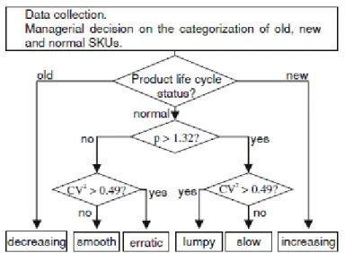
Bucher, D., & Meissner, J., (2011) developed the basic steps for the implementation of a demand categorization scheme. This framework is especially interesting for organizations that keep a high number of SKUs and so desire to increase both the level of automated inventory management and the overview of their inventories, by grouping spare parts using factors in line with a single-echelon system configuration. The following five steps are defined to be a guide especially for the considerations of categorization. The framework for the implementation of a categorization scheme can be seen in Figure 3.2.
Figure 3. 2 - The framework for the implementation of a categorization scheme (Bucher, D., & Meissner, J., 2011).
1. In this step, the historic demand data should be collected for all SKUs of the spare parts inventory. Commonly, this information can be gathered from reports of the corporate ERP system.
2. The authors formed the first categorization factor by considering the status of an item in the product life cycle and those are normal, new and old SKUs. The reason is to
19
differentiate new and old SKUs as they are usually very difficult to predict with parametric forecast. Then they would be managed either manually or with other best practice methods. On the other hand, distinguishing each SKU is a time consuming manual process. Thus, a factor can be assigned, such as the cumulative demand of the last 12 months might be compared to the cumulative demand of the last 36 months to detect either decreasing or increasing demand trend. Lack of historic demand records indicates that it might be a newly introduced item.
3. When the normal SKUs differentiated from new and old ones, the average inter-demand interval p and the squared coefficient of variation of demand size CV2 can be determined from historic demand data for each item.
4. The values that are calculated in the previous step will be used to categorize the SKUs according to the illustrated scheme. Afterwards, the single-echelon inventory system can be configured for each SKU with respect to the assigned methods.
5. Eventually, it is recommended to re-group the products on a yearly or a more frequent basis. This process is important to keep the results as trustable especially when SKUs change over from new to normal and from normal to old.
3.1.3 Forecasting methods
The forecasting methods for a categorization scheme of intermittent demand products recommended by Bucher, D., & Meissner, J., (2011) are Croston and the Syntetos and Boylan Approximation (SBA). The methods chosen in this project will be motivated during the analysis chapter.
In the following lines, the theoretical iterative processes for the different forecasting methods used are explained.
Croston and SBA method:
Step 0: Initialization of the process using the first τ periods.
For initialization purposes, the initial value for the size of the estimated demand ( ), is equal to the initial value of the mean demand ( ) which is calculated as the mean demand size of the periods where demand has occurred, only considering the first τ periods. The initial value of p ( ) is also the one calculated for the first τ periods. Finally, q is the time until the next demand during the current iteration, and is initialized to zero. ; ; ; If there is no demand then ; 1; ;
Step 1: Start of the iterative method at period τ +1 (until period T). For period t = τ +1 to T:
20 Else:
where and denote the estimates of inter-demand interval and demand size. Step 2: Forecast.
Once and are obtained, the iteration ends. Finally, the forecast in units/period ( ) is defined in Equation 3.4 and Equation 3.5 are calculated:
● Croston: (3.4)
● SBA: (3.5)
where α: smoothing coefficient; : forecast in demand/period.
Simple Exponential Smoothing (SES):
Step 0: Initialization (Using the first month)
The output of the first iteration of the SES algorithm ( ) will be equal to the demand of the first period.
Step 1: Iterative method.
The forecast for the following periods will be calculated with Equation 3.6:
(3.6)
where and denote the forecast and the real demand in period t. Further, again refers to the smoothing coefficient.
Step 2: Forecast.
Once the iterative method ends, the demand forecast for the next period as well as variance (as seen in Equation 3.7) are calculated:
(3.7)
21
On the other hand, the company believes that products with a certain increasing/decreasing trend as well as seasonality exist within the company’s aftermarket portfolio. The Holt-Winters method is a promising option to forecast these products since it adapts to both additive and multiplicative seasonality and/or trend, all in one method. Additive seasonality or trend for monthly data assumes that the difference between the January and July demand values is approximately the same each year, while the multiplicative case impliesthat the July value is the same proportion higher than the January value in each year (Time series forecasting: understanding trend and seasonality, 2014). The analysis conducted in chapter 5 proved that there is no perceivable seasonality and that there are a very limited number of products with a trend pattern. Therefore, the application of this method is not necessary for this project.
Aggregation level
In addition to the application of the methods, and to improve their performance, following recommendations by Nikolopoulos et al. (2011), for each data set there is a certain level of aggregation of the data into time buckets which may improve forecast accuracy. For example, the same authors recommend the review period plus the lead time as a promising alternative, since in a practical inventory setting, it would make sense to set this aggregation level, as cumulative forecasts over that time horizon are required for stock control decision making (Nikolopoulos et al., 2011).
To be able to compare errors for different aggregation levels, Axsäter (2006) suggested Equation
3.8. If the assumption of normal distribution of the forecasting errors is accepted, Equation 3.9 is
valid (Axsäter, 2006) and therefore Equation 3.8 can be applied for the case of MAD resulting in
Equation 3.10. Therefore, if the effects of auto-correlation are not taken into consideration,
monthly MAD can be converted to weekly dividing by .
(3.8)
(3.9)
(3.10)
Exponential smoothing coefficient (α)
Axsäter (2006), recommended the use of Equation 3.11 to calculate the smoothing coefficient, which implies that α changes based on the aggregation period, as, for example, a data set of 12 months (N=12) will now have an N of 52 if the aggregation is changed from monthly to weekly.
(3.11)
22
By using Equation 3.11 the average age of the used data is ensured to be the same for both SES and Simple Moving Average (SMA) forecasting procedures with a rolling horizon of N (Axsäter, 2006).
It is also important to note that a smaller α has the effect of putting relatively more emphasis on old values of demand.
Forecast accuracy
The most common way to describe variations around the mean is through the standard deviation (σ). In the case of forecast errors, the widespread practice by most of the forecasting software is to use the Mean Absolute Deviation (MAD), as seen in Equation 3.12 calculated as the expected value of the absolute deviation from the mean. This tradition came from the fact that originally, MAD simplified the computations in comparison to other estimators like σ and σ2
. Nowadays, this is not the case anymore, but due to MAD and σ giving a very similar picture of the variations of the mean in most cases, a need for change has not appeared. (Axsäter, 2006).
(3.12)
Aligning with the conventional procedures in this field, the measurement of forecasting error used will also be MAD.
3.2. Inventory control
According to Axsäter (2006), an inventory control system has a function to determine when and how much to order. It considers the stock situation, the anticipated demand and different cost factors. Therefore, this section will cover primarily different ordering systems, followed by the single echelon systems in terms of resolving the reorder points. It should be noted that this study does not cover determination of the batch size since a certain batch size has already been assigned to each product by TitanX.
A suitable safety stock or reorder point can be determined based on either a prescribed service constraint or a certain shortage or backorder cost. Service level can be defined differently: (Axsäter, 2006)
S1= probability of no stock out per order cycle,
S2= "fill rate"- fraction of demand that can be satisfied immediately from stock on hand,
23
The first definition of service level (S1) does not take the batch size into account. Therefore, it
might not be able to represent the real service level or situation.Instead, in this study, a sufficient reorder point R is investigated to satisfy a given ready rate S3 (which in the cases of Normal,
Poisson and Gamma distributions will be equal to the fill rate S2 according to Axsäter (2006)). It
must be recalled that a continuous review (R, Q) policy is the concern in this study and further the batch quantity Q for each item is given by the case company.
3.2.1. Different ordering systems
According to the 5-steps framework for the categorization of intermittent demand patterns described in section 3.1.2, the periodic review system is recommended for all categories even though other systems are also applicable. Moreover, the dynamic (t, S)-policy will naturally be the choice considering the context of spare parts management, where the order-up-to level S needs to be recalculated in every order period (t) in which demand occurs. Meanwhile, in general the selection of the order-policy does not affect significantly to the inventory performance for intermittent demand. (Bucher, D., & Meissner, J., 2011)
In this section, different ordering policies in terms of continuous and periodic review will be explained. Specifically, continuous review and (R, nQ) policy will be elaborated more in detail, since that is the desire of the company.
Continuous or periodic review
An inventory control system can be designed based on either continuous or periodic review. Before emphasizing the difference between the two, it is necessary to describe the inventory
position and the inventory level. Normally the stock situation implies stock on hand, however,
when it comes to an ordering decision, it should also be regarded the outstanding orders that have not yet arrived, and backorders. This explains why the stock situation needs to be represented by the inventory position. (Axsäter, 2006)
It is illustrated as seen in the following expression:
A parenthesis can be opened here for the event that the customers can reserve units for later delivery. This reserved units should be subtracted from the inventory position unless delivery time is too distant. Inventory position is related to make ordering decisions, but instead the inventory level becomes applicable to reveal holding and shortage cost. (Axsäter, 2006)
It is formulated:
24
For some cases, the holding costs should also include holding costs for outstanding orders. This would be easily obtained as the average lead time demand. (Axsäter, 2006)
After a brief explanation of the inventory position and the inventory level, we can return to the review systems. The continuous review system refers that the inventory position is monitored continuously and when it is sufficiently low an order is triggered. This order will be delivered after a lead-time which starts once the ordering decision has been made and finishes when the ordered amount is placed on a shelf. Along with the transit time from an external supplier or the production time for an internal order, the lead-time also contains order preparation time, transit time for the order, administrative time at the supplier, and time for inspection for the received order. (Axsäter, 2006)
Alternatively, the inventory position can be assessed only at certain given points in time. This approach is called as periodic review and it offers advantages, especially when it is needed to coordinate orders for different items. Besides, periodic review helps to reduce the costs for the inventory control system specifically for items with high demand. But since the case company evaluates the inventory level several times within a week, continuous review will prevail in this study. Furthermore, it is common to use continuous review for items with low demand in practice and it reduces the needed safety stock. (Axsäter, 2006)
Different ordering policies
Axsäter (2006), expressed the two most common ordering policies about inventory control, namely (R, nQ) and (s, S) policy. The case company prefers to use the (R, nQ) policy since it has been an exercised method until today. As a required alternative, this policy is chosen to build an inventory control solution.
The reorder point-R regulates the ordering decision, meaning that when the inventory position declines to or below the reorder point R, a batch quantity of size Q is ordered. In case that the inventory position is dramatically dropped, it may be necessary to order more than one batch to get above R. (Axsäter, 2006)
The second policy is also like the (R, nQ) policy. Now the reorder point is represented by s and when the inventory position decreases to or below this number, it is ordered up to the maximum level-S. If the reorder point is hit exactly (continuous review and continuous demand), the two policies can be considered as equivalent provided s = R and S = R + Q. (Axsäter, 2006)
3.2.2. Single-echelon systems determining reorder points
The purpose of this study is developing a model to find the reorder points or safety stocks for a given service level, which helps to test the effect of different service conditions on safety stock. Furthermore, with an inventory control model, reorder points can be evaluated for lead-time changes easily. To formulate this problem, the demand distribution of the products must be
25
shown. In forward part, inventory level distributions will also be described since it is needed in the service level calculation.
Demand distributions
Axsäter (2006) suggested the use of different theoretical demand distributions to model the real demand distributions seen for each of the products.
The demand during a certain time is a discrete stochastic variable as it is nearly always a nonnegative integer. If the demand is reasonably low, it is then natural to use a discrete demand model, which resembles the real demand. On the other hand, when the demand is relatively large, it is more practical to use a continuous demand model as an approximation. (Axsäter, 2006)
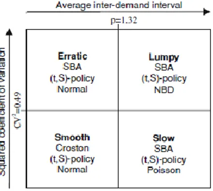
According to Bucher, D., & Meissner, J., (2011), different theoretical distributions are recommended to approximate the empirical demand distributions. It is expected that the normal distribution will bring a good description of the empirical distributions for the erratic and smooth categories. Furthermore, Boylan et al. (2008) used the Poisson distribution for the slow category and the negative binomial distribution for the lumpy category. Finally, the single-echelon configurations for each category can be seen in Figure 3.3.
Figure 3. 3 - Categorization scheme for a single-echelon inventory configuration (Bucher, D., & Meissner, J., 2011).
For the discrete demand case, first the pure Poisson together with the compound Poisson demand will be described, and later it will be shown the logarithmic compounding distribution. In stochastic inventory models, it is commonly assumed that the cumulative demand can be modeled by a non-decreasing stochastic process with stationary and mutually independent increments. It is possible to represent this process as a limit of an appropriate sequence of compound Poisson processes. Consequently, the demand is often assumed that it follows a compound Poisson process. In depth, the customers arrive corresponding to a Poisson process with a certain intensity Further the size of a customer demand is also a stochastic variable. (Axsäter, 2006)