An explanation to the VTI FILTER documents

(1)

Author

Peter Andrén & Leif Sjögren

Research division Measurement Technology and

Methods

Project number

80250

Project name

Road surface measurement, methods

and necessary accuracy

Sponsor

KFB/VV

Distribution

Free

VTI notat 39A-2001

An Explanation to the

VTI FILTER documents

VTI notat 39A • 2001

0.01 0.1 1 108 107 106 105 104 103 102

Spatial frequency, n (cycles/m)

Displacement po w er spectr al density (m 3) RoadRuf

Matlab code (Device E 23)

0.1 1 10

Angular spatial frequency, Ω (rad/m) 1 10 100 Wavelength, λ (m) 108 107 106 105 104 103 G_d(Ω) G_d(n) FILTER

Section: Q DAF test track 23. Surface: Concrete Section length: 400 m Speed/Run: 60/3

(2)

Foreword

During the cause of the FILTER project the Swedish National Road and Trans-portation Research Institute has been working on a project financed by the Swedish Transport & Communications Research Board and the Swedish National Road Ad-ministration concerning the required accuracy of road measuring devices. In this work we made extensive use of data from the FILTER project, resulting in the doc-umentation found on the Compact Disc. We distribute this material as we’ve found it useful as a tool for browsing through the data, and hope that you will find it use-ful too. Please direct all questions of a technical nature to Peter Andr´en on email

peter.andren@vti.se.

N.B. This documentation is not a part of the official FILTER documenta-tion. The official documentation describing the longitudinal analysis can be found in “FILTER Experiment: Analyses of the Longitudinal Profiles and In-dices” by Ducros, D-M., Petkovic, L., et al.

Link¨oping, 2000-05-18

(3)

1 Introduction

This document explains how to read the PDF documents on the VTI-FILTER CD.

Apart from the “reading instructions” a comparison with the RoadRuf program for the IRI and PSD Matlab functions is included. A small comparison of the calculated IRI for the different devices has also been added at the end of the document. We can see that all devices behave reasonably well in that aspect.

I have analyzed the test section profiles from the original CD from Daniel-Marc Ducros, LCPC. In the case of Device C 15 new profiles were delivered after the test, as some problem had occurred in the post processing (each profile was a cumulative sum instead of the profile). I use the notation Device Code Test Section Speed -Repetition to refer to a certain test profile, e.g. Device D 16 - W - 60 - 3 for the third repetition in sixty on test section W for device D 16.

The work presented in this, and accompanying, documents has been done with Matlab for the number crunching, and pdfLA_{TEX for typesetting and document}

pro-duction. The documents presenting the results from the devices and the Primal were created in one 30 hour Matlab session on May 5, 2000. This Matlab ses-sion created almost 7500 PostScript figures and about 70,000 lines of LA_{TEX code}

in twenty-one documents. Another major computer session converted the figures to the Portable Document Format and compiled the PDF-documents. This resulted in

the twenty-one PDF-documents on this CD, altogether containing more than 5600

pages. Despite the large size of this job both Matlab and pdfLA_{TEX behaved very}

well.

However, due to the vast amount of documentation, I haven’t been able to check all results for errors. If you find anything that’s obviously wrong, very strange or if there’s room for improvements please contact me onpeter.andren@vti.se. Feel free to contact me about other things concerning these documents: if you want the Matlab source code, need more information on some specific detail, or just about anything else. (The Matlab source code isn’t distributed on this CD as it was in a state of ad hoc at the time when the CDs were made. My plan is to comment the

code, remove unused parts and put it in public domain. Mail me if you’re interested in receiving a copy.)

Many thanks to Daniel-Marc Ducros at LCPC, France for many rewarding dis-cussions concerning various details of longitudinal road profile analysis, and other topics as well.

(5)

2 The

DeviceXNN.pdf

documents

On the Compact Disc where this document is found, you can also find 21 documents namedDeviceXNN.pdfwhereXis the group code, andNNis the device number, following the FILTER notation. This document contains an explanation of how to read and understand theDeviceXNN.pdfdocuments.

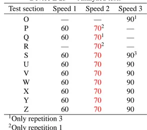
The document starts with a table (as in Table 2.1 below) on the first page giving information on for which test sections and at what speeds the device has delivered data. The normal procedure was that three repetitions were carried out for each speed and test section. If the device in question hasn’t delivered data for any tests that place in the table is marked with a dash (—), and if not all three repetitions were carried out, this is marked with with a footnote comment in the table.

The optimum speed is printed in red. For a few devices (C 11, C 13, F29 and F30) the optimum speed is said to be 99 km/h. This is not necessarily true, as 99 was supposed to be used as a code for the optimum speed. The true optimum speed for these devices should be documented elsewhere.

Table 2.1: Example of Device Information Table. Device E 23 — Analyzed tests

Test section Speed 1 Speed 2 Speed 3

O — — 901 P 60 702 _— Q 60 701 _— R — 702 _— S 60 70 903 U 60 70 90 V 60 70 90 W 60 70 90 X 60 70 90 Y 60 70 90 Z 60 70 90 1_{Only repetition 3} 2_{Only repetition 1}

3_{Only repetitions 1 and 3}

The second table contains a summary of all the tests carried out by the device. The data in this table can also be found at the more detailed presentation further back in the document. The first three columns (denoted TEST INFORMATION) give the test section, the speed and the repetition. The other columns contain results collected in this table for easy comparison. The meaning of the other columns will be explained when the detailed analysis is explained.

(6)

Table 2.2: Example of “All Test Section Table”. See Table 2.4 and 2.5 for the notation.

TEST INFORMATION CORRELATION PIARCRMS FRENCH RMS IRI Road Speed Run Ru Ra l p1 p2 f1 f2 f3 Iv Ip

O 60 1 0.622 0.635 -0.20 0.644 0.081 0.089 0.021 0.052 5.872 5.833 O 60 2 0.607 0.691 -0.50 0.639 0.086 0.094 0.038 0.070 5.889 5.833 O 60 3 0.570 0.598 0.25 0.635 0.109 0.114 0.042 0.038 5.790 5.833 O 75 1 0.299 0.463 0.80 0.641 0.103 0.111 0.039 0.043 5.846 5.833 O 75 2 0.363 0.563 -1.00 0.637 0.098 0.105 0.041 0.027 5.759 5.833 O 75 3 0.561 0.680 -0.65 0.638 0.107 0.098 0.029 0.064 5.705 5.833 O 90 1 0.433 0.438 0.15 0.636 0.120 0.121 0.036 0.056 5.539 5.833 O 90 2 0.091 0.472 2.15 0.639 0.108 0.115 0.036 0.046 5.671 5.833 O 90 3 0.647 0.647 0.05 0.637 0.096 0.111 0.032 0.064 5.720 5.833 P 60 1 0.767 0.790 0.35 0.669 0.102 0.095 0.068 0.088 3.705 3.460 P 60 2 0.863 0.928 -0.55 0.663 0.087 0.081 0.065 0.073 3.709 3.460 P 60 3 0.794 0.847 0.55 0.672 0.088 0.082 0.061 0.068 3.693 3.460 . . . . . . . . . . . . . . . . . . . . . . . . . . . . . . . . . . . . . . . Z 90 1 0.810 0.820 0.60 0.831 0.192 0.137 0.152 0.058 0.901 0.940 Z 90 2 0.799 0.802 0.40 0.754 0.159 0.137 0.135 0.049 0.868 0.940 0.637 0.702 2.28 0.722 0.209 0.174 0.194 0.106

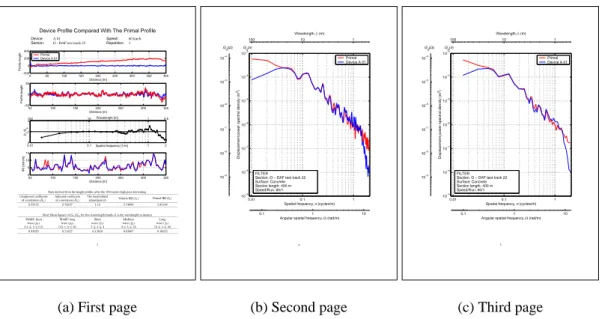
After the two tables follows a more detailed presentation of all the analyzed road profiles. Each and every analyzed profile is presented with a set of three pages, as illustrated in facsimiles in Figure 2.1 (a-c). The first page is made up of three tables and four graphs. The first table, at to the top of the page, gives some general information on the device, test section, speed and repetition analyzed. The top graph shows the two profiles to be compared. The Primal profile is presented just as it was delivered, and the device profile after detrending with a best fit (least-square sense) three-order polynomial. This detrending is carried out to increase the numerical stability in the resampling function.

Device Profile Compared With The Primal Profile

Device: A 01 Speed: 60 km/h

Section: O - DAF test track 22 Repetition:1

0 50 100 150 200 250 300 350 400 −200 0 200 400 Distance [m] Profile height Primal Device A 01 50 100 150 200 250 300 350 −50 0 50 Distance [m] Profile height 0.010 0.1 1 1 2 0.5 2 Spatial frequency [1/m] Wavelength [m] Gv /G p 1 10 100 50 100 150 200 250 300 350 0 5 10 15 Distance [m] IRI [mm/m]

Data derived from the height profile, after the 100 metres high pass detrending. Unadjusted coefficient Adjusted coefficient The longitudinal Vehicle IRI (✂✁

) Primal IRI (☎✄

) of correlation (✆✞✝) of correlation (✆✞✟) adjustment (✠)

0.55325 0.78297 1.10 5.74890 5.83294 Root Mean Square of✡

✁☞☛

✡

✄

for five wavelength bands (✌is the wavelength in metres) PIARC short PIARC long Short Medium Long wave (✍✏✎) wave (✍✒✑) wave (✓✔✎) wave (✓☞✑) wave (✓☞✕)

✖✘✗✚✙✞✛ ✌ ✛✜✖✘✗✢ ✖✣✗✤✢✦✥ ✌ ✛✧✢☞✖ ✙★✛ ✌ ✛✪✩ ✩✫✛ ✌ ✛✬✙✭✩ ✙✭✩✫✛ ✌ ✛✜✮✯✖ 0.95955 0.21627 0.13016 0.03867 0.10023 3

(a) First page

0.01 0.1 1 10−9 10−8 10−7 10−6 10−5 10−4 10−3

Displacement power spectral density (m

3)

Primal Device A 01

0.1 1 10

Angular spatial frequency, Ω (rad/m) 1 10 100 Wavelength, λ (m) 10−9 10−8 10−7 10−6 10−5 10−4 G d(Ω) Gd(n) FILTER Section: O − DAF test track 22 Surface: Concrete Section length: 400 m Speed/Run: 60/1 4 (b) Second page 0.01 0.1 1 10−9 10−8 10−7 10−6 10−5 10−4 10−3

3)

Primal Device A 01

0.1 1 10

Angular spatial frequency, Ω (rad/m) 1 10 100 Wavelength, λ (m) 10−9 10−8 10−7 10−6 10−5 10−4 G d(Ω) Gd(n) FILTER Section: O − DAF test track 22 Surface: Concrete Section length: 400 m Speed/Run: 60/1

5

(c) Third page

Figure 2.1: Facsimiles of one set of pages presenting one repetition (Device A 01 -O - 60 - 1)

(7)

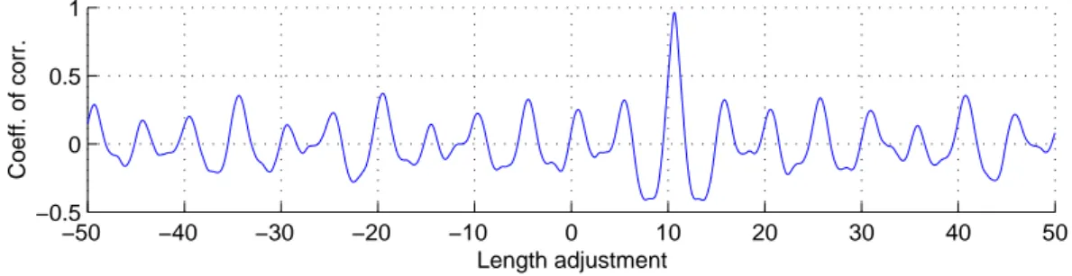
−50 −40 −30 −20 −10 0 10 20 30 40 50 −0.5 0 0.5 1 Length adjustment Coeff. of corr. Figure 2.2: Correlation

In the second graph 50 meters on each side of the Primal profile has been cut off. The device profile is trimmed so thatmaximum correlation between the two

profiles is achieved. The correlation for different positions can be seen in the Figure 2.2. In this example (Device A 01 - P - 60 - 1) the best correlation occurred after about 10 meters, i.e. the test started 10 meters early. This process will make sure that the profile to profile comparisons are as fair as possible.

The coefficient of correlation for the unadjusted and longitudinally adjusted case are presented in the table at the bottom of the page (here Table 2.4). In some cases the adjusted profiles have alower coefficient of correlation than the unadjusted ones.

The explanation to this is that both profiles (device and Primal) are high-pass filtered with a ten meter filter before the maximum correlation is searched (this will focus the search algorithm on shorter, more identifying, wavelengths). However, when the maximum correlation of the longitudinally adjusted profiles is calculated the 100 meter high-passed filtered profiles are used, and the coefficient of correlation might change slightly. This will usually not influence very much, unless the maximum correlation is very low (e.g. Device B 10 - U - 60 - 1/2/3).

The second and third pages (Figure 2.1(b–c)) contains the Power Spectral Den-sity (PSD) functions for the both profiles. These graphs are made according to the ISO 8608 standard [4]. The second page presents the PSD profile for all possible spatial frequencies from 0.01 to 2 (i.e. from 0.5 to 100 meter’s wavelength). The same function smoothed in octave bands for center spatial frequencies up to 0.0312, in third-octave bands from 0.0496 to 0.250, and twelfth-octave bands for the higher frequencies is presented on page three. A quote (usually called transfer function) between the smoothed PSD for the device profile and Primal profile is given in the third graph on Figure 2.1(a).

The last graph in Figure 2.1(a) is the International Roughness Index (IRI) for the profiles. IRI values have been calculated for three meter sections, as this was considered to be detailed but still not too detailed.

The second table at the bottom of page one presents the coefficient of correlation for the unadjusted and longitudinally adjusted profiles, as well as the length of the adjustment. Next, the IRI for the entire profiles are given. The IRI code follows the

Table 2.4: Example of the correlation and IRI table. Data derived from the height profile, after the 100 meters high pass detrending.

Unadjusted coefficient Adjusted coefficient The longitudinal _{Vehicle IRI (}_I

v) Primal IRI (Ip)

of correlation (R_u₎ _{of correlation (}R_a₎ _{adjustment (}l₎

-0.01835 0.45889 10.30 5.79836 5.82452

(8)

recommendations from (a draft version of) Sayers’ article “On the Calculation of

IRI from Longitudinal Road Profile” [9]. A comparison between my Matlab code

and RoadRuf is given in Section 3.

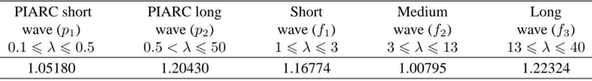
The last table presents a few root mean square values for the transfer function between the two PSD function, i.e. the third graph on page one. TheseRMS values have been divided into five wavelength bands according to the PIARC recommen-dations, and to what in Sweden is called the French wavelength bands. The RMS

computation is done mainly to get a numerical representation of the transfer func-tion.

Table 2.5: Example of the correlation and IRI table.

Root Mean Square ofGv/Gpfor five wavelength bands (λ is the wavelength in meters)

PIARC short PIARC long Short Medium Long

wave (p1) wave (p2) wave (f1) wave (f2) wave (f3)

0_{.1 6 λ 6 0.5} 0_{.5 < λ 6 50} 1 6λ 6 3 3 6λ 6 13 13 6λ 6 40

(9)

3 Comparison with RoadRuf

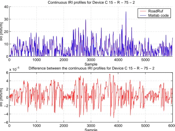
In order to validate the behavior of the Matlab code used a comparison with the RoadRuf software [10] was conducted. A continuous IRI profile (i.e. no averaging over subsections) was calculated with the Matlab code. The road profile (in this case Device C 15 - R - 75 - 2) was then written to theERDformat, analyzed in RoadRuf, and read into the Matlab routine for comparison and plotting. The result was very satisfactory, and is presented in the figure below. As can be seen the two profiles more or less coincide, and the difference between them (in the order of 10−5_mm/m)

can safely be ignored.

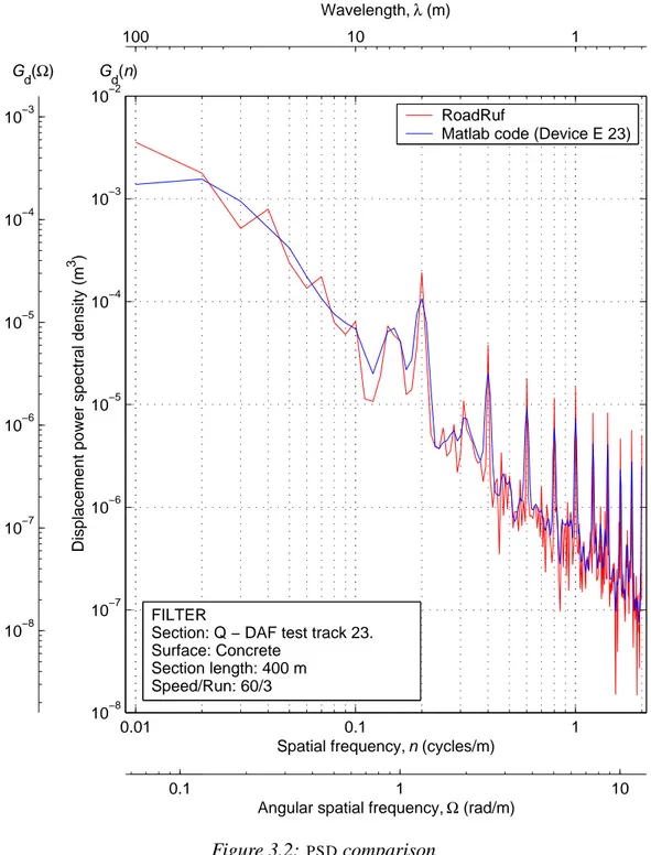
A similar test was carried out for the Power Spectral Density code. The figure on next page shows the result. Again, there’s nothing crucial to complain about.

0 1000 2000 3000 4000 5000 0 10 20 30 40 IRI [mm/m] Sample

Continuous IRI profiles for Device C 15 − R − 75 − 2

RoadRuf Matlab code 0 1000 2000 3000 4000 5000 6000 −6 −4 −2 0 2 4 6x 10 −5 IRI [mm/m] Sample

Difference between the continuous IRI profiles for Device C 15 − R − 75 − 2

Figure 3.1: IRI comparison

(10)

0.01 0.1 1 10−8 10−7 10−6 10−5 10−4 10−3 10−2

3 )

RoadRuf Matlab code (Device E 23)

0.1 1 10

Angular spatial frequency, Ω (rad/m)

1 10 100 Wavelength, λ (m) 10−8 10−7 10−6 10−5 10−4 10−3 G_d(Ω) G_d(n) FILTER

Section: Q − DAF test track 23. Surface: Concrete

Section length: 400 m Speed/Run: 60/3

(11)

4 An IRI comparison for all devices

Ability to measure the IRI is one of the most important features of any road surface measuring equipment. Figure 4.1 below summarizes all the IRI values delivered for all devices at all speeds. As can be seen in the figure all devices produce a similar result. The differences that can be seen are most likely mainly due to the position on the test section more than the capability of the device.

Figure 4.2 on next page illustrates how the different devices have performed on the different test sections. IRI from the Primal is drawn as a red line across the graphs. O P Q R S U V W X Y Z 0 1 2 3 4 5 6 7 8 9 Road IRI A 01 A 02 B 06 B 07 B 09 B 10 C 11 C 12 C 13 C 15 D 16 D 17 D 18 D 19 E 22 E 23 F 27 F 29 F 30 G 32 G 33 Primal

Figure 4.1: IRI comparison

(12)

1 2 6 7 9 10 11 12 13 15 16 17 18 19 22 23 27 29 30 32 33 2 4 6 IRI on O 1 2 6 7 9 10 11 12 13 15 16 17 18 19 22 23 27 29 30 32 33 3 4 5 IRI on P 1 2 6 7 9 10 11 12 13 15 16 17 18 19 22 23 27 29 30 32 33 3 4 5 IRI on Q 1 2 6 7 9 10 11 12 13 15 16 17 18 19 22 23 27 29 30 32 33 6 7 8 IRI on R 1 2 6 7 9 10 11 12 13 15 16 17 18 19 22 23 27 29 30 32 33 0.5 1 1.5 IRI on S 1 2 6 7 9 10 11 12 13 15 16 17 18 19 22 23 27 29 30 32 33 0 1 2 IRI on U 1 2 6 7 9 10 11 12 13 15 16 17 18 19 22 23 27 29 30 32 33 1.5 2 2.5 IRI on V 1 2 6 7 9 10 11 12 13 15 16 17 18 19 22 23 27 29 30 32 33 1 2 3 IRI on W 1 2 6 7 9 10 11 12 13 15 16 17 18 19 22 23 27 29 30 32 33 2 3 4 IRI on X 1 2 6 7 9 10 11 12 13 15 16 17 18 19 22 23 27 29 30 32 33 0.5 1 1.5 IRI on Y 1 2 6 7 9 10 11 12 13 15 16 17 18 19 22 23 27 29 30 32 33 0.5 1 1.5 IRI on Z Device number Figure 4.2: IRI comparison

(13)

5 About the PDF documents

AllPDFdocuments on this CD have both an outline and a thumbnail mode (Figure

5.1 and 5.2, respectively). Admittedly, the thumbnail are very small, but at least I have found them useful for just browsing through the documents. If you experience any problems printing the documents, try using “PostScript Level 1” in the printing dialogue box.

Figure 5.1: PDFdocument in outline mode

Figure 5.2: PDFdocument in thumbnail mode

(14)

6 Bibliography

[1] B. de WIT, E. Kempkens, L. Sj¨ogren, and D.-M. Ducros. The FILTER Experiment. Technical Note 1999/2, FEHRL, 1999.

[2] G. Descornet. Inventory of High-Speed Longitudinal and Transverse Road Evenness Measuring Equipment in Europe. Technical Note 1999/1, FEHRL, 1999.

[3] D.-M. Ducros, L. Petkovic, G. Descornet, B. Berlemont, M. Alonso Anchelo, S. Yanguas, W. Jendryka, and P. Andr´en. FILTER Experiment - Analysis of Longitudinal Measurements. Technical Note 2001/1, FEHRL, 2001.

[4] Mechanical vibration — Road surface profiles — Reporting of mea-sured data. ISO 8608:1995(E), International Organization for Standardization (ISO), 1995–09–01.

[5] Georg Magnusson and Peter Andrén. Matematisk beskrivning av vägytor och longitudinella vägprofiler. VTI-Notat 41, Statens väg- och transport-forskningsinstitut, Linköping, 2001.

[6] Georg Magnusson, Sven Dahlstedt, and Leif Sjögren. Mätning av vägytans longitudinella jämnhet, metoder och nödvändig noggrannhet. VTI-rapport 475, Statens väg- och transportforskningsinstitut, Linköping, 2001.

[7] PIARC. International Experiment to Harmonise Longitudinal and Trans-verse Profile Measurement and Reporting Procedures. Draft.

[8] PIARC. Caract´eristiques de Surface des Chauss´ees. IV Symposium In-ternational ”SURF 2000”, Nantes, France, May 22–24 2000.

[9] Michael W. Sayers. On the calculation of international roughness in-dex from longitudinal road profile, pages 1–12. Transportation Research Record 1501. Transportation Research Board, Washington, D. C., USA, 1995. Pavement-Vehicle Interaction and Traffic Monitoring.

[10] University of Michigan Transportation Research Institute (UMTRI). RoadRuf: Software for Analyzing Road Profiles. Web site:

http://www.umtri.umich.edu/erd/roughness/rr.html. [11] M. Willett, G. Magnusson, and B. Ferne. FILTER - Theoretical Study of