A* Algorithm for Graphics Processors
Rafia Inam
Chalmers University of Technology Mälardalen Real-Time Research Centre Mälardalen Universityrafia.inam@mdh.se
Daniel Cederman
Department of Computer Science and Engineering Chalmers University ofTechnology
cederman@chalmers.se
Philippas Tsigas
Department of Computer Science and Engineering Chalmers University of
Technology
tsigas@chalmers.se
ABSTRACT
Today’s computer games have thousands of agents moving at the same time in areas inhabited by a large number of obstacles. In such an environment it is important to be able to calculate multiple shortest paths concurrently in an ef-ficient manner. The highly parallel nature of the graphics processor suits this scenario perfectly. We have implemented a graphics processor based version of the A* path finding al-gorithm together with three alal-gorithmic improvements that allow it to work faster and on bigger maps. The first makes use of pre-calculated paths for commonly used paths. The second use multiple threads that work concurrently on the same path. The third improvement makes use of a scheme that hierarchically breaks down large search spaces. In the latter the algorithm first calculates the path on a high level abstraction of the map, lowering the amount of nodes that needs to be visited. This algorithmic technique makes it possible to calculate more paths concurrently on large map settings compared to what was possible using the standard A* algorithm. Experimental results comparing the efficiency of the algorithmic techniques on a NVIDIA GeForce GTX 260 with 24 multi-processors are also presented in the paper.
Keywords
Graphics Processors, A* Algorithm, Hierarchical Breakdown
1.
INTRODUCTION
A* is a path finding algorithm that uses an informed search technique to find the least-cost path from a start node to a goal node in the presence of obstacles [7]. It is used for example in computer games and in robotics. It has been extended many times to reduce the memory needs of the algorithm and to increase its speed [10, 11, 8, 2, 6, 12, 3]. Bleiweiss [1] made an implementation of the A* algorithm for graphics processor and showed that it could outperform a comparable CPU implementation. A more extensive lit-erature review can be found in [9]. We have implemented the A* algorithm for graphics processor that support the
CUDA architecture. Different techniques to improve the performance of algorithm for different sized search spaces have been applied and then compared with each other to identify the optimal method.
Our main contribution is the implementation and evalua-tion of the A* algorithm together with the three following algorithmic optimizations:
1. Pre-Calculated Paths When many agents are find-ing paths concurrently on a graph, some paths are re-peated either fully or partially. To avoid the cost of recalculating all these paths every time for every agent, we precalculate some of the paths and bookkeep them. These pre-stored paths are then used during run time to cut down on the calculation cost of commonly used paths.
2. Multiple Threads per Agent We allow multiple threads to help an individual agent find the shortest path by letting them concurrently evaluate different nodes.
3. Hierarchical Breakdown For larger problems and big search spaces, it takes a lot of time and memory to calculate long paths. One solution is to sub-divide the search space into many smaller parts called clusters. These clusters are joined with each other using specific nodes called exit points. The optimal paths between the exit points in a cluster are then calculated and stored. By joining these clusters together, we can build an abstract weighted graph. The actual paths are then found using a two-step method. First an abstract path is computed using the abstract weighted graph. Then the abstract path is refined by patching up the already searched and stored detailed paths.
2.
SYSTEM MODEL
NVIDIA’s graphics processors are based on a highly parallel computing architecture called CUDA. To allow for the pro-grammer to write programs for this architecture, NVIDIA provides a C-based language that allows for functions to be marked for execution on the graphics processor, instead of upon the CPU. These marked functions are called kernels and are executed on a set of threads in parallel on the GPU. The kernel function can only be invoked by serial code from the CPU. To instantiate a kernel function, the execution configuration must be specified, i.e., the number of threads
Block (0, 0)
...
GridGlobal Device Memory
Block (N, 0)
Block (N, M) Block (0, M)
...
Shared Memory
Shared Memory Shared Memory
Shared Memory Block Thread (0, 0)
...
Thread (N, 0) Registers Registers Registers Registers Thread (0, M)...
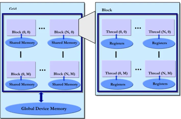
Thread (N, M)Figure 1: The CUDA grid and block structure.
in a thread block and the number of thread blocks within a grid. Figure 1 describes the CUDA grid and block structure graphically.
The graphics processor consists of multiple cores called tiprocessors, that can execute SIMD-instructions. Each mul-tiprocessor has access to a processor local memory that can be accessed with speed comparable to accessing a register. This memory is known in CUDA terminology as the shared memory as shown in Figure 1. A thread block consists of a specific number of threads, and is assigned to a specific mul-tiprocessor until it has finished its task. The threads in the thread block works together to perform SIMD-instructions and can communicate with each other using the shared mem-ory together with the hardware thread-barrier function sync-threads. This function acts as a synchronization point, caus-ing threads to wait at this point until all of the threads in the thread block have reached there. All multiprocessors ac-cess a large global device memory that is relatively slow as it does not provide caching.
The allocation of the number of thread blocks to each mul-tiprocessor is dependent on the amount of shared memory and the number of registers required by each thread block. More memory and registers required by each thread block means allocation of less thread blocks to each multiproces-sor. In this case the remaining thread blocks have to wait for their turn for execution.
3.
IMPLEMENTATIONS
A* is a standard path finding algorithm used to find the shortest path between two nodes in a graph. The classic representation of the A* algorithm is f (x) = g(x) + h(x), where g(x) is the total cost of the path to reach the current node x from the start node, and h(x) is the estimated cost of the path from the current node x to the goal node. f (x) is the distance-plus-cost heuristic function (or simply F-cost). This heuristic function is said to be admissible if the cost of the path estimated by it never exceeds the lowest-cost path. Since h(x) is part of f (x), the A* algorithm is guar-anteed to give the shortest path, if one exists. We are using the manhattan distance to estimate h(x) because manhattan distance works better on the squared grid maps that we use in our experimentation [5]. The manhattan distance is the
direct distance from current node to the goal node without considering obstacles in the path, hence it always calculates the shortest possible distance.
3.1
Standard A*
We are considering the map (search space) as a uniform two-dimensional grid that is subdivided into small square shaped walkable and non-walkable tiles. The algorithm searches only walkable tiles of the map; non-walkable tiles are sim-ply ignored. Figure 2 demonstrates the search space; Green is start node; Red is goal node; Gray represents unwalk-able nodes. Agents can move to adjacent tiles (eight ad-jacent tiles in our case); including diagonals. The cost to move straight horizontally or vertically is 10 and the diago-nal movement cost is set to 14 (√102+ 102). The A* search
algorithm finds the optimal path using the F-cost value of nodes. The nodes with the lowest F-cost values are remem-bered and searched first. The nodes that have already been visited are also remembered, so that they are not checked repeatedly. In this way each node gets one of the following statuses, ’not visited’, ’open’, or ’closed’. The node that has status ’open’ is placed on a list called the open list. An optimized way to maintain this sorted list is the use of a priority queue [4], like the one by Sundell et al. [13]. When all neighbor nodes of an open node have been visited, its status is changed to ’closed’ and this node is removed from the open list. The open list array is sorted using binary heap sort according to the F-cost values.
Figure 1: Arrows are pointing towards parent nodes; final path is represented using cyan arrows.
Figure 2: Standard A* algorithm search area. The algorithm starts when the current node (start node at the beginning) is placed on the open list. Then its eight adjacent neighbor nodes are visited and are put on the open list, their status becomes open, their G-cost, H-cost, and F-cost values are computed and G-cost and F-cost values are stored. The current node’s id is stored and marked as the parent of these neighbor nodes. The current node is done at this stage and its status is changed to closed, and it is removed from the open list. In the next step, these neighbor nodes become parent nodes of other visited nodes, and so on. In Figure 2 the blue nodes represent the total space searched to find the optimal path. At the end of the search, if the path is found, the optimal path is retrieved by moving backwards from the parent of target node towards the start node. In Figure 2 the arrows are pointing towards parent nodes and the final path is represented using cyan arrows. This optimal path is stored in the path array. More
details and pseudocode is given in [9].
3.2
Pre-Calculated Paths
The algorithm runs in two phases. In the first phase, which is done off-line, it computes a set of paths and stores them. On a n × m map, the paths that are selected are the n paths that go from the top of the map to the bottom, and the m paths that go from the left to the right side of the map. In the second phase, all agents run concurrently and tries to find their respective paths with the help of these pre-computed paths. When a new agent starts to find a path, it first checks in the list of pre-computed paths whether this path has already been computed and stored. If yes, then the search is stopped and the path is simply copied. If no, then the agent will check if there are partially pre-computed paths. In the case no pre-computed paths are matched fully or partially, the new path is computed from scratch.
3.3
Multiple threads per Agent
To allow for the A* algorithm to have multiple threads helping the same agent, some improvements where required to the basic algorithm. When many threads access the same shared memory, thread synchronization becomes es-sential for correct execution of the algorithm. We are using eight threads in parallel to work concurrently instead of one thread working in a loop. Eight threads are used because the grid illustration is used for the map representation in which each node has maximum eight neighbors. A data struc-ture called a ’temporary list’ is placed on the CUDA shared memory and is used by the eight threads in the thread block. It has an array with eight positions; one position for each thread. When each thread has evaluated the F-cost of its assigned neighboring node, it is stored in the list. Then all the threads are synchronized using the thread barrier func-tion. After this step only one thread runs for the remaining portion of the algorithm and the new nodes are placed on the open list with their correct F-cost. The pseudocode is given in [9].
3.4
Hierarchical Breakdown
For large graphs, the memory requirements of the algorithm increases, which results in fewer thread groups running in parallel on CUDA architecture and more time is required to find the paths. Therefore, to find paths on larger graphs, we have implemented a hierarchical breakdown scheme of A* (HBDnA*) using path abstraction and a refinement tech-nique. The idea is to find paths in small parts or slices and then put those path slices together. The search space is divided into smaller portions called clusters. Instead of applying a search on the whole graph, the search is applied on smaller clusters of the graph, hence lowering the memory requirements and fulfilling the memory limitations of un-derlying graphics card and CUDA architecture. The whole process of path finding is then done in the two steps: Path Abstraction and Path Calculation.
Path Abstraction
Path Abstraction also called path slicing, is a one time ac-tivity in which an abstract weighted graph is made from a grid map representation. The whole grid map is divided into clusters, which are connected to each other at specific points on the borders of the clusters called the exit points.
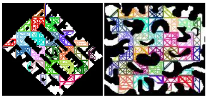
Figure 3: Abstract weighted graph for map A and B using cluster size 20 × 20.
Inter-edges (adjacent exit points of different clusters that are connected) and intra-edges (exit points that are connected to each other within the clusters) are computed to make an abstract weighted graph. An adjacency list is used to implement the graph. This graph is stored in memory and all further path finding is done at a higher level of abstrac-tion, using this weighted graph. Figure 3 shows the abstract weighted graph for cluster size 20×20 for two different maps used to take results.
Path Calculation
All the actual paths are computed after the path abstraction phase. This is done in the following three steps: In the first step all the start and target nodes are added to the abstract weighted graph by connecting each start and target point to all exit points of their respective clusters. Then the complete abstract paths are computed on the abstract weighted graph at a higher abstraction level instead of actual map. Paths found at this higher level are optimal and small and do not include low-level path details. They only include the high level moves, i.e. moving from one cluster to another cluster until target node is reached without considering low-level detailed paths within the clusters. The abstract weighted graph is much smaller in size as compared to the actual map size, therefore; the search is fast. Further the smaller size of abstract weighted graph also overcomes the memory lim-itations of GPU architecture. The third step is called path refinement and in this step all the abstract paths are refined to low level paths. Already searched and stored detailed paths are patched up to abstract path to give a complete path. Figure 4 visualizes 1000 complete paths for the two different maps used to take the results. The implementation details of path abstraction and calculation are given in [9].
Figure 4: Complete paths for 1000 agents for map A and B.
Our technique is similar to the hierarchical path-finding in [2], where the technique is implemented on a single proces-sor and the clusters are connected using eight exit points. We have used twelve exit points. As a consequence, the ab-stract weighted graph contains a greater number of nodes compared to the technique in [2]; this helps in increasing the path optimality.
4.
EXPERIMENTAL EVALUATION
The graphics processor used to run the experiments was a NVIDIA’s GeForce GTX 260 with 24 multi-processors; each multiprocessor contains 8 processor cores, so it becomes a total of 192 processor cores. It has a 576 MHz graphics clock, 1242 MHz processor clock, 896 MB standard memory, and a 36.9 (billion/sec) texture fill rate.
Map Size Walkable Nodes Agents
M0 3 × 3 8 64
M1 6 × 6 32 1024
M2 9 × 9 64 4096
M3 13 × 13 129 16641
M4 17 × 17 245 60025
Table 1: Benchmarks for standard A*, pre-calculated paths and multiple threads per agent. The experimental results for the standard A*, pre-calculated paths and multiple threads per agent implementations have been acquired using the same benchmarks used by Bleiweiss [1] and are presented in Table 1. In these benchmarks we measure the time it takes to calculate the path from each walkable node to all other walkable nodes. The number of agents are thus the square of the number of walkable nodes. From the results shown in Figure 5, it is obvious that pre-calculated paths and multiple threads implementation are much faster than the standard A* implementation for GPUs.
7000 0 5 10 15 20 25 30 35 M0 M1 M2 M3 M4 T im e /A ge nt (µs ) Standard A* Pre-Calculated Paths Multiple Threads
Figure 5: Standard A* compared to A* with pre-calculated paths and multiple threads.
Pre-calculated paths implementation gives the most efficient results because all the paths are not computed fully or par-tially. The implementation of multiple threads per agent takes less time than standard A*, but a little more when compared to pre-calculated path due to the binary heap that becomes the bottleneck. Eight threads run in parallel per agent, but when it comes to place the values in the binary heap, only one thread remains active and all the other seven threads wait.
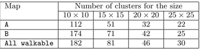
Map Number of clusters for the size 10 × 10 15 × 15 20 × 20 25 × 25
A 112 51 32 22
B 174 71 42 25
All walkable 182 81 46 30
Table 2: Number of clusters for different cluster sizes.
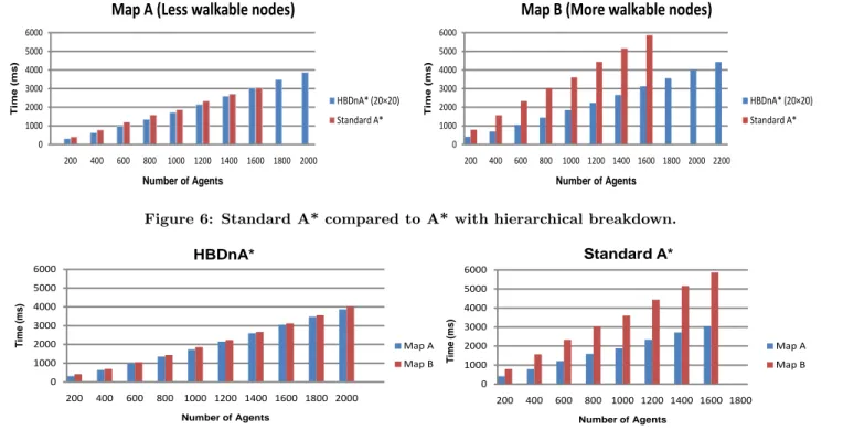
The maps used to take results for standard A*, Pre-calculate paths and Multiple Threads are very small in size, therefore, not very practical. For bigger sized maps, the memory limi-tations of GPU architecture is an obstacle. HBDnA* is used to find paths on bigger sized maps. The results for HBDnA* are based on two different maps (both sized 140×130 nodes), where map A has less walkable area compared to map B. A map with no obstacle is used in a few experiments to check the effect this has on the efficiency of HBDnA*. Figure 3 shows the abstract weighted graph for cluster size 20×20 for both maps, and Figure 4 visualizes 1000 calculated paths. The results from running standard A* and HBDnA* on both maps are shown in Figure 6. For map A both implementa-tions show approximately the same results, except that the standard A* can not handle more than 1600 agents due to its high memory requirements. For map B the results re-veal a drastic change in the behavior of the standard A* algorithm. It not only stops at 1600 agents, but also takes much more time to calculate the paths for fewer number of agents than HBDnA*. We can see that HBDnA* show a very steady and consistent result, even when the walkable area increases (map B), compared to the standard A* that shows a big increase in the path calculation cost with the increase of walkable area.
Figure 7 shows a comparison of the results of HBDnA* (clus-ter size 20×20) with standard A* on map A and B. HBDnA* implementation provides more consistent and stable results for both the maps and is not affected by the increase in the walkable area. Hence it is good for calculating paths on big images or images with more walkable or white space. While Standard A* implementation provides irregular and change-able results for both the maps and when the walkchange-able area increases (map B), the time for path calculation increases and at 1600 agents it becomes almost double as compared to time of map A.
To decided upon a suitable cluster size for HBDnA*, we have performed experiments using different cluster sizes on three different maps. The cluster sizes used are 10 × 10, 15 × 15, 20 × 20, and 25 × 25. The total number of clusters for these cluster sizes on the three maps (map A, map B, and all walkable map with no obstacle) are given in Table 2. Map A has less number of clusters because of less walkable area, as no clusters are required on unwalkable areas. Map B is divided in more clusters as compared to map A because it has more walkable area than map A. All walkable map (with no obstacle) is used to check the extreme values and to decide about the most appropriate cluster size; it is divided into the maximum possible number of clusters. Figure 8 presents the results of HBDnA* for the cluster sizes given
0 1000 2000 3000 4000 5000 6000 200 400 600 800 1000 1200 1400 1600 1800 2000 Tim e ( ms ) Number of Agents
Map A (Less walkable nodes)
HBDnA* (20×20) Standard A* 0 1000 2000 3000 4000 5000 6000 200 400 600 800 1000 1200 1400 1600 1800 2000 2200 Tim e ( ms ) Number of Agents
Map B (More walkable nodes)
HBDnA* (20×20) Standard A*
Figure 6: Standard A* compared to A* with hierarchical breakdown.
0 1000 2000 3000 4000 5000 6000 200 400 600 800 1000 1200 1400 1600 1800 2000 T ime (ms) Number of Agents HBDnA* Map A Map B 0 1000 2000 3000 4000 5000 6000 200 400 600 800 1000 1200 1400 1600 1800 T ime (ms) Number of Agents Standard A* Map A Map B
Figure 7: HBDnA* (cluster size 20 × 20) compared to Standard A*.
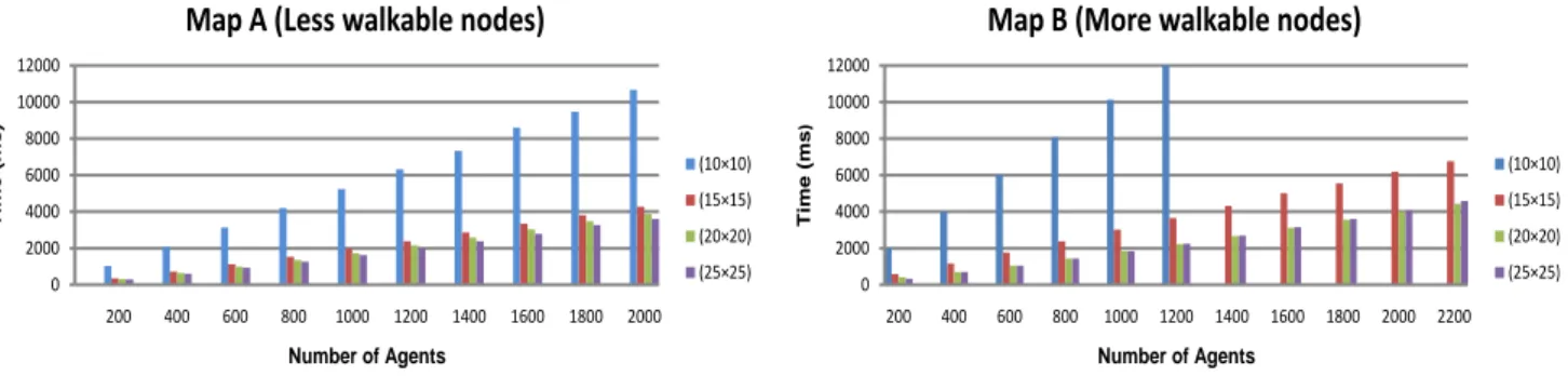
in Table 2 for the maps A and B. It is obvious from the results that the cluster size 10 × 10 takes much more time than the other cluster sizes for both map A and B because of the larger number of clusters. For map B it cannot run for more than 1200 agents which mean that with the increase in walkable area, the memory requirements for 10 × 10 cluster size increases rapidly and execution of more than 1200 agents becomes impossible.
Smaller cluster sizes leads to a larger number of clusters, which increases the GPU memory requirements and there-fore, reduces the number of agents that can run concurrently. A path calculated on the abstract graph is always optimal, but the path at the lower level of the hierarchy can be sub-optimal. The probability for sub-optimality increases as the size of the cluster increases.
The efficiency of the HBDnA* implementation is therefore a tradeoff between speed and optimality. The sub-optimality increases with the increase in cluster size. While decreasing the cluster size, increases the time to calculate the path. We want to calculate a path that is close to the optimal path and takes as little time as possible to calculate. Examining the results of Figure 8, we can see that the cluster size 20 × 20 shows the best tradeoff. It takes less time to calculate paths with this cluster size than with cluster sizes of 10 × 10 or 15 × 15, and we get paths that are closer to the optimal than with a cluster size of 25 × 25. Figure 9 presents the results of HBDnA* for the cluster size 20×20 for all the three maps. It is obvious that the results are stable and even for increased walkable area (like for map B and all walkable map) the results are regular.
The abstract weighted graph calculation is a one time
ac-tivity that is performed at the start of the HBDnA*. The total amount of time to calculate the abstract paths for all the three maps using different cluster sizes is presented in Figure 10. It indicates that it takes much shorter time to calculate the abstract paths. Further different cluster sizes do not affect the time required to calculate the abstract path by much.
5.
CONCLUSIONS
The memory requirements for the standard A* algorithm grows quickly as the size of the map increases. This leads to fewer number of thread blocks that can run concurrently on the CUDA architecture and thus decreases the speed of the algorithm. We have implemented three improvements to the standard A* algorithm on a graphics processor to increase performance and to allow it to calculate paths for a greater number of concurrent agents.
We have shown that our pre-calculated path and multi-ple thread immulti-plementations give good results for smaller maps. In the pre-calculated paths implementation we have pre-computed some paths and then shared these calculated paths during run time with other agents. This reduces the calculated cost of already computed paths. In the multiple threads implementations we have made some improvements to the standard A* algorithm to allow it to calculate each path using multiple threads that run concurrently and use shared memory and thread synchronization for communica-tion. It reduced the total search time as compared to the standard A* implementation.
The HBDnA* implementation shows faster and more consis-tent results for larger maps. To overcome the high memory needs for the larger maps, the search space is divided into
0 2000 4000 6000 8000 10000 12000 200 400 600 800 1000 1200 1400 1600 1800 2000 Tim e ( ms ) Number of Agents
Map A (Less walkable nodes)
(10×10) (15×15) (20×20) (25×25) 0 2000 4000 6000 8000 10000 12000 200 400 600 800 1000 1200 1400 1600 1800 2000 2200 Tim e ( ms ) Number of Agents
Map B (More walkable nodes)
(10×10) (15×15) (20×20) (25×25)
Figure 8: Results of HBDnA* for different cluster sizes.
0 1000 2000 3000 4000 5000 6000 200 400 600 800 1000 1200 1400 1600 1800 2000 T ime (ms) Number of Agents Map A Map B All Walkable
Figure 9: HBDnA* for cluster size 20 × 20 for map A, B, and All walkable.
0 200 400 600 800 1000 1200 1400
Image 1 Image 2 white
T ime (ms) 10*10 15*15 20*20 25*25
Figure 10: Time to calculate abstract weighted graph.
smaller areas called clusters; an abstract weighted graph is made that connects these clusters. Then multiple paths are computed on this abstract weighted graph which is much smaller in size than the original map. And finally, the com-plete paths are found using path refinements. The abstract weighted graph calculation is a one time activity and takes very little time. Our results have shown that the most appro-priate cluster size using HBDnA* for the graphics processors is 20 × 20.
Acknowledgments
This work was partially supported by the EU as part of FP7 Project PEPPHER (www.peppher.eu) under grant 248481 and by the Swedish Research Council under grant number 37252706. Daniel Cederman was supported by Microsoft
Re-search through its European PhD Scholarship Programme.
6.
REFERENCES
[1] A. Bleiweiss. GPU Accelerated Pathfinding. In Proceedings of Graphics Hardware, pages 65–74, 2008. [2] A. Botea, M. Muller, and J. Schaeffer. Near optimal
hierarchical path-finding. Journal of Game Development, 1(1):7–28, 2004.
[3] V. Bulitko, N. Sturtevant, J. Lu, and T. Yau. Graph abstraction in real-time heuristic search. Journal of Artificial Intelligence, 30:51–100, 2007.
[4] T. Cazenave. Optimizations of data structures, heuristics, and algorithms for path-finding on maps. In IEEE Computational Intelligence and Games, 2006. [5] R. Dechter and J. Pearl. Generalized best-first search
strategies and the optimality of A*. Journal of The ACM, 32(3):505–536, 1985.
[6] D. Harabor and A. Botea. Hierarchical path planning for multi-size agents in heterogeneous environments. In IEEE Symposium on CIG, 2008.
[7] P. Hart, N.J.Nilsson, and B. Raphael. A formal basis for the heuristic determination of minimum cost paths. IEEE Transactions on System Science and Cybemetics, 4:100–107, 1968.
[8] R. Holte, T. Mkadmi, R. Zimmer, and A. MacDonald. Speeding up problem-solving by abstraction: A graph oriented approach. Artificial Intelligence Journal, 85(1-2):321–361, 1996.
[9] R. Inam. A* Algorithm for Multicore Graphics Processors. In Master thesis, Chalmers University of Technology, 2010.
[10] R. E. Korf. Depth first iterative deeping: An optimal admissible tree search. Journal of AI, 1985.
[11] R. E. Korf. Real-time heuristic search. Journal of Artificial Intelligence, 42(2-3):189–211, 1990.
[12] N. Sturtevant and M. Buro. Partial pathfinding using map abstraction and refinement. In AAAI, 2005. [13] H. Sundell and P. Tsigas. Fast and lock-free
concurrent priority queues for multi-thread systems. JPDC, 65(5):609 – 627, 2005.