The Impact of Immigration on Income Inequality : Evidence from Sweden and the United States

(1)

School of Business, Society and Engineering Bachelor Thesis in Economics

Mälardalens Högskola Spring 2019

The Impact of Immigration on Income Inequality

Evidence from Sweden and the United States

Castoe, Minna Sanyal, Aalekhya

Supervisor: Johan Lindén Examiner: Christos Papahristodoulou

(2)

ii

Acknowledgments

We would like to acknowledge all those who have helped us complete this thesis, without whom this would not have been possible. Primarily, we would extend our thanks and gratitude to our supervisor, Johan Lindén,

who supported us through the entire process of producing this work. We would also like to extend a special thanks to Erick Mokaya, who

(3)

iii

Abstract

This paper studies data from a 25-year period in the history of Sweden and the US, ranging from 1993 to 2017. The aim of the thesis was to investigate the impact of immigration on the income inequality of the respective countries while also considering the impact of other specific variables. In order to estimate the impact of the variables, both static and dynamic models were used, with the Gini coefficient being the dependent variable. With the ordinary least square giving short-run estimates and the error correction model providing short- and long- run estimates simultaneously, the main variable for immigration, being the foreign-born population, showed a strong positive relationship with income inequality. For the estimation, the immigration variable was also split into high- and low-skilled immigrants as well as different age groups. In conclusion, we find that immigration in Sweden and the US has high levels of influence on the income inequality for both countries.

(4)

iv

1. Introduction

1.1 Problem

Social integration within the economy is becoming increasingly prevalent with the development of society. With this growth of society, diversity among groups of people continues to become more apparent with more people migrating from country to country each day. While migration works in both ways, certain countries face far larger extents of immigration due to unforeseen circumstances, leading to massive influxes of foreign population. The impact that immigration has on a country’s economy is largely varied and dependent on the type of immigration. There is however a consensus that large proportions of immigration impact the income distribution in society and thereby has an effect on a country’s income inequality, both in the short-run and the long-run.

Over their respective historical timelines, Sweden and the US have faced periods of

increased immigration as the direct or indirect result of several global events. These periods of immigration, whether due to labor, conflict, etc. have had significant impact on the respective economies of both countries and in accordance with the previously stated consensus, there has been impact on their respective income inequalities.

1.2 Aim

Based on a timeline of the 25 years, the study aims to empirically measure how significant the immigration has been in terms of impacting income inequality, while simultaneously taking into consideration several other variables such as, unemployment, trade, government distribution, etc. As a part of the study, the thesis aims to compare the inequality of income of the two countries in terms of both short-run and long-run as the effect of immigration, among other variables, may have varying degrees of impact on income inequality over extended periods of time.

1.3 Methodology and data

In order to complete the empirical study as successfully as possible, multiple regressions are be conducted for both countries, using the Gini coefficient as the primary measure of income inequality. The general structure for the method will be similar to a previous study

(6)

2 done upon the topic of Immigration and income inequality in the American States by the University of the Rhode Island faculty. In said study, the effects of immigration had been analyzed over a period of 15 years, using methods such as OLS to measure the short- run impact, complemented by a dynamic model known as the Error correction model (ECM) which measures the impact over the short- and long- run (Xu, P., Garand, J. C., & Zhu, L., 2016).

As mentioned, a similar approach is taken in this thesis with usage of both the OLS and Error correction model serving the same purpose as the previous study, providing estimations of the long- and short- run effects of immigration on income inequality.

The process is initiated by using OLS in a regression that provides fundamental insight into the relationship that immigration and inequality of income has. For this

regression, the Gini coefficient is used as the dependent variable with the independent variable being foreign-born population, representing immigration. Following this, are regressions where the foreign-born population is the developed and split into two main groups. The two groups that the immigration variable is split into are: low-skill and high-skill immigrants. Having two such groups avoids the potential situation where the variable is too generalized thereby, giving more comprehensive estimations. Each variable that has had data collected for is put into regression models and estimated using OLS. It is to be noted that because this is a comparative study, each regression is done for Sweden and the US respectively. Using OLS as the estimator provides estimates for static time series data, which shows the impact that immigration has on income inequality in the year of which the data is collected. The one-year period is what is being considered the short-run (Xu, P., Garand, J. C., & Zhu, L., 2016).

The data that the study is based on is multiple time series data and the

dependent variable, being the Gini coefficient, has a long-run stochastic trend. The nature of this variable implies that the impact which the independent variables from the times series data may have on the dependent variable would not entirely or necessarily appear in the year from which the data is collected. Consequently, this means that if there is a change to an independent variable at a time ‘t’, the effect on the dependent variable may be

(7)

3 mean that if there is an influx of immigration in one year, the effects on income inequality is likely to be evident in following years.

In order to gauge this, the dynamic multiple time series model, the Error correction model, is used to understand the impact that the independent variables have on the income

inequality in the long- run and the short- run.

1.3.1 Ordinary Least Squares (OLS)

Ordinary least squares (OLS) is an estimation technique that is used in linear regression models. One of the fundamental purposes of using OLS is that the estimates that it provides minimizes the sum of squared residuals in the β estimates which consequently minimizes the variance (Studenmund, 2017).

To be most efficient in the usage of this estimator there are seven classical assumptions that should be considered when making the regression model. When followed, as implied by the Gauss-Markov theorem, OLS is the “Best Linear Unbiased Estimator” or BLUE, where the “Best” implies minimum variance on the β estimates (Studenmund, 2017).

1.3.2 Error correction model

The Error correction model is a dynamic multiple time series model that is used when the variables, based on the data, have long-run stochastic trends or are cointegrated. This method is useful when estimating the short-run and long-run effects of data from one time series on data from another time series.

The essence of using this method is a multi-step process that begins with initially checking the time series data to ensure that it is in fact non-stationary. This leads to a modeled equation that is then estimated using the OLS technique (Xu, P., Garand, J. C., & Zhu, L., 2016).

1.4 Limitations

A primary limitation for this study is based on the accumulation of data. As the information required to conduct an entirely comprehensive study on this topic requires complete coverage of time series data over a 25-year period of time, there is dependency on the availability of such data.

(8)

4 As this thesis is an empirical study using econometric methods and multiple time series data, the basic problems that can be encountered when conducting such a study are potential limitations in this case too. With emphasis on the time series data, an expected limitation is the existence of serial correlation. This implies that there may be correlation between the error terms of observations from different time periods. Despite expecting this limitation, it proved not to be a problem for successfully conducting the study.

In terms of further limitation with time series data is the number of observations which are being used to run regressions. If the number of observations is too small, the significance of certain variables may be hampered (Studenmund, 2017).

(9)

5

2. Background - Immigration and inequality in Sweden and US

2.1 Focus on Sweden and US

The thesis studies the comparative impact of immigration on income inequality between Sweden and the US. Regarding the selection of the subject nations, there are several factors that have promoted the decision.

Sweden, despite its relatively small size, has been largely subjected to several periods in history that have shown large influxes of immigrants into the country for varying reasons and magnitudes. The most recent of these heavy immigration periods has been the immigration crisis of 2015. During this time, following the war that began in Syria in 2013, refugees migrated to Sweden in record breaking numbers. The years that followed

drastically increased the net foreign-born population in the countries and among other societal events, gave rise to the Swedish Nationalist political party called “Sverige

Demokraterna”. The impact that this immigration has had on the Swedish society is evident in the way immigration is publicly perceived, making the topic relevant in terms of current events (Roden, 2018). Along with the strict tax and government distribution laws that Sweden harbors, studying immigration’s impact on the inequality of income, appeared an interesting subject.

The economic system of capitalism has, historically, been very relevant in the US, prompting income distributions to become continuously skewed, with the wealth distribution in the US, in 2016, showing that the top 1% of the country owned a 38.6% share of the whole country’s wealth (Suisse, 2016). Relevant to the wealth distribution,

historically, US has had significantly higher Gini coefficient values than countries which are relatively similar in economic status, making the topic of income inequality a fascinating topic of study.

In terms of the immigration, as of January 2017, when Donald Trump was elected as the president of the US, controversial opinions and laws regarding immigration in the US have been passed (Sweet, D., 2017). These significant, while not necessarily desirable, shifts in societal stature gives rise to possibilities in understanding the state of the US

economy from the perspective of those who have political influence in the country as well as inhabiting consumers.

(10)

6 2.2 Types of Immigration

By definition, immigration is travelling to another country with the purpose of permanent residency there, with the hope of having a better life (USC 1101, 2019). While this is essentially true for all immigrants, the reason for migrating from one’s countries, is often significantly different. This in turn leads to there being differing types of immigration. The relevance of this to the thesis is that it is often observed that different types of immigration have impacts on different parts of a country’s economy as well as there being different degrees of impact.

A refugee is a status that given to any person outside their country of habitual residence that cannot or is unwilling to go back due persecution or fear of persecution (USC 1101, 2019). This is often an occurrence that happens when there is conflict in a person’s homeland and in order to escape it, migrates to another country, without necessarily having the legal documents.

There is a type of immigration that is based on finding work in a country outside the individual’s country of habitual residence. This is known as Economic

immigration or Labor immigration. It is quite common to find this among those who move from countries of lower economic status to one of higher status with the hopes that the work the person does in their homeland will generate increased income if done in the foreign country.

2.3 Comparison of historical Immigration

Throughout Swedish history, immigration has been an integral part of the society. Since World War II ended in the mid -20th Century, Sweden has been a host to those seeking residence and refuge in order to reestablish a peaceful life. A large part of this immigration was in fact, categorically, labor immigration with the most evident examples of people being large groups of Finnish, Italian, Greek, Turkish, Balkan and former Yugoslavic migrants who came to Sweden during the period of time, lasting until the late 1970s (Sweden and

migration., 2017).

From the early 1980s to the early 2000s is period in Swedish history that is classed as the beginning of Asylum seekers or refugee immigration. This was largely due to the two wars that happened in Iran-Iraq, in the late 1970s, and the wars in former

(11)

7 Yugoslavia. As a result, thousands migrated to Sweden seeking refuge and a substantial increase in net immigration was apparent (Sweden and migration, 2017).

Following the start of the war in Syria in 2013, further hundreds of thousands of refugees migrated to Sweden and in 2016 recorded a total of 162,877 asylum seekers (SCB, 2016).

The history of immigration to the US has similarities with that of the Sweden’s immigration history in the sense that it features different types of immigration in different periods of the historical timeline.

During the events of World War II, there was a lack of workforce in the US and consequently, the Bracero program was introduced (Franky Abbott, Hillary Brady, 2015). This program allowed Mexican agricultural workers to migration the US for contracted periods of time with a designated minimum wage. This is an example of one of the largest labor

immigration periods in the US (USfact, 2019).

After the conclusion of the war, several hundred thousand refugees were taken in by the US over a period that has continued into the modern-day US. Largely because the refugee immigration has been happening in such a large magnitude, over the past the 40 years, several political acts have been placed which have increased the US’ capability to take in refugee while also attempting to reduce the population of illegal immigrants in the

country (Sweet D., 2017; USfact, 2019).

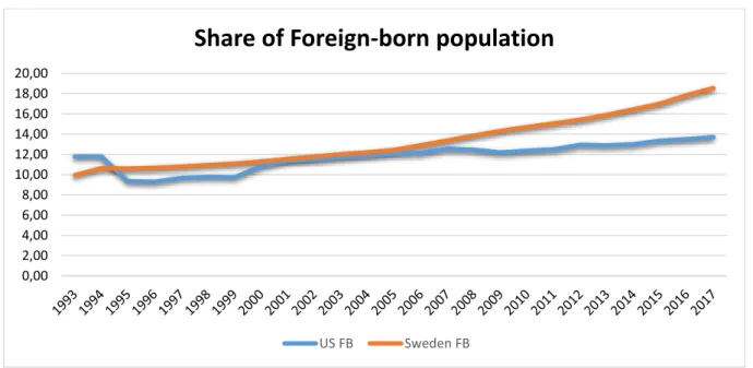
Figure 1.1 – Graph showing the total percentage of respective populations in Sweden and the US (add source)

Source: Author, Data are from Statistics Sweden (SCB) from 1993-2017 for Sweden. Current Population Surveys-Census Bureau for US.

0,00 2,00 4,00 6,00 8,00 10,00 12,00 14,00 16,00 18,00 20,00

Share of Foreign-born population

(12)

8 2.4 Cause of inequality of income

Inequality of income in a country is dictated by a large variety of economic factors. A paper published by Dabla-Norris, M. E., Kochhar, M. K., Suphaphiphat, M. N., Ricka, M. F., & Tsounta, E. (2015) describes the causes of income inequality in terms of drivers, with some primary drivers being based on global trade, financial depth, redistributive policies,

education, technology, immigration, etc.

Using technology as a driver for inequality in this case is considered in terms of a rising technological premium (Dabla-Norris, M. E., Kochhar, M. K., Suphaphiphat, M. N., Ricka, M. F., & Tsounta, E., 2015). The implication of this variable is that as technology develops, the ability to use the technology is the main consideration when defining the variable. Technological skill premium is the metric that measures the technically prowess of members in a population. This is similar to the education variable which is described by the paper as possibly having a positive or negative correlation with income inequality. The determinant of the variable’s correlation in this case, is the “rate of return” (Dabla-Norris, M. E., Kochhar, M. K., Suphaphiphat, M. N., Ricka, M. F., & Tsounta, E., 2015) that the education of an individual has.

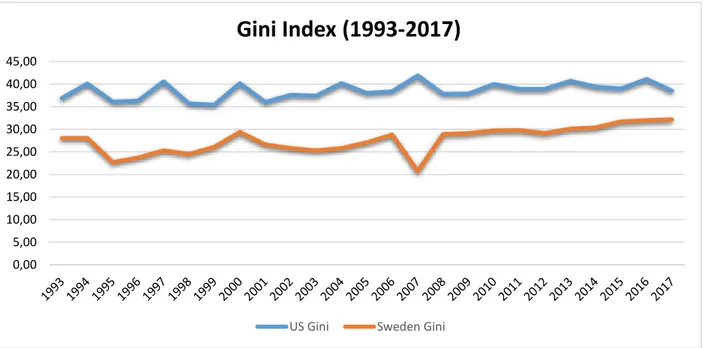
Figure 1.2 – Graph showing the Gini index trends in Sweden and the US

Source:Author, data are from the World Income Inequality Database (WIID)-United Nations University- World Institute for Development Economics Research (UNU-WIDER) for US. Sweden statistics (SCB) for Sweden.

0,00 5,00 10,00 15,00 20,00 25,00 30,00 35,00 40,00 45,00

Gini Index (1993-2017)

(13)

9 In a research article by Neckerman, Kathryn M, and Torche, Florencia (2007), income inequality is described with variables such as government policy changes, labor market fluctuations, age and skill-biased technical change, which is common to the research by Dabla-Norris, M. E., Kochhar, M. K., Suphaphiphat, M. N., Ricka, M. F., & Tsounta, E. (2015).

2.5 Gini Coefficient as a measure of inequality

The Gini coefficient is considered to be a primary measure of economic inequality, measuring how income is distributed in a population. In essence, the Gini coefficient measures the disparity between a perfectly equal population in terms of income and the actual income distribution. Numerically, this measure is derived from a metric displayed in a

Lorenz Curve (Borjas, 2016).

The Lorenz curve shows a measure of what share of income, different shares of households have in a population. As seen in figure 1.3, the Lorenz curve is presented

alongside a Line of Perfect-Equality that shows, as the name suggests, a population with a perfectly equal income distribution. By taking the ratio of the area between the Lorenz curve and the Perfect-equality line, against the entire area under the Perfect-equality curve, the number found, is the Gini coefficient (Borjas, 2016).

Figure 1.3 – A figure showing the income distribution with the Lorenz curve.

(14)

10

3. Literature review

The aim of reviewing existing literature and presenting them in this part is to predominantly justify the selection of variables and methods that have been used in this empirical study.

In the paper written by the Rhode Island research faculty (Xu, P., Garand, J. C., & Zhu, L. (2016)), the impact of immigration on income inequality is studied using static and dynamic models. The usage of static models aimed to provide an understanding of what the impact of immigration was on income inequality in a short- term, with OLS being the primary technique of estimation. It was theorized in the paper that the impact of the immigration would be more prevalently visible over the duration of a few years rather than just the year of immigration. To acquire an understanding of this, the Error correction model (ECM) was used to show how the income inequality was impacted in the long term.

The final consensus in the paper by Rhode Island research faculty (2016) was that immigration has a significant impact on the income inequality in the US however, the level of education that the migrating population had, was also of significance. While the Gini coefficient was used as a primary measure of income inequality, a different measure, namely income ratios, was used to see the impact on the immigration on the different parts of the wealth distribution, split into lower, middle and upper classes of society. Using the different models and the robustness tests of the income ratios, it is concluded that immigrants who are classed as low-skill immigrants provide a significant positive impact on the inequality of income while high skill immigrants manly reduce income inequality measures in the top decile of the population.

Concerning the inequality that arises from the immigration, is another study by E. Glen Weyl (2016) that looks upon the topic from a global and a domestic perspective. This paper discusses the ways in which migration is handled by the Gulf Cooperation Council (GCC) and how the OECD countries could see benefit from its methods. The consensus of the study implies that by the taking in larger numbers of migrants from relatively less wealthy nations, global inequality rates are reduced due the average utilitarian marginal value of a dollar when given to someone born outside the US. The study does however discuss that the increase in migration has a positive relationship with income inequality on a domestic level, further reinforcing the impact of immigration on income inequality.

(15)

11 On the basis of a study by Hainmueller, J., & Hiscox, M. (2010), there is clear division of how the public in the US views immigration. This further developed into

considering how immigrants of different levels of educational background are viewed. In this study, there the two main economic concerns regarding immigration with in most cases, low skilled immigration having a negative outlook. This is due to the economic concerns of there being more competition in the low skilled labor market and that public services would be burdened by the influx of this low skilled population. As this 2010 study depicts, division in the perspective is notably strong and thereby, for this thesis, the skill level of the immigrants is of significance.

Dale O. Collinger from the University of Houston-Clear lake outlines several factors that have significant influences on the Gini coefficient. His analysis, based on a statistical analysis of 53 countries, essentially divides the factors of the income inequality into, natural and policy dependent. Among the natural factors of income inequality is the variable of age (Collinger, 2016). The study indicates that the older part of the population shows lower values of the Gini coefficient than the relatively younger population. This is theoretically explained as the older population having diminished incentives to pursue higher incomes as retirement approaches.

As opposed to this, is a work by Mark Thoma (2015), which considers inequality of income, with age as the independent variable and explains that older households are more susceptible to income inequality than younger households. This is based on a rather philosophical argument on whether inequality is caused by ability or luck. With the variable being luck, Thoma (2015) suggests that as households grow older, external and unpredictable occurrences are determinants of income and eventually cause the income inequality of the older households to vary significantly.

Collinger (2016) outlines difficulties of natural causes of inequality and mentions that in order to work around these natural causes, long-term policy changes are needed to be made. Taxation is considered to be a variable that has a large impact on income inequality, where statistics in France and Switzerland suggest that the high marginal tax rates result in less inequality than for example the US (Collinger, 2016).

Gerald W. Schully (2008) considers taxation in a similar manner but in his work, he considers the relationship between tax rate, inequality and growth in terms of GDP. He

(16)

12 explains that nations with relatively high economic growth rates experience higher degrees of income inequality than countries with less growth. As the tax rate of 30.7 percent resulted in an average GDP growth rate of 3.4 percent per year, by using the Schully model (Schully, 2008), it showed that an optimal tax rate of 19.3 percent would give a growth rate 6.97 percent per year. Further developing the studies involving the tradeoff between taxation and the GDP per capita in the US, Schully showed that a 1 percent change in the GDP growth rate was associated with a 0.00075 change in the Gini coefficient assuming a derived optimal tax rate of 19.3 percent (Schully, 2008). In essence, this indicates a significant negative correlation between tax rates and income inequality, further reinforcing the work done by Collinger (2016).

Another study that strengthens the importance of tax, as well as, government distribution when assessing the income inequality, is a work by Anders Björklund (1998). In his study, Gini coefficients are found with the inclusion and exclusion of taxes and other government subsidies portrayed as disposable income. The results in the study show that with the inclusion of taxes and other government distributions, the Gini coefficient was significantly less in the Nordic countries, during the 1990s (Björklund, 1998).

The relationship between unemployment and income inequality is heavily theorized to have to strong positive correlations. Among works which support this theory, is that by Thurow (1987), who assess unemployment to have this positive relation with income inequality. The theory goes in accordance with the logical concept that when there is a large amount of unemployment in a population there is a significant decrease in income and therefore the population of the people in the lower income distributions of the population are greater (Thurow, 1987). This in turn, increases the value of the Gini coefficient.

Björklund (1991) published a work in the Scandinavian Journal of Economics that studied this relationship between unemployment and the income in during the period of 1970 – 1990. In this paper, despite having hypothesized that unemployment would logically cause income inequality due to there being a larger portion of the population with relatively little income, his results showed that there was no significant impact of inequality from unemployment. The paper then theorizes this to be result of the added worker effect, suggesting that when there is a case of unemployment in a household, members of that

(17)

13 household would work to make up for the loss of income. This theory was however later rejected in following studies.

A variable of notable importance for the estimation of income inequality in society is the measure of total investment. While the impact of the total investment on income inequality is subjective and thereby dependent on which country is being assessed, there are reoccurring trends which suggests a positive relationship between foreign direct investment (FDI) and income inequality, and since FDI increases total investment, a similar relationship is assumed. A paper by Macarena Suanes (2016) studies the relationship between the foreign direct investment and the income inequality in Latin American

countries and finds evidence that suggests a positive relationship between the two variables. A similar conclusion is found in a paper by NM Jensen and G Rosas (2007) that explains that foreign direct investment having a positive relationship with income inequality is largely due to a higher demand for high- skilled labor because of increased foreign

investment. This same paper does however outline that this conclusion may be less

applicable to less developed countries as in such situations, there is a difference in the type of FDI, possibly resulting in a decrease of income inequality with higher levels of FDI (Jensen, N. M., & Rosas, G., 2007).

An older study by Pan-Long, T (1995) from the National Tsing Hua University in Taiwan found, conversely to Jensen and Rosas (2007), that the income inequality in less developed countries is more positively related to foreign direct investment than was

hypothesized. In fact, the measures of income inequality in eastern Asian countries seemed to be less impacted by the variable than most other nations. These findings suggest foreign direct investment to have varying forms of impact on income equality but generally show a positive relationship.

Nielsen and Alderson (1997) studied income inequality in the United States between 1970 and 1990. In their studies, there was significant emphasis on different social groups in country, suggesting significant income disparity between people from the African-American population and the white population. Racial dualism indicators were used to measure this and it showed a significant degree of income inequality between the races (Nielsen and Alderson, 1997). From these results, conclusions were drawn that this variable is important when estimating inequality and therefore is considered in this thesis as well.

(18)

14

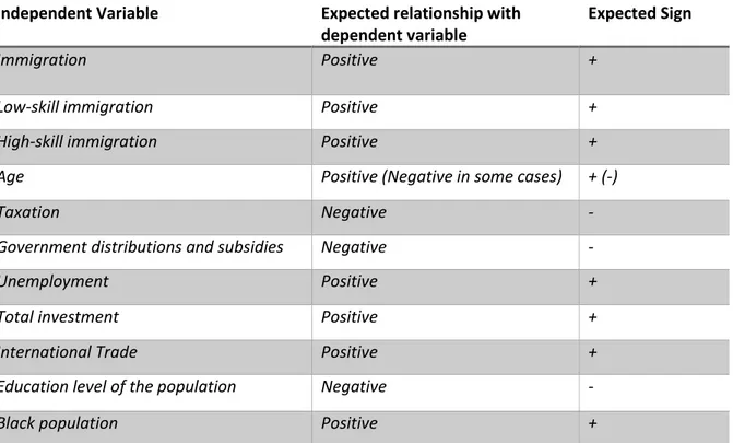
Independent Variable Expected relationship with dependent variable

Expected Sign

Immigration Positive + Low-skill immigration Positive + High-skill immigration Positive + Age Positive (Negative in some cases) + (-)

Taxation Negative -

Government distributions and subsidies Negative - Unemployment Positive + Total investment Positive + International Trade Positive + Education level of the population Negative - Black population Positive +

Table 1. Variables and Expected relationship with dependent variable

(19)

15

4. Empirical framework

4.1 Data

With the aim of exploring the impact of immigration on income inequality, we use multiple time-series data from Sweden and the US representing 25 years, from 1993-2017. We consider different groups of immigration to see which group has the strongest impact on income inequality according to age and educational attainment. In addition to immigration data, other sociodemographic variables are used in this paper as well as variables suggested by other researchers which have been known to influence the inequality of the income.

4.1.1 Dependent variable Income inequality

Income inequality among individuals can be measured by different indicators, with the Gini coefficient being one of its most extensively measures. According to The Organization for Economic Co-operation and Development (OECD), Gini Coefficient is used most widely to measure the inequality of the income, compared to other indicators. It measures an income which consists of earnings, self-employment and capital income as well as public cash

transfers based on the compression of cumulative proportions of population and cumulative proportions of their income. The Gini coefficient of a country ranges between 0 and 1, where a Gini coefficient of zero represents perfect equality and a Gini coefficient of 1 represents perfect inequality.

We use the Gini index as a measure of income inequality with it being our dependent variable in the regression models, where Gini index is the Gini coefficient expressed as a percentage between 0 and 100. Data for the measurement come from The World Income Inequality Database (WIID) provided by United Nations University- World Institute for Development Economics Research (UNU-WIDER) for US and from Sweden statistics (SCB) for Sweden.

(20)

16

4.1.2 Independent variables Immigration independent variables

For our immigration variables, first we consider the total number of all immigrants in a country as a share of the total population. Thereafter, we divide immigrants to different groups with different ages and different levels of education.

Foreign-born population

We use foreign- born population as a general measure of immigrants in a country. The measure includes anyone who is not a Swedish/US citizen at birth, with both permanent and temporary resident immigrants being included.

In this paper, we use the total number of foreign-born population in each of the two countries as a percentage of the total population. We expect that foreign-born population has a positive effect on income inequality, i.e. as the number of foreign-born population increases, Gini coefficient increases. Data on the measure come from Statistics Sweden from 1993-2017 for Sweden and from Current Population Surveys provided by Census Bureau for US for 1995-2016, where the average was included for the remaining years due to

unavailable data.

Age

Age is assumed to be one of the factors that influences income inequality. According to Thoma (2015), as people age; income inequality grows. This explains the median age of the population as having a significant impact on income inequality, which also was outlined in the statistical analysis by Cloninger (2016).

Rather than focusing on the median age of immigrants, which is supposed to have a significant impact on the income inequality, we consider two groups of immigrants where we include young immigrants and very old immigrants. For Sweden, we include a group of immigrants aged 16-25 and a group of immigrants aged 65-74 as a share of total foreign-born population. Whereas in the US, we include a group aged 21 and under, and a group aged 74 and older as a share of total immigrants. The aim of this is to see if any of these groups has a significant effect on income inequality. Data for the immigrants’ age

(21)

17 groups are acquired from Statistics Sweden for Sweden and from Current Population

Surveys, for the US.

Low-skill and high-skill immigration

We consider the educational attainment of the immigrants as a proxy for skill level.

Immigrants are divided into two groups according to the level of education they have, where each group represents the number of immigrants as a percentage of the total foreign-born population aged 16-74 for Sweden, and 25 years and older for US.

Low-skilled immigrants represents immigrants with no high school diploma and

high-skilled immigrants represents immigrants with post-secondary education or above.1_We

expect these two groups of immigrants to have a positive effect on income inequality. Data for the selected years also come from Statistics Sweden for Sweden and from Current Population Surveys for the US.

Total investment

The definition of total investment, also known as gross capital formation according to the World Bank, is the total value of the gross fixed formation and the net changes in the level of inventories. Suanes (2016) found that there is a positive relationship between foreign direct investment (FDI) and Gini coefficient, and since foreign direct investment increases the total investment and as a result, this is also expected to have a significant positive impact on income inequality.

Total investment is used as a measure of the investment of a country in terms of the total investment as a share of GDP. We expect that this variable has a positive effect on income inequality, i.e. higher investment leads to higher Gini coefficient. Data for this measure come from the World Bank for both Sweden and US from 1993-2017.

Tax Revenue

Cloninger (2016) has pointed out that taxation plays an important role in the estimation of income inequality. It is one of the variables which influences inequality of the income where

1 Post-secondary education in Sweden represents 3 years of higher education (after high school education), where it represents 4 years of higher education (undergraduate school) in US.

(22)

18 countries with high tax rate are assumed to have lower Gini coefficient compared to

countries with low tax rate. This may suggest a partial justification to the US having a higher Gini coefficient than Sweden where the tax revenue for the US ranges between 7 and 12 percent of the GDP and for Sweden it has reached approximately 30 percent of the GDP between 1993-2017.

Tax revenue is used as a measure of the overall tax in terms of revenue as a share of GDP, where tax revenue is the revenue which is collected from taxes on income and profits, taxes on goods and services, payroll taxes, social security contributions, etc. (The World Bank). We expect that tax revenue has a negative effect on income inequality, where higher tax revenue leads to lower income inequality.

Data on the measure are collected from The World Bank for both Sweden and US.

Subsidies and other transfers

Subsidies and other transfers as a share of the government expenses are also used in this paper to measure the amount of redistribution done by the respective governments. This measure provides an indication of the size of the government across the countries and it is also supposed to have a negative impact on income inequality since it involves redistribution of wealth. We include this variable in our US-model and Sweden-model and we expect that subsidies and other transfers have a negative effect on income inequality. Data for the US and Sweden, from 1993-2017, are acquired from The World Bank.

International openness indicator

International openness indicator is a common measure of international trade, it measures how open the country is for international trade. This indicator is a sum of both imports and exports within a country as a share of the GDP. The larger the ratio, the more the country is exposed to international trade.

We use international openness indicator as a variable for international trade, measured as a share of the GDP and we expect that has a positive effect on Gini coefficient, i.e. the more the country is exposed to international trade, the higher the Gini coefficient is. Also, we expect that trade is positively correlated with Gini coefficient because globalization

(23)

19 is a part of the international trade which is supposed to increase the income inequality. Data on the measure are collected from the World Bank for both countries.

Educational level-College graduates

Coady and Dizioli (2017) emphasize a negative relationship between the level of education of the population and income inequality. The educational level variable in this paper refers to the educational attainment of the total population who are college graduate, i.e. with at least three years of post-secondary education or more at age of 25 years and older for US, whereas the age is limited in Sweden between 25 and 74.

We use the number of people with post-secondary education as a share of total population as a measure for the educational level. We expect a negative relationship with income inequality since having a larger educated population reduces inequality of opportunity and thereby increases the average income (Coady and Dizioli, 2017). Data for the metric come from statistics Sweden (SCB) and the Current Population Surveys for Sweden and the US respectively.

Unemployment rate

Unemployment rate is a common measure of the unemployment in a country. To this

metric, the number of unemployed people are taken as a percentage of the total labor force. The unemployment rate is expected to have a positive effect on income inequality since higher unemployment rate leads to more people in the bottom of the income distribution. Data on the measure for 1993-2017 for both Sweden and US come from International Monetary Funds (IMF) which publishes a range of time series data provided by World Economic Outlook.

GDP per capita growth

GDP per capita growth refers to annual percentage growth rate of gross domestic product per capita. It is used in this paper as a measure of economic growth and development in a country. There is some debate about the relationship between the inequality of the income and the economic growth. Where some researchers have confirmed that the economic growth has a positive effect on income inequality, Cloninger (2016) finds that GDP per capita

(24)

20 has no measurable influence on income inequality when testing the impact of different variables on income inequality. To further examine this, we include this variable in our regression models and we expect that GDP per capita has a positive effect on income inequality. Data on the measure are from The World Bank from 1993-2017 for both Sweden and US.

Black population

Race is expected to influence income inequality in US where the share of black population is higher compared to Sweden. Statistically, the population of people with the “Black African descent” earn less on average than their white counterparts (Williams, 2011). Thus, we include this variable in our US-model expecting that black population has a significant positive effect on income inequality, where we use the number of black persons as a percentage of the total population. Data on the measure come from Current Population Surveys which is provided by Census Bureau.

4.2 Estimation Method

In order to investigate the impact of the immigration on income inequality, we use two different models. We consider the short-term effect as well as the long-term effect of different groups of immigrants on income inequality according to their age and their level of education.

For the short-run impact of immigration on income inequality, we estimate the full impact of foreign-born population on the income distribution using a proper static model which we estimate using the ordinary least square model (OLS). We use foreign-born

population as the only independent immigration variable to see the impact of the

immigration as a whole on income inequality and after that we include different groups of immigrants according to their age where we take a group of young immigrants (age 16-25) for Sweden and under age 21 for US. We also include another group of old immigrants, between the ages of 65-74 for Sweden and over 65 for US.

To estimate the long-run relationship between immigration and income inequality, we use a dynamic model. A dynamic model is a model where the lagged-term of

(25)

21 the dependent variable appears on the right-hand side of the equation together with the current value and the lagged-term of the independent variables.

Since our data is multiple time series data where our dependent variable Gini

index is supposed to have a long-run stochastic trend, thus, if there is a change in our

independent variables in time ‘t’, the full effect is not experienced in this period and it may take time for our dependent variable Gini index to adjust to the change in the independent variables at time ‘t’. To accommodate for this, we use a proper dynamic model to estimate the long- and the short-run impact of immigration simultaneously. The suggested model in this case is the error correction model (ECM). For this model, we estimate the change of our dependent variable Gini index as a function of the lagged-term of itself as well as the lagged- and first-order difference terms of all our independent variables.

As mentioned, different groupings of immigrants are considered for this model as well. First, we study the impact of immigration on income inequality as a whole and after that we divide the foreign-born population into two groups: low-skilled and high-skilled immigrants according to their level of education to consider which group has the highest impact on income inequality.

Furthermore, the order of observation is important to note when considering time-series data. Thus, analyzing time-series data requires some special care where one should take into account the trend of the variables as well as the stationarity. Therefore, before we start exploring the long- and short- relationship between immigration and income inequality using error correction model, it is strongly recommended that we test if our variables are stationary or not. That is done by either using a visual test where we plot our data and check if the properties are changing over time, or by using a statistical test where we test for unit roots using Dickey-Fuller test (DF), a widely used test for the stationarity of a variable. Stationarity is found after taking first difference of a variable, and a time series data which has a unit root is said to be nonstationary series, since the presence of the unit root leads to the violation of the assumption of constant mean and variance.

Stationary time series data is the data which has the basic properties of, either the mean or the variance being constant and not changing over time. In contrast, a

nonstationary series is a series which has its mean and/or variance being not constant with changes happening over time.

(26)

22 There are different types of stationarities, where time-series can be either strict stationary, trend stationary or difference stationary. A strict stationary series is the one with mean, variance and covariance not being a function of time. Whereas the trend

stationary and the difference stationary can be classified as nonstationary time series since the trend stationary series is a series with no unit root but exhibit a trend and once the trend is removed the series is said to be strict stationary series. KPSS

(Kwiatkowski-Phillips-Schmidt-Shin) test can be useful to remove the trend and make the series strict stationary. For the difference stationary however, Augmented Dickey –Fuller test can be used which is known as a difference stationarity test to make the difference stationary series strict stationary (Singh, 2018).

Moreover, once a time series is found to be nonstationary, it is important to make this series strict stationary in order to be able to estimate this series using different models. There are two well-known methods to convert the nonstationary series and make it stationary. The first method is “differencing” where we compute the difference of

consecutive terms in the series. It is typically performed to help stabilize the mean of the series. Another useful method is the “transformation” such as logarithms where

transformation is used to convert the nonstationary series into stationary series by stabilizing the non-constant variance of the series.

Another reason why it is important to test for the stationarity of the variables is to ensure that our regression results are not spurious. Spurious regression can also become an issue when analyzing time-series data, where time-series data which include both nonstationary dependent- and independent variables can cause that regression result to be spurious, i.e. spurious regression. To avoid this problem when working with time-series data, we test the stationarity of our variables and we also check that our results from estimating the short-run relationship between immigration and income inequality using ordinary least square are not spurious by using the Durbin-Watson Test.

Besides detection of spurious regression, the Durbin-Watson test is also used to test for serial correlation. In the accordance with the testing process, the Durbin-Watson statistics should be between 0 and 4 where Durbin-Watson statistics with a value of 2 implies that no autocorrelation is evident. A low Durbin-Watson statistic, which in such a case, is lower than the adjusted R square, implies that the regression result is spurious.

(27)

23 The following models are used for the empirical study:

4.2.1 Ordinary least square (OLS)

Ordinary least square regression is a generalized linear modeling technique that is used to estimate the linear relationship between two or more variables. With this knowledge, we start by exploring the short-term relationship between immigration and income inequality using OLS, where we assume that the factors are stationary for this static model, i.e. the mean and the variance are constant and do not change over time.

With the short-term relationship between immigration and income inequality being estimated by a static model, we estimate the following equation with OLS:

𝑦_𝑡= 𝛽₀+ 𝛽₁𝑥_𝑡+ 𝜀_𝑡 𝑤ℎ𝑒𝑟𝑒 𝑡 = 25 𝑦𝑒𝑎𝑟𝑠

4.2.2 The Dickey-Fuller Test

Using Dickey-Fuller test, we can determine if our variables are stationary or not, we can also ensure that our regression result is not spurious. However, there are three version of the Dickey-Fuller test which give the same results. We use the basic version with a constant term and no trend term included, and we estimate the following equation using ordinary least square:

𝑦_𝑡− 𝑦_𝑡−1= 𝛽₀+ 𝛽₁𝑦_𝑡−1+ 𝜀_𝑡

The null- and the alternate hypothesis of this test are:

Null hypothesis: 𝐻0 = The series has a unit root

Alternative hypothesis: 𝐻1= The series has no unit root

If the estimated beta (𝛽̂1) is significantly less than 0, then it is possible to reject the null

hypothesis of a unit root and conclude that the variable is stationary. Otherwise, the null hypothesis of a unit root cannot be rejected and thus this implies that the variable is nonstationary.

For this test, we limit our attention to test the stationarity of our dependent variable Gini

(28)

24

4.2.3 Autoregressive Distributed Lag model

The lagged-terms of the independent variables are used when analyzing time-series data whenever one expects that the independent variable affects the dependent variable after a period of time. Autoregressive Distributed Lag model however is a model used to deal with the time-series data. It includes the lagged-term of the dependent and independent

variables on the right-hand side of the equation. ADL model includes not only a one-time-period lag, but it includes also different-time-one-time-periods lag terms (one year, two years, etc.) of the dependent and independent variables. It explains the current value of the dependent variable as a function of current and past values of the independent variable and past values of the dependent variable as well. We use ADL (1, 1) model to derive the equation for the error correction model.

ADL (1, 1) is as follows:

𝑦_𝑡= 𝛼₀+ 𝛼₁𝑦_𝑡−1+ 𝛽₀𝑥_𝑡+ 𝛽₁𝑥_𝑡−1+ 𝜀_𝑡

4.2.4 Error correction model

With the time-series data that is being used, we need to study the short-term relationship as well as the long-term relationship between our dependent variable and independent

variables. A good time series model should consider both the short-run and the long- run equilibrium simultaneously and error correction model is used for this purpose.

The error correction model is the standard way to model time-series data since it captures both short- and long-term relationship between two variables. It separates the long- and the short- run relationship between two variables and make it possible to deal with nonstationary data series. There are two variants of error correction models, a one-step error correction model and a two-step error correction model (Engle and Granger,1987).

An assumption about the variables that is made when simultaneously exploring the short- and long- run relationship between immigration and income inequality using ECM, is that the variables are nonstationary.

A one-step ECM is used to estimate the dynamic model. This model consists of determining both short- and long-run relationship by estimating the first order difference of the dependent variable as a function of the one-time-period lag of the dependent and independent variables as well as the first order differenced independent variables where the lagged-term of the independent variables explains the long-run relationship, and the

(29)

first-25 order difference of the independent variables illustrates the short-run relationship between the dependent- and the independent variables.

One-step error correction model is determined as follows:

Consider the long-run equilibrium which is derived from autoregressive distributed lag (ADL) (1, 1), i.e. ADL includes a one-time-period lag of the dependent variable and one time-period lag of the independent variables on the right-hand side.

𝑦_𝑡= 𝛼₀+ 𝛼₁𝑦_𝑡−1+ 𝛽₀𝑥_𝑡+ 𝛽₁𝑥_𝑡−1+ 𝜀_𝑡

Assuming that 𝑥_𝑡 is stationary implies that 𝑦_𝑡 is also stationary. Thereby, given the

stationarity, the long-run equilibrium can be found:

𝑦_𝑡= 𝛼0

1 − 𝛼₁ +

𝛽0+ 𝛽1

1 − 𝛼₁ 𝑥𝑡+ 𝜀𝑡 Which can be written as follows

𝑦_𝑡¤ = 𝛾0+ 𝛾1𝑥𝑡+ 𝜀𝑡 (1) 𝑤ℎ𝑒𝑟𝑒 𝑡 = 25 𝑦𝑒𝑎𝑟𝑠, 𝛾0 = 𝛼0 1 − 𝛼1 𝑎𝑛𝑑 𝛾1 = 𝛽0+ 𝛽1 1 − 𝛼1 Adjusted equation: (𝑦𝑡− 𝑦𝑡−1) = 𝜆( 𝑦𝑡−1¤ − 𝑦𝑡−1) + 𝜙(𝑥𝑡− 𝑥𝑡−1) (2)

Substituting (1) into (2) gives

(𝑦𝑡− 𝑦𝑡−1) = 𝜆( 𝛾0+ 𝛾1𝑥𝑡−1+ 𝜀𝑡− 𝑦𝑡−1) + 𝜙(𝑥𝑡− 𝑥𝑡−1)

Long-run Short-run

Which gives: ∆𝑦_𝑡 = 𝜃₀+ 𝜃₁𝑥_𝑡−1+ 𝜌𝑦_𝑡−1+ 𝜏∆𝑥_𝑡+ 𝑣_𝑡

𝑤ℎ𝑒𝑟𝑒 𝜃₀ = 𝜆𝛾₀; 𝜃₁ = 𝜆𝛾₁; 𝜌 = −𝜆; 𝜏 = 𝜙; ; 𝑣_𝑡 = 𝜆𝜀_𝑡

The final equation represents the error correction model and can be estimated by using OLS. The lagged-term of the independent variable explains the long-run relationship between the dependent- and independent variables since it was derived from the long-run equilibrium equation, where the first order difference of the explanatory variable represents the short-run relationship between the dependent variable and the independent variables.

(30)

26

5. Empirical Results and Interpretation

Our results consist of two parts, the short- and the long- term effects of immigration on income inequality. Each part includes the estimation of the impact of immigration in Sweden as well as United states where different models are also included in each part. The first part is the estimation of the static model using OLS for the short-run relationship between immigration and income inequality. The second part is the estimation of the dynamic model using ECM for the long- and short-run relationship between immigration and inequality.

Using the data from 1993-2017, we focus our attention on the impact of immigration on income inequality using three significance levels, 1%, 5% and 10%. We also include other explanatory variables which are suggested by other researchers and which are expected to influence the income inequality.

In addition to this, we test the stationarity of the Gini index and our main immigration independent variable, i.e. foreign-born population using Dickey-Fuller test. We present the results of the test before we use the error correction model to estimate the short- and long-run relationship between immigration and income inequality to show that we have nonstationary variables.

5.1 Short-term effect of immigration on income inequality using OLS

As a starting point, we begin by estimating the short-run impact of immigration as a whole on income inequality for each of our two countries. We present the results in table 2 and table 3 with different models where we add and replace some of the explanatory variables.

5.1.1 Sweden

To start estimating the impact of immigration on income inequality in Sweden, we estimate the following regression model with our dependent variable Gini index and seven

independent variables including our immigration independent variable foreign born

population.

𝐆𝐈𝐍𝐈 = 𝜷𝟎+ 𝜷𝟏(𝐅𝐁) + (𝑻𝑹𝑨𝑫𝑬)𝜷𝟐+ (𝑻𝑰𝑵𝑽𝑺𝑻)𝜷𝟑+ (𝑼𝑹)𝜷𝟒+ (𝑻𝑨𝑿𝑹)𝜷𝟓

(31)

27 Where,

FB = Foreign-born population TRADE = International trade TINVST = Total investment UR = Unemployment rate TAXR = Tax revenue CGRAD= College graduates

GDP = Gross domestic product per capita growth

Table 2 shows the results from the static estimation where four different models are

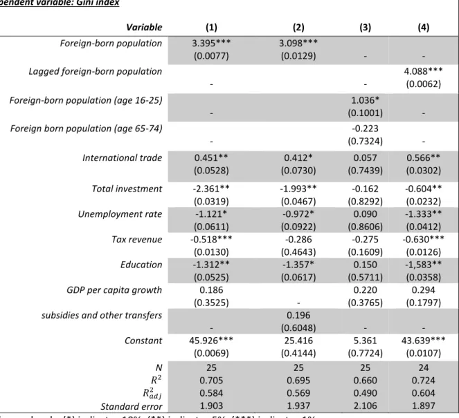
included in this table. The first model includes only foreign-born population as a measure of the total immigrants in Sweden. As one can see, this variable has a highly significant positive effect on Gini index at significance level of 1% (3.395; p-value = 0.0077). That explains the positive relationship between immigration and income inequality with the fact that, as the number of foreign-born population increases, the level of income inequality increases as well.

For the second model in table 2 we replace GDP per capita growth by subsidies and other transfers since GDP per capita growth is the only variable which is not significant in the first model. Thus, we include another explanatory variable and we see that the effect of immigration on income inequality is still highly significant.

For the third model in table 2 we divide our immigration variable into two different groups. The first group includes a group of young foreign-born population aged 16-25 and the second group includes old immigrants aged 65-74 with same explanatory

variables which were included in model 1. We see that young immigrants have a positive significant effect on the Gini index (1.036, p-value = 0.1001) at 10% significance level, i.e. immigrants of age 16 to 25 have a positive relationship with Gini index. Whereas old immigrants of ages between 65 and 74 have no significant effect on Gini index (-0.223; p-value=0.7324). This suggests that the Gini index is not affected by old foreign-born population.

Furthermore, we include the lagged-term of our main immigration variable in model 4. This is recommended by Studenmund (2017) when studying the non-instantaneous relationship between the dependent variable and the independent variables where the

(32)

28 independent variable foreign-born population is expected to affect the dependent variable

Gini index over time resulting in a change in the dependent variable. We see that including

the lagged-term of foreign-born population in the Gini index equation dramatically rises the predicated effect of immigration on income inequality. Lagged-term of foreign-born

population has also a positive and highly significant effect on income inequality (4.088; p-value=0.0062).

Table 2. Static estimation using OLS, Sweden, 1993-2017

Independent variable: Gini index

Variable (1) (2) (3) (4)

Foreign-born population 3.395*** (0.0077)

3.098***

(0.0129) - -

Lagged foreign-born population

- -

4.088*** (0.0062)

Foreign-born population (age 16-25) -

1.036* (0.1001) -

Foreign born population (age 65-74) - -0.223 (0.7324) - International trade 0.451** (0.0528) 0.412* (0.0730) 0.057 (0.7439) 0.566** (0.0302) Total investment -2.361** (0.0319) -1.993** (0.0467) -0.162 (0.8292) -0.604** (0.0232) Unemployment rate -1.121* (0.0611) -0.972* (0.0922) 0.090 (0.8606) -1.333** (0.0412) Tax revenue -0.518*** (0.0130) -0.286 (0.4643) -0.275 (0.1609) -0.630*** (0.0126) Education -1.312** (0.0525) -1.357* (0.0617) 0.150 (0.5711) -1,583** (0.0358) GDP per capita growth 0.186

(0.3525) -

0.220 (0.3765)

0.294 (0.1797) subsidies and other transfers

- 0.196 (0.6048) - - Constant 45.926*** (0.0069) 25.416 (0.4144) 5.361 (0.7724) 43.639*** (0.0107) N 𝑅2 𝑅𝑎𝑑𝑗2 Standard error 25 0.705 0.584 1.903 25 0.695 0.569 1.937 25 0.660 0.490 2.106 24 0.724 0.604 1.897 Significance levels: (*) indicates 10%, (**) indicates 5%, (***) indicates 1%

5.1.2 US

To explore the effect of immigration on income inequality in the United States, we follow same procedures as we did for Sweden, except that we do not include the lagged term of foreign-born population here. We also include four different models for US where the first

(33)

29 three models are the same from Sweden-model to make it possible to compare our results in these two countries.

We estimate the same regression model for US holding the variables the same from Sweden-model:

𝐆𝐈𝐍𝐈 = 𝜷_𝟎+ 𝜷_𝟏(𝐅𝐁) + (𝑻𝑹𝑨𝑫𝑬)𝜷_𝟐+ (𝑻𝑰𝑵𝑽𝑺𝑻)𝜷_𝟑+ (𝑼𝑹)𝜷_𝟒+ (𝑻𝑨𝑿𝑹)𝜷_𝟓

+ (𝑪𝑮𝑹𝑨𝑫)𝜷_𝟔+ (𝑮𝑫𝑷)𝜷_𝟕+ 𝜺_𝒕

Model 1 in table 3 shows that there is also a positive and significant relationship between foreign-born population and income inequality in US (0.888; p-value = 0.0895) at 10% significance level. This result shows also that immigration and income inequality are

positively correlated. However this relationship between immigration and income inequality was significant at a lower level of significance in the Sweden-model compared to the US-model. This explains that immigration affects income inequality in Sweden more than US.

Model 2 in table 3 shows the results from replacing the GDP per capita growth by subsidies and other transfers, it can be noticed that the relationship between immigration and income inequality is positive and significant at a lower significance level than the first model. However including the variable “subsidies and other transfers” make some of the other independent variables significant where none of these variables was significant in the first model when GDP per capita growth was included.

Furthermore, one can see that from model 3, when two different age groups of immigrants were included in the same model, Gini index is negatively affected by young immigrants, who are of the ages of 21 and under at significance level of 10% (-1.058; p-value = 0.0902), i.e. as the number of foreign-born population under age 21 increases, the Gini index decreases. The older population with ages 65 and over have no impact on income inequality in the United States as well (-1.508; p-value= 0.1937).

For the fourth model in table 3, we include our main immigration variable

foreign-born population with a new variable being, black population.

Since race is not that important in Sweden but is in the US, we only include this variable for US-model expecting that this variable has a positive effect on income inequality, suggesting that an increase in the black population will lead to an increase in Gini index since the black

(34)

30 population is statistically shown to earn lower income than white people, resulting in more people at the lower ends of income distribution.

Model 4 in table 3, which includes the black population variable, is shown not to be significant with high p-value (-3.446; p-value =0.3729). These results explain that black population has no significant impact on income inequality, opposing our expectations. On the other hand, including this variable in Gini index equation increases the predicated impact of immigration on income inequality compared to the first and the second model in table 3. The coefficient is 1.479 (p-value=0.0163) compared to (0.888) in model 1 and (1.361) in model 2.

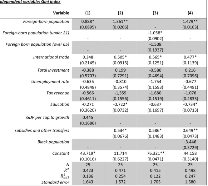
Table 3. Static estimation using OLS, US, 1993-2017

Independent variable: Gini index

Variable (1) (2) (3) (4) Foreign-born population 0.888* (0.0895) 1.361** (0.0206) - 1.479** (0.0163) Foreign-born population (under 21)

- -

-1.058*

(0.0902) -

Foreign born population (over 65)

- - -1.508 (0.1937) - International trade 0.348 (0.2145) 0.505* (0.0915) 0.565* (0.1251) 0.477* (0.1139) Total investment -0.388 (0.5707) 0.199 (0.7291) -0.580 (0.4694) 0.216 (0.7096) Unemployment rate -0.635 (0.4848) -0.810 (0.3574) -1.754 (0.1593) -0.677 (0.4491) Tax revenue -0.566 (0.4611) -1,359 (0.1556) -1.680 (0.1519) -1.076 (0.2833) Education -0.271 (0.3620) -0.722* (0.0732) -0.637 (0.1697) -0.734* (0.0713) GDP per capita growth 0.445

(0.1686) - - -

subsidies and other transfers 0.534* (0.0676) 0.586* (0.1483) 0.649** (0.0473) Black population - - - -3.446 (0.3729) Constant 43.719* (0.1016) 11.714 (0.6227) 76.321** (0.0471) 44.158 (0.3140) N 𝑅2 𝑅𝑎𝑑𝑗2 Standard error 25 0.423 0.186 1.643 25 0.471 0.254 1.572 25 0.415 0.122 1.705 25 0.498 0.247 1.580 Significance levels: (*) indicates 10%, (**) indicates 5%, (***) indicates 1%

(35)

31 5.2 Testing for Stationarity, Autocorrelation and Spurious Regression

5.2.1 Stationarity

Testing for stationarity is the fundamental criteria to examine the long-run relationship between two variables, which in this case is between immigration and income inequality. Therefore, before we begin estimating the long- and the short- run relationship between immigration and income inequality using ECM, it is crucial to check the stationarity of the variables. We check the stationarity of the Gini index as well as the stationarity of the main immigration independent variable foreign-born population. We use Dickey-Fuller test for this purpose, and we estimate the following equations using OLS:

For testing the stationarity of the dependent variable Gini Index Δ𝐺𝑖𝑛𝑖𝑡= 𝛽0+ 𝛽1𝐺𝑖𝑛𝑖𝑡−1+ 𝜀𝑡

For testing the stationarity of the independent variable Foreign-born population Δ𝐹𝐵_𝑡= 𝛽₀+ 𝛽₁𝐹𝐵_𝑡−1+ 𝜀_𝑡

Results from estimating these two equations are presented below in table 4.

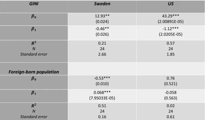
Table 4. Testing the stationarity of variables, Dickey-Fuller Test

GINI Sweden US 𝜷𝟎 12.93** (0.024) 43.29*** (2.00891E-05) 𝜷𝟏 -0.46** (0.026) -1.12*** (2.0205E-05) 𝑹𝟐 N Standard error 0.21 24 2.66 0.57 24 1.85 Foreign-born population 𝜷𝟎 -0.53*** (0.010) 0.76 (0.521) 𝜷𝟏 0.068*** (7.95033E-05) -0.058 (0.563) 𝑹𝟐 N Standard error 0.51 24 0.16 0.02 24 0.61 Significance levels: (**) indicates 5%, (***) indicates 1%

(36)

32

As one can see, the estimated beta (𝛽̂) for the Gini index is significantly less ₁

than zero for both Sweden and US which leads to that the null hypothesis of a unit root can be rejected and thus that implies that Gini index is stationary.

Moreover, the results for the foreign-born population variable show that (𝛽̂) 1

is not significantly less than zero for both countries, where 𝛽̂ is negative but not significant 1

for US- model, and it is positive and significant in Sweden-model which implies that the foreign-born population is nonstationary in both Sweden and United states since the null hypothesis of a unit root cannot be rejected in that case.

5.2.2 Autocorrelation2

The usage of time series data occasionally brings upon the risk of an econometric complication called autocorrelation, i.e. correlated observations of the error term. The stochastic error term is often affected by events that took place in a previous time period when using time series multiple regression (Studenmund, 2017). To test for this, we use Durbin-Watson test for our static model in both Sweden and US to test if there is a positive autocorrelation. This test cannot be used for our dynamic model since the dynamic model is estimated using error correction model which includes a lagged dependent variable as an independent variable.

Given that the null hypothesis of no positive autocorrelation and a one-sided alternative hypothesis of positive autocorrelation, the decisions rule of the Durbin-Watson test is as follows:

𝑑 < 𝑑𝐿 𝑅𝑒𝑗𝑒𝑐𝑡 𝑛𝑢𝑙𝑙 ℎ𝑦𝑝𝑜𝑡ℎ𝑒𝑠𝑖𝑠 𝑑 > 𝑑𝑈 𝐷𝑜 𝑛𝑜𝑡 𝑟𝑒𝑗𝑒𝑐𝑡 𝑛𝑢𝑙𝑙 ℎ𝑦𝑝𝑜𝑡ℎ𝑒𝑠𝑖𝑠 𝑑𝐿≤ 𝑑 ≤ 𝑑𝑈 𝐼𝑛𝑐𝑜𝑛𝑐𝑙𝑢𝑠𝑖𝑣𝑒

Where d is calculated by using the equation for the Durbin-Watson statistics for T observations 𝑑 = ∑ (𝜀𝑡 − 𝜀𝑡−1) 2 𝑇 2 ∑ 𝜀𝑇 _𝑡2 1

And 𝑑𝑈, 𝑑𝐿 are the critical values for the Watson statistics. We conduct the

Durbin-Watson test for autocorrelation for each of the countries we have, beginning with table 2,

2_{We also tested for heteroskedasticity using Breusch-Pagan Test since heteroskedasticity is also supposed to be}

The Impact of Immigration on Income Inequality : Evidence from Sweden and the United States