Production optimization for district heating : Short-term planning of district heating grid in Gävle, Sweden

DISTRICT HEATING

Short-term planning of district heating grid in Gävle, Sweden

KARL BROGREN

NICOLAS LINDGREN

The School of Business, Society and Engineering Course: Degree project in Sustainable Energy

ii

ABSTRACT

Energy systems with a high portion of renewable energy from wind and solar power can suffer from fluctuations in production due to weak winds or cloudy weather, which may affect the electricity price. When producing heat and power in a combined heat and power plant, an additional heat storage tank can be used to store the heat surplus which is obtained when the power production is high, and the heat demand is low. To optimize heat and power production economically, short-term planning can be applied. Short-term planning covers the production in the near future of 1-3 days. The optimization in this degree project is based on the district heating production, which means that the heating demand always needs to be fulfilled. The district heating production is based on the weather. Therefore a suitable period for simulation is three days due to the accuracy of the weather forecasts are reasonable. The optimization is performed on the district heat system in Gävle, Sweden. The system comprises several different production units, such as combined heat and power plants, backup plants, and industrial waste heat recovery. Two different models are made, one using linear programming and one using mixed integer non-linear programming. The model stated as a linear programming problem is not as accurate as of the one stated as a mixed integer non-linear programming problem which uses binary variables. Historical input data from Bomhus Energi AB, a company owned together by the local heat and power supplier Gävle Energi AB and the pulp and paper manufacturer BillerudKorsnäs AB, was given to simulate different scenarios. The different scenarios have various average temperatures and in some scenarios are there some issues with the pulp and paper industry affecting the waste heat recovery. In all scenarios is the heat storage tank charged when the demand is low and then discharged when the demand increases to avoid starting some of the more expensive backup plants if possible. The simulation time varies a lot between the two approaches, from a couple of seconds to several hours. Particularly when observing scenarios with a rather high demand since the backup generators use binary variables which take a lot of time to solve.

Keywords: Short-term planning, Optimization, District heating, Linear programming, Mixed integer non-linear programming, Branch and bound, Heat storage, MATLAB, TOMLAB

PREFACE

We want to thank our supervisor Jan Skvaril at Mälardalens Högskola, for providing us with guidance throughout the work. We would also like to express our happiness for making this project possible as our degree project, thank you EnviLoop AB and Bomhus Energi AB. Inspiration for the project has been Erik Dotzauer and the work he has done in the area of study. Therefore we would like to thank him.

Västerås May 2019

Karl Brogren Nicolas Lindgren

iv

SUMMARY

Renewable energy systems such as wind and solar power may affect fluctuations in the power grid caused by weak winds and cloudy weather. The fluctuations in the power grid can affect the electricity price. Producers at combined heat and power plants want to produce electricity when the price is high to increase the revenues. When producing electricity, a significant amount of heat is produced as a by-product. The heat is often inserted to a district heating grid. If the amount of produced heat exceeds the heating demand, the heat surplus must be stored to remain a high efficiency.

The purpose of this degree project is to develop a process model that can optimize how the production units should operate and how the heat storage tank should be charged and discharged to provide the best economic outcome. The model is based on a prognosticated heat demand, which must be fulfilled.

To get a better understanding of the problem as well as finding suitable approaches to solve the problem is a comprehensive literature study made. Most of the information is gathered from a similar research project, scientific papers, and books related to the field. The primary databases used to find scientific papers and research projects are Google Scholar, Research Gate, and Science Direct. A study visit to the different facilities in Gävle is made to gain a better understanding of the production units and the distribution system. To get relevant input data about the various production units, a meeting with the process engineers at BillerudKorsnäs AB, Bomhus Energi AB, and Gävle Energi AB is held. The input data have a central role in the development of the model.

The model is created in MATLAB. It runs the main script, which calls on several functions related to the production units and the optimization. Since the problem is rather complex, several different solvers are used in the optimization function. Which solver to use is highly dependent on the problem formulation. If the problem is stated as a linear programming (LP) problem, a more straightforward solver can be used, which reduces the accuracy of the model. If the problem, on the other hand, is stated as a mixed integer non-linear programming (MINLP) problem, the model can be more accurate but demands a more advanced solver. To validate the model, a sensitivity analysis is made. The sensitivity analysis is performed by changing the input data and observe the result to control if it behaves in a correct and anticipated way. The different input data are related to different scenarios. The scenarios vary in heat demand and production status of the pulp and paper industry.

The optimized production process uses cheaper production units as a base load, and when the heat demand is low, the heat storage tank charges. When the heat demand is increased, the tank discharges to avoid starting the more expensive backup plants if possible. When comparing the simulation with and without heat storage, the simulation, including heat storage has a lower cost.

When the model is compared to the previous model used at Bomhus Energi AB, the result shows that for a specific scenario, the savings are around 400 000 SEK, both for the LP-model and the MINLP-model.

It is primarily the use of the backup units that differs between the linear and the non-linear approach. Which make the result of the linear and the non-linear model the same when the heating demand is low. Since the non-linear problem can be solved as a linear problem. The variation in run time for the simulation is rather significant between the two approaches, specifically when the demand is high. It can range from a couple of seconds for the linear solver to above 1 000 seconds for the non-linear solver.

The work concludes that the linear model is a more practical tool for the customer while being a bit less realistic when it comes to the result. The new model is an improvement from the old and helps to avoid unnecessary costs.

TABLE OF CONTENT

1.6 Contribution to current research ...11

2 METHOD ... 12

2.1 Gathering of data ...12

2.2 Modeling and simulation ...12

2.3 Validation of result ...13

3 LITERATURE STUDY ... 14

3.1 Thermal storage ...14

3.2 Optimization of a CHP-plant with a heat storage unit ...16

3.3 Modeling of non-linear efficiencies ...18

3.4 Non-convex & non-continuous problems ...19

3.5 Branch and bound optimization ...20

4 MODELING ... 23

4.1 Existing model ...23

4.2 Current model ...23

4.3.1 Linprog ...24

4.3.2 TOMLAB ...24

4.3.2.1. MinlpBB ... 24

4.4.1 Linear programming ...25

4.4.2 Mixed-integer non-linear programming ...28

4.5 Scenarios ...30 5 RESULT ... 31 5.1 Linear vs. Nonlinear ...33 5.2 Heating Demand ...35 5.3 Electricity Price...36 5.4 Storage vs. No storage ...37

5.5 Bomhus Energi model vs. Minlp model ...39

6 DISCUSSION... 41

7 CONCLUSION ... 44

8 FURTHER WORK ... 45

REFERENCE LIST ... 46

APPENDIX 1. LINEAR PROGRAMMING ... 50

APPENDIX 2. MIXED INTEGER NONLINEAR PROGRAMMING ... 55

APPENDIX 3. NONLINEAR CONSTRAINTS (MINLP) ... 63

APPENDIX 4. OBJECTIVE FUNCTION (MINLP) ... 64

INDEX OF FIGURES

Figure 1 Black liquor evaporator with three effect stages ... 9

Figure 2 Simplified block scheme of steam production for the district heating grid and industries ... 10

Figure 3 Flowchart of the simulation process. ... 13

Figure 4 Load shedding of a district heating system (Frederiksen & Werner, 2014) ... 15

Figure 5 Pressureless heat storage tank connected to a district heating grid. (Frederiksen & Werner, 2014) ...16

Figure 6 Example of convex sub-models, 9 points (Makkonen & Lahdelma, 2005) ... 20

Figure 7 Enumeration tree related to the example. (Vanderbei, 2014) ...21

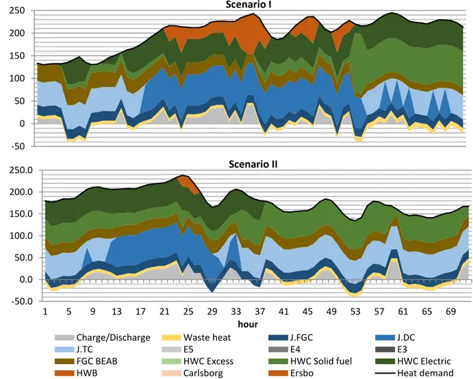
Figure 8 Minlp result for scenario I & II ... 31

Figure 9 Minlp/lp result for scenario III, IV & V ... 32

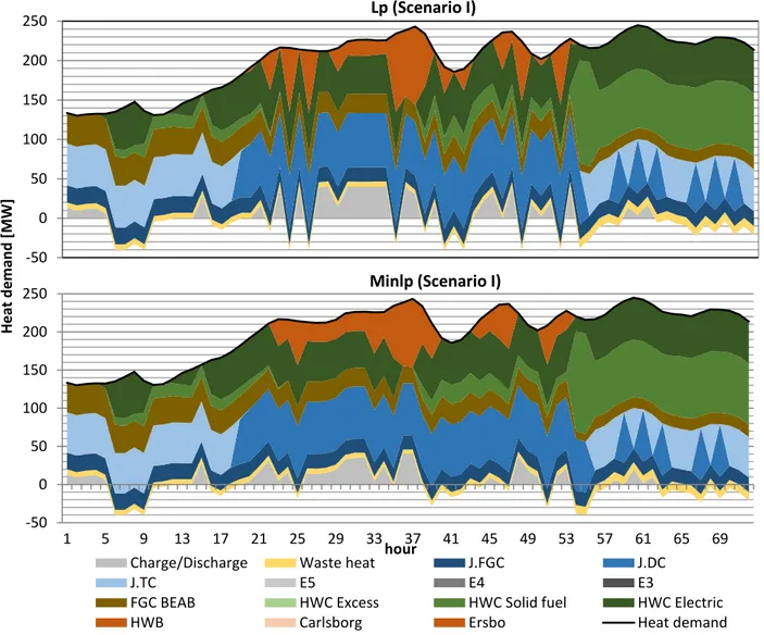
Figure 10 Comparison of scenario I minlp and lp result. ... 33

Figure 11 Comparison of scenario II minlp and lp result ... 34

Figure 12 In/Decrease heat demand for scenario I. ... 35

Figure 13 In/Decrease electricity price for scenario I. ... 36

Figure 14 Comparison of production costs for different production units at different electricity prices. ... 37

Figure 15 Scenario III, storage vs. no storage ... 38

Figure 16 Previous vs. Minlp model ... 39

Figure 17 Total production cost comparison between the Bomhus model, the Minlp model, and the Lp model... 40

Figure 18 Previous vs. Minlp model ... 65

INDEX OF TABLES

Table 2 Cost comparison scenario I different electricity prices ... 37

Table 3 Scenario III, storage vs. no storage ... 38

NOMENCLATURE

Denotation Description Unit

P Power Watt [W] Q Heat Watt [W] t Temperature Celsius [°C] η Efficiency Percent [%] i Timestep Hour [h]

ABBREVIATIONS

BEAB Bomhus Energi AB

CHP Combined heat and power

Evap Evaporator

FGC Flue gas condenser

GEAB Gävle Energi AB

HWB Hot water boiler

HWC Hot water condenser

IP Integer programming

J Johannes combined heat and power plant

LP Linear programming

MILP Mixed integer linear programming MINLP Mixed integer non-linear programming MIP Mixed integer programming

DEFINITIONS

Definition Description

A Inequality constraints matrix Aeq Equality constraints matrix B Inequality constraints vector Beq Equality constraints vector

Black liquor Black liquor is a waste product from digesting

pulpwood, from the process of producing paper pulp. fT _{Transposed objective}

Kraftliner Paperboard made from virgin pulp

lb Lower bound vector

Load

shedding Store heat when the demand is low, utilize stored heat through discharging when the demand is high. Scenario I Big operation problems with the industry, going into a

period with cold weather.

Scenario II Big operation problems with the industry, going into a period with warmer weather.

Scenario III Regular operation, significant variations in

temperature during night and day. Temperatures are below 0°.

Scenario IV Regular operation, warm weather.

Scenario V Regular operation, significant variation in temperature during night and day. Temperatures are above 0°.

SOS Special ordered set, Thermal

stratification Keep the stored water layered by temperature, warm water in the top and cold water in the bottom.

ub Upper bound vector

1

INTRODUCTION

The rising awareness about human-caused emissions and its effects on the environment and human health has led to investment towards a more environmentally friendly energy system (Karaoğlan & Durukan, 2016).

Energy systems with a high portion of renewable energy from wind and solar power can suffer from fluctuations due to cloudy weather or weak winds. The variations also affect the electricity price. (Pappala, Erlich, Rohrig, & Dobschinski, 2009; Garcia-Gonzales, Moraga.R, Santos.M, & Gonzales.M, 2008)

To eliminate the fluctuations in the grid, combined heat, and power (CHP) plants, together with a heat storage unit, is a practical solution. The heat and power production of a CHP-plant can easily be regulated to match the fluctuations in the grid. (Mueller, Tuth, Fischer, Wille-Haussmann, & Wittwer, 2013)

A high electricity production provides a high production of heat that could exceed the heat demand. With a heat storage unit, the heat surplus can be stored, and therefore, also maintain a high total efficiency, which characterizes a CHP-plant (Abdollahi, Wang, Rinne, & Lahdelma, 2014). CHP-plants can use biofuels to be more environmentally friendly than it would be using fossil-based fuels. A deregulated electricity market, which is existing in Sweden, makes the electricity production competitive and leads to a more volatile price (Swedish Competition Authority, 1996). Due to this, dynamical decision tools are essential to cover the heat demand while maximizing the profits.

Today most of the long-term contracts have been replaced by term contracts. The short-term contracts put certain requirements on the production, which must be optimized with high precision to be able to meet the varying electricity price while covering the heating demand (Energimarknadsinspektionen, 2015). To get the future heating demands, prognostication of the weather must be made since the demand for heat is entirely dependent on the weather. However, the weather forecasts for long periods are rarely as accurate as they need to be (Monache.D, 2010). Because of this, the prognostication must be valid and needs to be updated continuously to get the best possible accuracy.

In this degree project, a premade prognostication model is used to help improve the current production optimization tool where the heat storage unit is not considered. The district heating system to optimized is located in Gävle, Sweden, where Gävle Energi AB owns the district heating grid.

to Sweden’s national grid. During a normal year, the power produced from these hydropower plants is 56 GWh. (Gävle Energi, 2019) In addition to these hydropower plants, there are two combined heat and power plants (Bomhus & Johannes), two heat only plants (Carlsborg & Ersbo) and a pulp and paper industry (BillerudKorsnäs) where heat is recovered from various processes to the district heating grid. These facilities supply Gävle with heat during the entire year. The base load for heat production is the waste heat from the industry, BillerudKorsnäs, and when this is not enough to cover the demand the CHP-plants can help to meet the demand (Gävle Energi, 2019). Johannes CHP-plant has a production capacity of 23 MW power and 77 MW heat with flue gas condensing included. (Bomhus Energi, 2019) The fuel used in Johannes is biofuel, consisting mainly of bark and recycled wood (Gävle Energi, 2019). A heat storage unit is also present at Johannes, which creates the possibility to store heat for later, increasing the flexibility of the CHP-plant. The storage unit can divert a part of the incoming district heating flow, heat it and then send it to the outgoing water in the district heating grid, where it is mixed with the water heated in the condenser at Johannes. During the coldest days or when the primary facilities are not available two back-up heat plants, Ersbo and Carlsborg can be used to meet the heating demand. Both back-up plants use bio-oil as their fuel. Ersbo has a capacity of 80 MW and Carlsborg 60 MW. (Bomhus Energi, 2019)

1.2

Bomhus Energi AB

Bomhus Energi AB (BEAB) was founded in 2010 as a result of a cooperation between the municipality owned Gävle Energi AB and the paper industry BillerudKorsnäs AB. Both parties own 50% each of BEAB. The CHP-plant is located in the same area as the paper industry. Gävle Energi AB and BillerudKorsnäs AB decided not to build one boiler each but instead build a conventional boiler which became BEAB with the purpose to secure the steam production needed for the paper industry, the sawmill located nearby, and supply heat to the district heating grid when possible and needed. The industries require steam at two pressure levels, 4 and 12 bar. (Bomhus Energi, 2014) BillerudKorsnäs produce single-use portion liquid packaging’s, and white top kraftliner. Kraftliner is a paper product that is used in the outermost layer of corrugated fiberboard (Skogen, n.a.). The total production is 740 000 tons every year. (BillerudKorsnäs, 2019) The business is competitive and requires a high-quality product, making it important to deliver the steam it needs (Confederation of European paper industries, 2006; Karikallio, Mäki-Fränti, & Suhonen, 2011). Electricity is also produced from Bomhus but is seen as a co-product to increase the total efficiency since the produced heat is the primary product. The CHP-side consists of a biofueled boiler and a turbine from Siemens. The turbine has a nominal power of 92 MW, and maximum heat production from the condenser is 150 MW with flue gas condensing not included. The primary fuel used for the boiler is bark. (Bomhus Energi, 2019)

Besides the bio-fueled boiler, there are two recovery boilers and two electrical boilers that can produce steam. The recovery boilers are a part of the paper industry and help the chemical cycle by recovering chemicals from the black liquor which is a waste from digesting pulpwood, by combusting the organic substances that comes from the wood chips in the treatment process

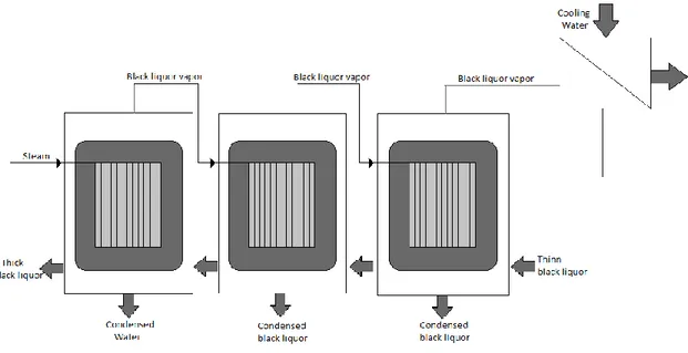
(Bomhus Energi, 2019). Another process where heat is recovered is from the black liquor evaporators. After the black liquor has been separated from the pulp fiber from the digesters and pulp wash, the black liquor contains too much water to be used as fuel in the recovery boilers (Bomhus Energi, 2019). Bergsten (2015) describes the process as the following, to decrease the moisture level of the black liquor, a series of evaporators is used. These evaporators are called effect stages. One effect stage is made up of one or more evaporators operating with the same pressure level. The most common approach is to use subatmospheric pressure, this to make the evaporation process easier, the further it gets. In the first effect stage steam is used to evaporate the moisture in the black liquor, then the steam is directed away, and its heat is recovered to the district heating grid. The next effect steps use the evaporated black liquor as the hot fluid. Therefore, a lower pressure is required in the other effect stages. A higher number of stages require a lower amount of steam compared to a lower number of effect stages. The sub-atmospheric pressure is created by a condenser that cools the liquor vapor in the last effect step. Figure 1 illustrates an example of three effect stages. From the condenser that chills the liquor vapor medium temperate water is produced. For the highly contaminated liquor condensate, a large portion of combustible organic material that can be separated from the water using a distillation process, this is done in a stripping column.

Figure 1 Black liquor evaporator with three effect stages

The electric boilers have a total production capacity of 80 MW, and its primary purpose is to be used as a backup when needed but, it can also be one of the more cost-effective ways to produce steam when the electricity is cheap. The paper industry also has an oil-fired backup boiler with a capacity of 110 MW. In the system, there is a steam accumulator that can store

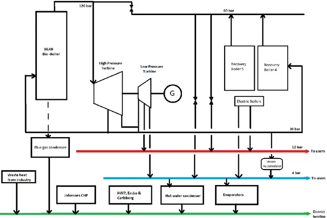
Figure 2 Simplified block scheme of steam production for the district heating grid and industries

1.3

Purpose

The purpose of the project is to develop a process model that can, from a prognosticated heat demand, provide guidance and decision support of how the facilities should be operated to provide the best possible economic outcome, in terms of minimizing the production cost which involves revenues from sold electricity. Which also includes the heat storage unit as well, when to charge it and when to discharge it.

1.4

Research questions

 How should the heat storage unit in Johannes be operated, in terms of charging and discharging, to get the best economic outcome while meeting the heat demand during the simulation period of 3 days?

 What is the optimal mix of boiler loads to meet the heat demand and gives the lowest production cost and highest profit?

1.5

Delimitations

The power production from the CHP-plants is not researched since the heat production is the main product, and the electricity is seen as a by-product. Forecasting of the heat demand and electricity price is already developed by Gävle Energi and is not studied. The simulated period is delimited to 3 days since the heat demand forecast is based on the weather forecast. In order to meet the heating demand, a specific feed temperature should be required. However, in this study, only the needed energy is observed. Some delimitations in costs for additional software are taken into consideration. Due to the end model being developed for a customer, the choice of software must be accepted by the end user and be within a reasonable price.

1.6

Contribution to current research

The contribution of this degree project is to provide a simulation model related to the district heating grid in Gävle. The modeling methodologies that are described in the literature study are not immediately suitable for the problem related to this degree project, in terms of planning period and number of production units. Therefore, a new approach is undertaken to solve the problem for this specific district heating grid.

2

METHOD

In this section, is the methodology about the gathering of data and the simulation model explained.

2.1

Gathering of data

A comprehensive literature study was made in order to get a better understanding of the problem as well as finding different methods to solve the problem. Most of the information about suitable approaches to solve the problem is gathered from similar research projects and scientific papers found in the databases Google Scholar, Research Gate, and Science Direct. The general information about energy storage and basic mathematics is gathered from books. In order to find relevant scientific papers, some specific search parameters were used, knowing it is a widely used term in the problem area. Unit commitment, economic dispatch, short-term planning of district heating, and cogeneration are some phrases that were used commonly to find information. After searching for information, some names were seen a lot in different papers handling the same issues, giving the impression they have had a significant influence on the industry. More papers were found by using the frequently appearing names.

A study visit to the different facilities was made to gain a better understanding of the production units and the distribution system. Relevant input data about the various production units were gathered during a meeting with the process engineers at BillerudKorsnäs AB, Gävle Energi AB, and Bomhus Energi AB. The collected data have a central role in the development of the model.

2.2

Modeling and simulation

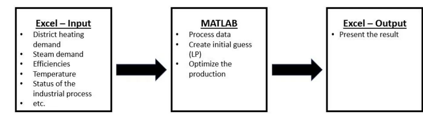
The model was created with MATLAB. The base model runs the main script which reads the input data including the prediction of the district heating demand and electricity market price from an excel file, then it calls on functions for all production units and one optimization function, the process is explained in Figure 3 below. Since the problem is rather complex, several different solvers are used in the optimization function. Which solver to use in the optimization function is highly dependent on the problem formulation. If the problem is simplified to a linear programming (LP) problem, a more straightforward solver can be used, which reduces the accuracy of the model. If the problem, on the other hand, is stated as a mixed integer non-linear programming (MINLP) problem, the model can be more accurate, and a more advanced solver is needed.

Figure 3 Flowchart of the simulation process.

2.3

Validation of result

Since there is no data to compare the result with, other measures must be used to ensure that the result is the global optimum, and not a local. If the objective function is convex, only one optimum exists. Validation of the model was done by using the same approach as previous projects with similar scope, and by performing a sensitivity analysis. The sensitivity analysis was performed by changing input data and observe the result to control if it behaved the correct and anticipated way.

3

LITERATURE STUDY

In the following chapter will the technical information relevant to this project be presented. A reference to Erik Dotzauers article from 1997 is used as a base for this project. This is motivated by that the mindset on how to simulate/operate a plant is not changed since. Therefore, the same constraints can be used to get a valid simulation model. Also, it is confirmed by recent articles using the same methodology. Chenghong, Da, Junbo, Xitian, and Qian (2015) confirms that a CHP plant is either operated after the electricity or heat load. In this work is it the heat load that decides the production, Dotzauer (1997) uses the same strategy. All images with references have been approved by their respective authors to be used in this work.

3.1

Thermal storage

According to Frederiksen and Werner (2014), large scale thermal storage is often divided into two methods, short-term storage, and seasonal storage. The seasonal storage method is under progress and is often related to thermal solar power. Short-term storage is, however, a well-established method whose purpose is to:

 Push the load from a period when the demand is high to a period where the demand is lower.

 Reduce rapid load changes that can harm the production unit.

 Avoid energy losses which are related to frequent start and stops of the production unit.

 Increase the production of electricity when, for example, the demand for cooling is higher than the demand for heat.

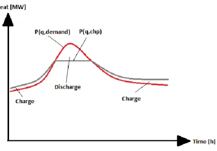
In Figure 4, the load shedding for a district heating system presented. The storage tank discharges when the heating demand is higher than the available heat production.

Figure 4 Load shedding of a district heating system (Frederiksen & Werner, 2014)

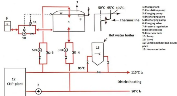
In a district heating system is the most common method for thermal storage, the short-term storage method which bases on thermal stratification. Thermal stratification occurs when the temperature of the water increases which decreases the density of the water, which in turn makes the mass of hot water lay on top of the mass of cold water (Frederiksen & Werner, 2014). In order to avoid stratification degradation and to improve the storage cycle performance must the injection, recovery, and holding of heat be managed carefully (Dincer & Rosen, 2012). Figure 5 which according to Frederiksen and Werner (2014) explains a pressureless hot water storage tank (1) which is connected to a district heating grid. The storage tank is connected in series with a combined heat and power plant (12) and a backup boiler (13). In the figure, two parallel circuits are presented, in order to charge the tank, open the charging valve (6) and start up the charging pump (3). To discharge the tank, open the discharge valve (4) and start the discharging pump (4). The water level in the tank remains stable by the circuit including a pump (10) and a valve (11), when the water level is to low the pump startup and pump water from the reservoir tank (9), and when the water level is too high the valve is opened in order to transport water to the reservoir.

Figure 5 Pressureless heat storage tank connected to a district heating grid. (Frederiksen & Werner, 2014)

3.2

Optimization of a CHP-plant with a heat storage unit

When planning district heating production, it is critical that there is a time perspective considered, especially if there is a heat storage unit involved. According to Dotzauer (1997), the time perspective can be divided into three levels, long-, medium-, and short-term production planning. The long-term planning involves decisions about future investments, including production capacities and expanding the district heating grid in a coming period of 5-25 years. Medium-term planning handles fuel and electricity contracts in the next coming 1-5 years. Short-term planning is about finding the optimal operation conditions for the facilities in a period from 1 – 7 days. (Dotzauer, 1997; Salgado & Pedrero, 2008) Commonly it is divided into subproblem for each production unit, and to increase the accuracy of the planning the period to be solved should be for the upcoming 24 hours (Dotzauer, 1997). Frederiksen and Werner (2014) describe the benefits of short-term planning as is it giving lower marginals for fuel consumption and a higher precision electricity production of a CHP-plant. Today the market for electricity requires that all producers of power must report their planned production for the next coming day. This helps to balance the supply and demand. (Frederiksen & Werner, 2014) It is crucial that the unit is being operated in an optimal condition in order to reduce cost, especially plants where the production cost is high (Dotzauer, 1997; Frederiksen & Werner, 2014), for example, oil-fired boilers. For a plant with a high production cost, a lot of money can be saved daily (Dotzauer, 1997). The optimal operating conditions also help to reduce unwanted emissions, which also help reduce costs. With an increasing number of production units and heat storage units, the complexity and difficulty to

find the optimal operating conditions also increase rapidly. From Erik Dotzauers (1997) analysis for optimal operation, the below-described aspects are what complicates the problem and must be taken into consideration.

 With several production units, it can be hard to decide which ones that should be used as a baseload, it limits the minimum operation- and downtimes of the plants. The minimum operation time is the time that the plants must be operated if started, and minimum downtime is the time the plant must be off if the operation is shut down. This must be considered because there is a start-up cost for the plants that affect the optimization. Dotzauer calls this problem of which unit should be operated and which should be off “the unit commitment problem”. The term is widely used in the sector and is extensively researched in its community (Pandžić & Luburić, 2019; Fossati, 2012).

 If any of the units that are optimized are combined heat and power plants, further problems appear, such as deciding the electricity production. In Sweden, the electricity is sold on an open market, Nord Pool (Energimarknadsbyrån, 2019), and the general goal is to maximize electricity production when the price for electricity is high. A CHP-plant has its highest overall efficiency at a proportional production of heat and power. This means that when electricity production is high, then heat production also is at high levels. If the produced heat exceeds the demand, problems may arise.

 With a heat storage unit, the production flexibility increases, due to that the excess heat from high electricity production can be stored for later when the electricity price is low, and the operation wants to avoid producing a small amount of electricity and high amount of heat to keep the total plant efficiency high. This tactic helps to even out peaks of the heat demand. However, when performing the optimization, this instantly increases the difficulty because a highly time-dependent aspect is introduced.

 The outline of the district heating grid has a significant influence on how the plant can produce heat since a high incoming temperature decreases the efficiency of a plant drastically, therefore it is essential that the heating grid is not connected in series but rather to use substations to deliver and distribute the heat.

To solve this complex problem, a combination of mathematical models and fitting algorithms are required. Bellqvist and Olofsson (2012) used the software GAMS and reMIND to solve the problem of similar nature at Luleå Energi AB and Lulekraft. The model made in GAMS used mixed integer non-linear programming (MINLP) and the model in reMIND mixed integer linear programming (MILP). Vennström (2014) at Umeå University also used the MILP to solve such a problem. Dotzauer (1997) has used Matlab combined with toolboxes from TOMLABs NPSOL to solve a short-term planning problem. Gopalakrishnan and Kosanovic (2015) used a genetic algorithm to solve their operational planning of a CHP with a mixed

 Linear or non-linear  Convex or non-convex

A linear problem that has both continuous and integer variables are viewed as a MILP, and if the problem is non-linear with continuous and integer variables makes it a MINLP. (Klanšek, 2014) Below a couple of methods that can be used to solved MILP and MINLP are shown (Dotzauer, 1997).

 Dynamic programming  Heuristic methods  Branch and bound  Lagrangian relaxation

3.3

Modeling of non-linear efficiencies

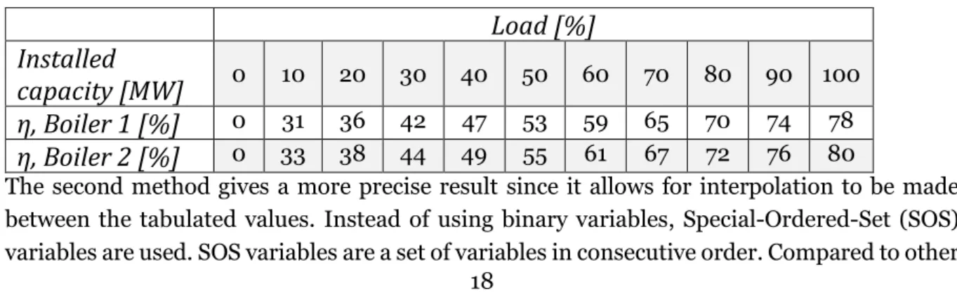
By using non-linear efficiencies, the credibility and accuracy of an optimization increases, compared to constant or linear efficiencies, this because it better reflects the real efficiencies (Tveit, Savola, & Fogelholm, 2005). The efficiencies are highly dependent on the installed capacity and the load, therefore, both these variables can be seen as the main controlling variables for the efficiencies (Milan, Stadler, Cardoso, & Mashayekh, 2015). Dotzauer (1997) shows how a secondary polynomial equation can be approximated to describe non-linear efficiencies. This requires empirical data to be available. To get empirical data, the plant can be operated in an off-design mode (Savola & Keppo, 2005). Operating the plant in off-design mode means that different parameters are changed to see how the rest of the system is affected, while still meeting a production target (Kupecki, 2015). Milan et al. (2015) describe two methods for non-linear modeling efficiencies. Both ways use linearization of the non-linear curves. The first approach uses binary variables. From the efficiency curve, a matrix is created where different loads are connected to particular efficiencies, Table 1.

The binary variables create classes, and every binary variable is related to a specific value in the matrix. When the actual load is known, the efficiency is found by finding the nearest located load in the matrix. This does not give the exact efficiency because interpolation between tabulated values does not work with the binary variables. However, it is a simple solution to avoid using constant efficiencies.

Table 1 Example of efficiencies at different loads

Load [%]

Installed

capacity [MW]

η, Boiler 1 [%]

η, Boiler 2 [%]

The second method gives a more precise result since it allows for interpolation to be made between the tabulated values. Instead of using binary variables, Special-Ordered-Set (SOS) variables are used. SOS variables are a set of variables in consecutive order. Compared to other

variables, only one (SOS1) or two (SOS2) adjacent elements in the ordered set can be set to a non-zero value. SOS variables can be used as weighting factors in linearization methods, by setting its upper and lower bounds to one and zero, respectively. Using the variables as weighting factors, a tabulated, or an interpolated value between two loads in the table can be retrieved. However, SOS-variables requires a MILP-method that supports this type of variable. Milan et al. (2015) use the CPLEX solver in the software GAMS to perform the optimization. In order to find the correct boiler (row) in Table 1, SOS1 is used, and to perform the interpolation SOS2 is used. The most accurate way of modeling the non-linear efficiency is to curve fit an equation from empirical data (Savola & Keppo, 2005).

3.4

Non-convex & non-continuous problems

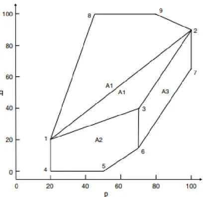
There are problems whose characteristics cannot be assumed to be convex, a problem like this is, for example, modeling of non-linear efficiencies (Makkonen & Lahdelma, 2005). If the model has linear efficiencies, it leads to the production mix of heat and power being non-convex. A non-convex model also results in there being local optimums, which can be a problem (Chun-lung, 2007). The characteristics for a modern CHP-plant is often non-continuous due to reasons such as backpressure production, the possibility to use different types of fuels and a high variety of operations modes, this in turn also makes it non-convex (Makkonen & Lahdelma, 2005). There are several ways to simplify this problem. One method is to divide the model into several convex sub-models. The sub-models are then modeled to be alternative components, and only one sub-area can be operated at a time (Rong & Lahdelma, 2007), Lien and Amato (2004) call this convex decomposition. Convex decomposition is a common way of handling non-convex problems and helps most algorithms to perform better (Lien & Amato, 2004). Makkonen and Lahdelma (2005) describe an example of a CHP-plant with a backpressure turbine with a bypass control valve, condenser, and an additional cooling unit. Altogether, this creates nine specific points, Figure 6.

Figure 6 Example of convex sub-models, 9 points (Makkonen & Lahdelma, 2005)

Figure 6 shows the heat produced as a function of power production, which Makkonen and Lahdelma (2005) explains as the following. Point 1 - 2 is the backpressure line, meaning that if the heat production should increase the bypass valve should be opened accordingly to get the wanted increase of heat, this also leads to a decreased power production due to less steam passing the turbine. Opening the bypass valve pushes the state towards points 8 and 9. However, in a reversed situation, increased power production, the current state is pushed downwards to point 3. This production mix lowers the total efficiency. If even more power is required and the cooling capacity of the condenser is not enough, the additional cooling unit is needed, the production state is pushed towards four to seven, and even further reduces the total efficiency. The total area of the graph in Figure 6 is non-convex, therefore by dividing the area into smaller parts it can be made convex, each area represents a sub model (Makkonen & Lahdelma, 2005).

3.5

Branch and bound optimization

According to Vanderbei (2014), many real-world problems can be modeled as linear programs except that some or all variables are constrained to be integers. One technique for solving problems described as integer programming (IP) problems or mixed integer programming (MIP) problems is the branch-and-bound method. The branch-and-bound method can solve a potentially large number of linear programming (LP) problems in its search for an optimal solution. The algorithm starts by ignoring the integer constraints to solve the problem and

hope that the solution vector satisfies the integer constraints. The hopes for this first solution are almost always unfulfilled, and a backup strategy is required. The backup strategy is to develop a tree of linear programming subproblems. Consider the following example.

max 𝑥₁,𝑥₂ 17𝑥1+ 12𝑥2 𝑠. 𝑡. 10𝑥1+ 7𝑥2≤ 40 𝑥1+ 𝑥2≤ 5 𝑥1, 𝑥2 ≥ 0 𝑥1, 𝑥2 𝑖𝑛𝑡𝑒𝑔𝑒𝑟𝑠

The linear programming problem obtained when the integer constraints are ignored, is called the LP-relaxation. The solution to the LP-relaxation is at (x1, x2) = (5/3, 10/3) which gives the optimal objective value 205/3 = 68,33. By rounding each component of this solution to the nearest integer gives (x1, x2) = (2, 3), which is not feasible. The closest feasible integer solution to the LP-relaxation is (x1, x2) = (1, 3) which is not the optimal solution. As mentioned, x1 for the LP-relaxation problem is 5/3. Therefore, the optimal solution to the integer problem satisfies either x1 ≤ 1 or x1 ≥ 2. Let P1 denote x1 ≤ 1 and P2 denote x1 ≥ 2. A tree of LP subproblems can now be made as in Figure 7 below, this is called the enumeration tree. The algorithm explores branches of the tree, and every branch is checked against an upper and lower bound, hence the name Branch-and-Bound.

the one for P1, the procedure must continue. The process is moving on until the last step where two integer solution is achieved, which is in P7 and P8 where P8 is highest and said to be the optimum. P7 must not be an integer but to stop the procedure, should it be lower than P8. According to Leyffer (1999), the same methodology can be used for solving mixed integer nonlinear programming (MINLP) problems. All integer constraints are relaxed, and the resulting nonlinear programming problem is solved. If the solution is an integer solution, the algorithm stops. If not, the algorithm continues by creating an enumeration tree with branches that are checked against lower and upper bounds. The branch and bound algorithm is a global optimization method and Ratschek and Rokne (1995) describes it as almost being a brute search for the optimum, and therefore almost guaranteeing that it is a global optimum, however, due to its brute search characteristic it is time-consuming and exponential.

The branch and bound algorithm have been used by others to solve similar production problems, for example, Lahdelma (2006) uses an envelope-based branch and bound algorithm to solve a production planning problem with non-convex characteristics with success. The problem was defined as a mixed integer linear problem.

4

MODELING

The following chapter describes the process of how the models are constructed and the methods used to gain the best result in terms of accuracy, time, and complexity of the optimization. To contribute with a new approach, the branch and bound based Matlab toolbox created by Kenneth Holmström called TOMLAB is used to perform the optimization. TOMLAB was used by Dotzauer (1997) but with the dynamic optimization method.

4.1

Existing model

The currently used model that is to be improved is done in Excel and was developed by Håkan Yderling at BillerudKorsnäs. It is based on the mentioned heat demand forecast, electricity price forecast model, and production planning for the industry, how much is expected to be produced. The equations used for efficiencies, district heating return temperature, operational costs are curve fitted to give the most accurate result. The basic structure of this model is to create two lists, one that shows how much production each unit can produce in the specific hours, and the other with the particular costs during that hour. From this, a priority list can be made, and then the cheapest ones during each hour are operated to get the lowest possible costs while meeting the heating demand. The way the heat storage tank is operated is to compare how much it would cost to store 1 MW of heat, and how much would be saved by discharging 1 MW of heat and then calculates a marginal cost. This is not optimal cause it does not consider the time aspect as it should.

4.2

Current model

From meetings with Gävle Energi, Bomhus Energi and BillerudKorsnäs performance requirements were collected to help develop the model in a way that satisfies all three actors. From dialogs with Håkan Yderling, the process engineer, at BillerudKorsnäs, it was decided to use the same curve fitted equations as in the existing model. This because they are accurate, and making new equations using the curve fit method would give similar results. Hence it is unnecessary. It was said that there are close to no startup costs for any of the production unit, same with the heat losses for the storage unit, and therefore, not be considered in the optimization done in the project. When deciding which software to construct the model in, an economic aspect must be considered, since the customer should approve of purchasing it. Gävle Energi already has a Matlab license but in order to do the optimization either the

4.3

Matlab

The section below describes the different methods used and experimented with to get a result fitted for the customer.

4.3.1

Linprog

Linprog is a function included in the Matlab optimization toolbox. It is used for solving linear programming problems. There is also a function called intlinprog, which is similar, but it allows for integers to be used. However, if integers are to be used, the solver would be required to solve a non-linear problem which it cannot (MathWorks, 2019).

4.3.2

TOMLAB

TOMLAB is developed for a general purpose of development and modeling in Matlab for research, teaching, and practical uses. TOMLAB is created by Kenneth Holmström and is used by several large companies and universities all over the world such as ABB, US Air Force Control Lab, IBM Watson Research Center, NASA, and more. Holmström decided to create TOMLAB because he saw a lack of advanced, robust, and reliable tools for optimization algorithms. Using TOMLABs state-of-the-art optimization software Matlab can be used to solve the complex optimization problems that otherwise would be difficult (TOMLAB, 2019).

4.3.2.1.

MinlpBB

MinlpBB solves problems of MINLP type by using the branch-and-bound method. It can be used for large, sparse or dense mixed-integer linear, quadratic, and non-linear programming problems. For the optimization to work the second order information from the nonlinear constraints and objective function are required (TOMLAB, 2019).

4.4

Model characteristics

As mentioned above, the simulation model is built in MATLAB by using different types of solvers. The problem formulation is different for each solver. The general approach of the model is that it first collects data from an input file in the form of an excel spreadsheet. From the gathered data, it first calculates the availability of each unit to control that the unit can be used to produce heat, it could be that there is scheduled maintenance or an unexpected problem that appeared. From the availability, the available energy is calculated, which is how much energy each unit can produce, which then is used to calculate the available production. The available production is what decides how much each unit realistically can produce each timestep.

Before the optimization can start, the production prices for all units and timesteps need to be calculated. The evaporators for the black liquor have three sets of which heat can be extracted. However, when performing the modeling, it is only divided into two variables, where its total available production is 40 MW. It is set to two variables only because there are two different production costs for the evaporators. All production over a specific limit of power costs more. The cost for extracting heat from the black liquor evaporators are dependent on two equations, for the first variable. The cost for the flue gas condenser and steam of 4 bar decides the production costs for the first equation and the second is dependent on the electricity price. The equations are curve fitted, and the lowest cost calculated from the equations is what becomes the price, this is applied to all the cost equation. Therefore, only the dependent factors are described. The cost for the second evaporator variable is dependent on the cost for the first variable.

For the solid fuel to BEAB’s bio-fired boiler to be used as heat in the hot water condenser the cost is calculated from the cost to produce steam with the pressure of 4 bar and the cost for the flue gas condenser. The cost for the steam of 4 bar is derived from the boiler efficiency, electricity price, fuel cost, electricity certificate, and cost for producing steam of 120 bar. The efficiency of the boiler is dependent on the load. Operational cost for the electric boiler is calculated from the cost of heat from solid fuel. The cost for the excess steam which is stored in the steam accumulator is set to a specific and constant price. The same is done for the waste heat, flue gas condenser, and all backup units.

For Johannes, the approach is a little bit different because it has been split into four components with a convex characteristic due to it being non-convex with the backpressure functionality. The four convex sub-models are the minimum load, turbine condenser and flue gas condenser, direct condenser, and flue gas condenser, and only direct condenser. The efficiency for Johannes is modeled as constant, due to lack of data. To make sure the minimum load is always operating its cost is set to be zero. Direct condensing happens when the turbine is skipped in cases where the heat demand is high. The cost for the turbine and flue gas condenser is calculated from the fuel price, electricity price, and electricity certificate, and the same is for the direct and flue gas condenser. The cost for only direct condensing is derived from the electricity and electricity certificate price, due to that, the heat that is produced must cover the income from not producing electricity. The turbine condenser can be operated at the same time as the direct condenser. Hence, only a part of the flow is extracted before the turbine.

4.4.1

Linear programming

When using the solver “linprog”, the problem must be formulated as a linear programming problem as following:

Where function (1) is a linear function of x which is a vector of all decision variables, the objective is to minimize the function value. Therefore, it is called the objective function. Function (2) and (3) are the constraints related to the objective function. The constraints are either equality constraints or inequality constraints, associated with some linear combination of the decision variable. (Vanderbei, 2014)

When using linear programming to solve the problem is stated as the following: min 𝑥 𝑓 𝑇_{𝑥 (4)} 𝑠. 𝑡. 𝐴𝑒𝑞𝑥 = 𝑏𝑒𝑞 (5) 𝐴𝑥 < 𝑏 (6) 𝑙𝑏 ≤ 𝑥 ≤ 𝑢𝑏 (7)

Where x is the vector including all decision variables associated with the storage tank, heat demand and all production units as:

𝑥 = [ 𝑄𝑠𝑡𝑎𝑟𝑡 𝑄𝑠𝑡𝑜𝑟𝑒𝑑 𝑃𝑐ℎ𝑎𝑟𝑔𝑒/𝑑𝑖𝑠𝑐ℎ𝑎𝑟𝑔𝑒 𝑃𝑑𝑒𝑚𝑎𝑛𝑑 𝑃𝐽.𝐷𝐶,𝐹𝐺𝐶 𝑃𝐽_{.𝑇𝐶,𝐹𝐺𝐶} 𝑃𝐽.𝐷𝐶 𝑃𝐽._𝑚𝑖𝑛 𝑃𝑊𝐻 𝑃𝐸𝑣𝑎𝑝 1 𝑃𝐸𝑣𝑎𝑝 2 𝑃𝐻𝑊𝐵 𝑃𝐶𝑎𝑟𝑙𝑠𝑏𝑜𝑟𝑔 𝑃𝐸𝑟𝑠𝑏𝑜 𝑃𝐹𝐺𝐶 𝐵𝐸𝐴𝐵 𝑃𝐻𝑊𝐶 𝐷 𝑃𝐻𝑊𝐶 𝐹 𝑃𝐻𝑊𝐶 𝐸 ]

The vector f is the vector in which all operational costs associated with the productions are included. There are no operational costs related to storage and heat demand. Therefore, the elements in the first four rows are set to zero. The equality constraints are represented by the general equations 8 - 9:

𝑄𝑠𝑡𝑜𝑟𝑒𝑑(𝑖 − 1) + 𝑃𝑐ℎ𝑎𝑟𝑔𝑒/𝑑𝑖𝑠𝑐ℎ𝑎𝑟𝑔𝑒(𝑖) = 𝑄𝑠𝑡𝑜𝑟𝑒𝑑(𝑖) (8)

∑ 𝑃𝐽𝑜ℎ𝑎𝑛𝑛𝑒𝑠(𝑖) − 𝑃𝑐ℎ𝑎𝑟𝑔𝑒/𝑑𝑖𝑠𝑐ℎ𝑎𝑟𝑔𝑒(𝑖) + 𝑃𝑊𝐻(𝑖) + ∑ 𝑃𝐸𝑣𝑎𝑝(𝑖) + 𝑃𝐻𝑊𝐵(𝑖) + 𝑃𝐶𝑎𝑟𝑙𝑠𝑏𝑜𝑟𝑔(𝑖) + 𝑃𝐸𝑟𝑠𝑏𝑜(𝑖) + ∑ 𝑃𝐻𝑊𝐶(𝑖) = 𝑃𝑑𝑒𝑚𝑎𝑛𝑑(𝑖) (9)

∑ 𝑃𝐽𝑜ℎ𝑎𝑛𝑛𝑒𝑠(𝑖) = 𝑃𝐽.𝐷𝐶,𝐹𝐺𝐶(𝑖) + 𝑃𝐽.𝑇𝐶,𝐹𝐺𝐶(𝑖) + 𝑃𝐽.𝐷𝐶(𝑖) + 𝑃𝐽.𝑚𝑖𝑛(𝑖) 𝑤ℎ𝑒𝑟𝑒 𝑖 𝑖𝑠 𝑡ℎ𝑒 𝑡𝑖𝑚𝑒 𝑠𝑡𝑒𝑝

The general equations for the equality constraint used to form a matrix which is necessary to cover all timesteps in the simulation. A simplified equality matrix is presented below.

𝐴𝑒𝑞= [ 1 0 0 0 0 0 | | | | | | −1 0 0 1 −1 0 0 0 0 0 1 0 0 0 −1 0 0 0 | | | | | | 1 0 0 0 1 0 0 −1 0 0 0 0 −1 0 1 0 0 −1 | | | | | | −1 0 0 0 −1 0 0 1 0 0 0 0 1 0 −1 0 0 1 | | | | | | 0 0 0 0 0 0 0 1 0 0 0 0 1 0 0 0 0 1 | | | | | | 0 0 0 0 0 0 0 −1 0 0 0 0 −1 0 0 0 0 −1] The matrix is based on three timesteps and is divided into six sections by the dashed lines in red. The first section represents the start value of the energy stored in the tank, and it consists of only one column since the start value is related to the first timestep. Section two represents the stored energy in the tank, the storage in timestep i, in equation 8 is moved from the right-hand side to the left-right-hand side and therefore set as negative, the stored energy in the previous timestep is set as positive. Section three represents the charging, which is positive in the storage constraint and negative in the demand constraint. In the fourth section is the discharging represented, which is negative in the storage constraint and positive in the demand constraint. The fifth section represents the production, which is not used in the storage constraint and therefore, set to zero. In the demand constraint is the production set as positive. The sixth and final section represents the demand which is moved from the right-hand side to the left-hand side in the demand constraint and therefore set as negative. Since the variables on the right-hand side are moved to the left-hand side for both the storage constraint and the demand constraint is the equality vector set as the zero vector as:

𝑏𝑒𝑞 = [ 0 0 0 0 0 0]

The inequality constraints are used to make sure that heat produced from a specific producer charges the tank. This is not a problem when discharging the heat storage, equation 10.

𝑃𝑐ℎ𝑎𝑟𝑔𝑒/𝑑𝑖𝑠𝑐ℎ𝑎𝑟𝑔𝑒(𝑖) ≤ ∑ 𝑃𝐽𝑜ℎ𝑎𝑛𝑛𝑒𝑠(𝑖) (10)

respectively. The lower and upper bound of the storage tank is set to 50 MW and 350 MW. The upper bound for each production unit is set to its maximum load, the lower bound must be set to 0 MW in order to avoid a production unit to produce its minimal load when it is turned off. This is a simplification of the problem since in the real world a production unit cannot produce in the range between zero and the minimal load. To make the model support the minimal load, another binary variable must be implemented. However, this makes the problem non-linear and therefore, is not taken into consideration for the simplified linear problem. The same occurs if a minimum operating or downtime is introduced.

A way to make the result smoother without the loads going from low to high or reversed, ramping functions are used to create a limitation to how much the load can be increased or decreased between every timestep. The constraint is shown in equation 11.

𝑃𝑑𝑒𝑐𝑟𝑒𝑎𝑠𝑒 ≤ 𝑃(𝑖) − 𝑃(𝑖 − 1) ≤ 𝑃𝑖𝑛𝑐𝑟𝑒𝑎𝑠𝑒 (11)

This constraint is only implemented for the backup units, Carlsborg, Ersbo, and HVP since the other loads are more flexible in terms of changes to the operating load.

Logically the optimization tries to empty the remaining energy in the heat storage unit at the end of the simulation. To avoid draining the tank in the end, a function that calculates the average heat demand in the six last hours is used to decide how much energy should be stored at the end of the simulation. This was brought up by the operating personnel at Gävle Energi. For an average heat demand of 200 MW, the stored energy should be at least 200 MWh, and 170 MWh for an average between 150 and 200 MW. A set of threshold values is used to control the stored energy at the tank at the end, in order to avoid emptying it at the end of the simulation. The threshold values are compared to the average heat demand of the last six hours and decide what the minimum allowed stored energy would be at the end of the simulation. To see how to implement the specifics mentioned in this chapter into Matlab, see Appendix 1.

4.4.2

Mixed-integer non-linear programming

By expanding the set of decision variables by introducing integer variables in order to turn on and turn off the production units allowing for minimum production levels, minimum operating and down times, the problem is turned into a mixed-integer non-linear programming problem. The constraints in the linear problem are similar to the ones used in the MINLP. The decision variable then becomes the vector below. Binary decision variables are only required for the production units, which have a minimum load and/or a minimum operating time and minimum downtime. Because of Johannes already being divided into sub-models, of which one is for the minimum load it does not require an on/off variable to describe its status.

𝑥 = [ 𝑄𝑠𝑡𝑎𝑟𝑡 𝑄𝑠𝑡𝑜𝑟𝑒𝑑 𝑃𝑐ℎ𝑎𝑟𝑔𝑒/𝑑𝑖𝑠𝑐ℎ𝑎𝑟𝑔𝑒 𝑃𝑑𝑒𝑚𝑎𝑛𝑑 𝑃𝐽𝐷𝑐,𝐹𝐺𝐶 𝑃𝐽_{𝑇𝐶,𝐹𝐺𝐶} 𝑃𝐽𝐷𝐶 𝑃𝐽𝑚𝑖𝑛 𝑃𝑊𝐻 𝑃𝐸𝑣𝑎𝑝 1 𝑃𝐸𝑣𝑎𝑝 2 𝑃𝐻𝑊𝐵 𝑃𝐶𝑎𝑟𝑙𝑠𝑏𝑜𝑟𝑔 𝑃𝐸𝑟𝑠𝑏𝑜 𝑃 𝐹𝐺𝐶 𝐵𝑒𝑎𝑏 𝑃𝐻𝑊𝐶 𝐷 𝑃𝐻𝑊𝐶 𝐹 𝑃𝐻𝑊𝐶 𝐸 𝑇𝐽𝑜ℎ𝑎𝑛𝑛𝑒𝑠 𝑇𝐶𝑎𝑟𝑙𝑠𝑏𝑜𝑟𝑔 𝑇𝐸𝑟𝑠𝑏𝑜 𝑇𝐻𝑊𝐵 ]

The non-linear equality constraint now becomes as equation 12. Constraints that affect production units which do not have a binary variable connected to it remains the same.

𝑃𝑑𝑒𝑚𝑎𝑛𝑑(𝑖) = 𝑃𝑐ℎ𝑎𝑟𝑔𝑒/𝑑𝑖𝑐ℎ𝑎𝑟𝑔𝑒(𝑖) + ∑ 𝑃𝐽𝑜ℎ𝑎𝑛𝑛𝑒𝑠(𝑖) ∗ 𝑇𝐽𝑜ℎ𝑎𝑛𝑛𝑒𝑠(𝑖) + 𝑃𝑊𝐻(𝑖) + ∑ 𝑃𝐸𝑣𝑎𝑝(𝑖) + 𝑃𝐻𝑊𝐵(𝑖) ∗ 𝑇𝐻𝑊𝐵(𝑖) + 𝑃𝐶𝑎𝑟𝑙𝑠𝑏𝑜𝑟𝑔(𝑖) ∗ 𝑇𝐶𝑎𝑟𝑙𝑠𝑏𝑜𝑟𝑔(𝑖) + 𝑃𝐸𝑟𝑠𝑏𝑜(𝑖) ∗ 𝑇𝐸𝑟𝑠𝑏𝑜(𝑖) + ∑ 𝑃𝐻𝑊𝐶(𝑖) (12)

It is no coincident that the backup plants are the ones who require binary variables to control their minimum operating time because they are the plants that most often would be required to be operating for just a quick moment when the heat load is high. In real life, operating a plant for only one hour is not a choice, and therefore, it is crucial to implement constraints to get a result that is reflected by realistic operating conditions. The minimum operating time is implemented by using a constraint, shown in equation 13. This constraint is based on problems that Dotzauer (2002), Zendehdel, Karimpour, and Oloomi (2008) have described, which has a similar objective.

{𝑇𝑗− 𝑇𝑗−1≤ 𝑇𝑖 , 𝑤ℎ𝑒𝑟𝑒 𝑗 = 𝑖 − 𝑡𝑚𝑖𝑛 𝑢𝑝

[ 0 . . . . . 0 . . . . . . . . . . . . . 0 . . . . . 0 −1 1 0 0 −1 1 0 0 −1 −1 0 0 0 −1 0 1 0 −1 0 0 0 0 0 0 0 0 0 0 0 0 0 0 0 0 0 0 −1 1 0 0 −1 1 0 0 −1 −1 0 0 0 −1 0 1 0 −1] ∗ 𝑥 ≤ | | | 0 0 0 0 0 0 0 0 0 | | |

The optimization code for minlp in Matlab can be seen in Appendix 2 -4, to give an example on how to implement this in the Matlab syntax.

4.5

Scenarios

Different real scenarios are tested with the two different simulation models to control that they work as intended independently of the input data. One scenario (Scenario I) is when the paper pulp industry has had some problems and therefore cannot provide the waste heat nor heat from the black liquor boilers during the winter period when the forecast predicts that the weather is going to be cold. Scenario II is similar to scenario I. Issues regarding the factory are present, but with warm weather predicted. Scenario III handles normal operation with no present issues. However, it has a large temperature difference during night and day with an average temperature below zero. The fourth scenario (Scenario IV) operates during normal conditions with warm weather. Scenario V can be compared to scenario III but with average temperatures being above zero. For the more complex and harder solved scenarios, the demand is decreased and increased to analyze how the model handles the optimization. This is made for the electricity price as well. All scenarios are tested with a period of 72hours.

5

RESULT

In this section results from each scenario are displayed with a time frame of three days, 72 hours. Some of the scenarios have heat demand or electricity price increased and/or decreased. Figure 8shows the scenarios where the weather is cold. From the graphs, it can be observed that the resulting heat production in each hour covers the particular demands (thin black line). When it goes below zero, the heat storage unit is being charged, and therefore, a higher total production must be achieved, and when it discharges, it goes on the positive side of the y-axis. Both scenarios use cheaper production alternatives and try to avoid using expensive backup plants as much as possible. Scenario I must operate the HWB for approximately 40 % of the total simulation period while scenario II only uses it for a couple of hours, during the peak demand. In both scenarios, the direct condenser is used when the demand reaches a higher level and stops the entire electricity production in Johannes CHP. A higher capacity for the discharging of the stored energy might have been able to help avoid using the HWB at all for scenario II. Scenario I charges the heat storage in the end due to the implemented function to check the average heat demand in the last six hours and depending on the mean value a certain energy level is required in the tank, and in this scenario, it forces the charging in the end to fulfill the requirement.

H e at d e m an d [ MW ] -50 0 50 100 150 200 250 Scenario I -50.0 0.0 50.0 100.0 150.0 200.0 250.0 Scenario II

Scenario III, IV, and V are displayed in Figure 9. The third and fourth scenario operates during warmer weather compared to scenario I and II and is visible through the lower heat demand. However, scenario V is close to scenario I and II studying the heat demand. These three scenarios have one thing in common, none of the backup plants are being used, which makes the solutions precisely the same as the result from the linear programming approach. This is mainly due to the lower heat demand, but also due to the better alternatives being available for heat production.

Figure 9 Minlp/lp result for scenario III, IV & V

-50.0 0.0 50.0 100.0 150.0 200.0 250.0 H eat d em and [MW] Scenario IV -50.0 0.0 50.0 100.0 150.0 200.0 250.0 Scenario III -50.0 0.0 50.0 100.0 150.0 200.0 250.0 1 5 9 13 17 21 25 29 33 37 41 45 49 53 57 61 65 69 hour Scenario V

Charge/Discharge Waste heat J.FGC J.DC

J.TC E5 E4 E3

FGC BEAB HWC Excess HWC Solid fuel HWC Electric

5.1

Linear vs. Nonlinear

Figure 10compares the result for scenario I, using the linear and nonlinear approach. The first thing that can be concluded is that the production overall is similar, with minor differences in the middle mainly. The guess for the nonlinear approach is the result of the linear method. By using the nonlinear method, a smoother and less spikey result is withheld, and in this specific scenario, the total cost for all production is the same, meaning that the area of the orange area in the two graphs is precisely the same even though being used in different ways. It is because of the minimum up and downtime the operations differ, in the linear method it can be turned off however, it wants, but not in the nonlinear method. The simulation time for the linear result was a couple of second (<10s) while the nonlinear took 1331 second performing 246 iterations to find the optimum that satisfies all constraints.

H e at d e m an d [ MW ]

Figure 10 Comparison of scenario I minlp and lp result.

-50 0 50 100 150 200 250 1 5 9 13 17 21 25 29 33 37 41 45 49 53 57 61 65 69 hour Minlp (Scenario I)

Charge/Discharge Waste heat J.FGC J.DC

J.TC E5 E4 E3

FGC BEAB HWC Excess HWC Solid fuel HWC Electric

HWB Carlsborg Ersbo Heat demand

-50 0 50 100 150 200 250 Lp (Scenario I)

For scenario II the linear and nonlinear results differ very little, Figure 11. In the linear result, the HWB is only used during one hour at a load (21.4 MW) that is below the minimum allowed load (25 MW). It because of this, the results of the two methods differ, whenever a backup plant is required to cover the heat load a new set of constraints is introduced and must be satisfied. After approximately 40 % of the simulation period, the graphs are precisely the same due to the backup plants not being required.

H e at d e m an d [ MW ]

Figure 11 Comparison of scenario II minlp and lp result

-50 0 50 100 150 200 250 1 5 9 13 17 21 25 29 33 37 41 45 49 53 57 61 65 69 hour

Minlp (Scenario II)

Charge/Discharge Waste heat J.FGC J.DC

J.TC E5 E4 E3

FGC BEAB HWC Excess HWC Solid fuel HWC Electric

HWB Carlsborg Ersbo Heat demand

-50 0 50 100 150 200 250 Lp (Scenario II)

5.2

Heating Demand

Figure 12 shows a comparison between two modified versions on scenario I and the regular in the middle. The modified version on the top has a 50 % increased heating demand, and the other version has decreased the demand by 50 %. Through comparison, the flexibility of the heat storage unit can be observed. The discharging pattern for all versions has some similarities. For example, the regular and increased versions are similar in the start and end. They are similar in the end due to a constraint saying there must be at least 200 MWh of energy stored in the tank at the end of the simulation. In the increased and decreased version, the discharging happening in the middle section of the period is also similar.

-50.0 50.0 150.0 250.0 350.0 450.0 Increase (Scenario I) -50.0 0.0 50.0 100.0 150.0 200.0 250.0 H e at d e m an d [M W] Regular (Scenario I) -50.0 0.0 50.0 100.0 150.0 1 5 9 13 17 21 25 29 33 37 41 45 49 53 57 61 65 69 hour Decrease (Scenario I)

5.3

Electricity Price

Figure 13 shows a comparison between an increased (30 %), decreased (30 %), and regular electricity price for scenario I. It shows that while the electricity price is high, the CHP Johannes decides to maintain the electricity production for almost the entire period even though the heat demand is high. It is also because the price for the direct condenser must cover the revenue the sold electricity otherwise would provide. Which is not the case in the regular and decreased version. For all three versions, the total sum of heat production from the electrical boiler is the same. The regular and decreased versions all have the same amount of production for each respective unit, but still uses a different strategy when it comes to the

Figure 13 In/Decrease electricity price for scenario I.

-50.0 0.0 50.0 100.0 150.0 200.0 250.0 Increase (Scenario I) -50.0 0.0 50.0 100.0 150.0 200.0 250.0 1 5 9 13 17 21 25 29 33 37 41 45 49 53 57 61 65 69 hour Decrease (Scenario I)

Charge/Discharge Waste heat J.FGC J.DC

J.TC E5 E4 E3

FGC BEAB HWC Excess HWC Solid fuel HWC Electric

HWB Carlsborg Ersbo Heat demand

-50.0 0.0 50.0 100.0 150.0 200.0 250.0 H eat d em and [MW] Regular (Scenario I)