Estimation of large-scale tour generation model taking travellers' daily tour pattern into account

(1)

www.transportekonomi.org

Estimation of large-scale tour generation model taking

travellers' daily tour pattern into account

Ida Kristoffersson, VTI

Svante Berglund, WSP

Staffan Algers, KTH

Working Papers in Transport Economics 2019:3

Abstract

Tour generation is conventionally modelled separately per tour purpose. Tours with different purposes are however not generated independently of each other in reality. For example, few travellers conduct more than three tours per day. In this paper, the conventional tour

generation model is extended into estimation of a model that takes travellers’ daily tour pattern into account. Results show that access to car and drivers’ licence, having a job and presence of children in the household increase the probability of making many tours in one day. Furthermore, results show that accessibility is an important factor for generation of non-mandatory tours, that weekend and holiday season are important determinants of when tour purposes are generated, that high income increases the probability of conducting business tours as well as tour patterns that include expensive activities and that high income reduces the probability of conducting cheap activities such as visiting friends and family.

Keywords

Tour generation; Large-scale transport model; Tour purpose; Demand model

JEL Codes R40

(2)

(3)

Estimation of large-scale tour generation model taking travellers' daily

tour pattern into account

Ida Kristoffersson

a

_{*, Svante Berglund}

b

_{, Staffan Algers}

c

a_{VTI Swedish National Road and Transport Research Institute, Stockholm, Sweden;}

ida.kristoffersson@vti.se

b_{WSP Advisory, Stockholm, Sweden;}

(4)

1

Estimation of large-scale tour generation model taking travellers' daily

tour pattern into account

Tour generation is conventionally modelled separately per tour purpose. Tours with different purposes are however not generated independently of each other in reality. For example, few travellers conduct more than three tours per day. In this paper, the conventional tour generation model is extended into estimation of a model that takes travellers’ daily tour pattern into account. Results show that access to car and drivers’ licence, having a job and presence of children in the household increase the probability of making many tours in one day.

Furthermore, results show that accessibility is an important factor for generation of non-mandatory tours, that weekend and holiday season are important

determinants of when tour purposes are generated, that high income increases the probability of conducting business tours as well as tour patterns that include expensive activities and that high income reduces the probability of conducting cheap activities such as visiting friends and family.

Keywords: Tour generation; Large-scale transport model; Tour purpose; Demand model;

1. Introduction

Generation of tours (or trips in some transport models) is an important step in a

transport forecast, which is used by many national transport authorities as a tool for

decision support in transport investment planning (Beser & Algers, 2002; Gunn, 1994).

Infrastructure investments are often discussed in terms of their effect on mode and

destination choice, but generation of entirely new tours (also sometimes called induced

demand) are often a substantial part of demand model results when infrastructure

network capacity is increased. For example, the forecast of a proposed new high-speed

line in Sweden showed that 60% of the increase in passenger kilometres due to the

high-speed rail were forecast to be entirely new tours not conducted in the case without high

(5)

2

Furthermore, the opening of the Southern Link1 in Stockholm showed that a steady traffic increase in the tunnel during its first three years (City of Stockholm, 2010), filled

up the extra motorway capacity provided by the new tunnel. Since generation of new

tours constitutes a significant part of the effects of many investments, a tour generation

model of high quality is important.

Literature on tour generation has focused a lot on investigating whether there is

a link between urban form and generation of tours (Broadstock, Collins, & Hunt, 2010;

Ewing, DeAnna, & Li, 1996; L. D. Frank, 1996; L. Frank, Kerr, Chapman, & Sallis,

2007) and on which factors determine generation of shopping tours in particular

(Agyemang-Duah, Anderson & Hall, 1995; Cubukcu, 2001).

Tour generation is typically the first step of the four-step model frequently

applied in transport planning (Ortuzar & Willumsen, 1994). Within this framework, tour

generation is often modelled from household data without taking accessibility (location,

land use and transport service level) into account (Ewing et al., 1996). More advanced

tour generation models take accessibility into account and estimate a bi-nomial logit model for each tour purpose in which the choice between ‘no tour’ and ‘tour with purpose X’ is made (e.g. Beser & Algers, 2002). There is thus one tour generation model per purpose, but there is no link between the different tour purpose generation

models. This type of model predicts the probability of making e.g. a work tour

independently of the probability of making e.g. a recreational tour, and there is no real

upper limit to the number of tours conducted per day. Travel survey data suggests

however that more than three tours per day and per person is very uncommon.

1_{The Southern Link is a central motorway tunnel south of Stockholm inner city connecting the} eastern suburbs with the north-south motorway.

(6)

3

One way to include a restriction in number of tours conducted per day is to use

an activity-based approach. Activity-based models recognize that travel is conducted to

participate in activities and typically these models are estimated on observations of

individual daily schedules of travel and activities. This way, number of tours per day is

naturally restricted by the daily schedule. Examples of recent activity-based models are

Bradley et al. (2010) and Molla et al. (2017). Furthermore, an overview of the history of

activity-based modelling is presented in Pinjari and Bhat (2011).

However, drawbacks of activity-based modelling are that these models are very

complex and that a large amount of detailed travel data is needed for model estimation.

In this paper, we use traditional travel survey data to estimate a large-scale national tour

generation model for regional tours which take traveller’s daily tour pattern into

account. The estimated model is a nested logit model in which choices are made

between different tour patterns. On the upper level a choice is made between zero, one,

two, three and four+ tours per day, and on the lower level a choice is made between

different tour patterns within the number of tours category, e.g. home-work-home,

home-recreation-home as an example of a two tours pattern.

2. Method

2.1 Model structure

The tour generation model estimated in this paper is of nested logit type (Ben-Akiva &

Lerman, 1985). The estimation concerns generation of tours that start and end at home,

are conducted during no more than one day (24 hours) and is longer than 200m and

shorter than 100 km (regional tours). Trip chaining is not modelled. There are ten tour

purposes in the model: Work, School, Business, Service/health/childcare (SHC), Visit,

(7)

4

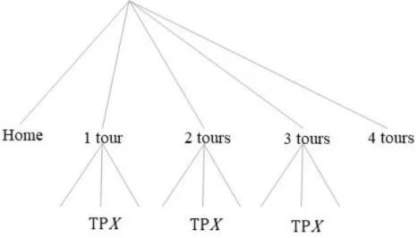
Figure 1 shows the nested logit model structure with number of tours conducted

during a day on the upper level and the specific tour pattern (TP) on the lower level.

The stay at home alternative (zero tours) and the four-tours pattern alternative lie

directly under the root in the logit tree and are not connected to the mode and

destination choice models2_{via a logsum, which is the case for one, two and three tours} patterns. Example of modelled tour patterns are:

1. Home-work-home (one tour)

2. Home-school-home, home-visit-home (two tours)

3. Home-school-home, home-visit-home, home-recreation-home (three tours)

The tour pattern is sensitive to order, i.e. the tour pattern home-visit-home followed by

home-school-home is different from the tour pattern number 2 above.

Figure 1: Nested logit model structure with number of tours on the upper level and tour patterns (TP) on the lower level.

2_{For a specification of the mode and destination choice models providing logsums as input to} the tour generation model see Kristoffersson et al. (2018).

(8)

5

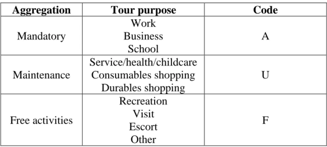
The number of alternatives in this kind of model can easily become very high.

Aggregation of tour purposes has therefore been conducted for some of the tour patterns

with two or three tours per day. The aggregation has been done according to Table 1.

After aggregation there are in total 86 alternatives in the model, out of which 1 is the

stay at home alternative, 10 are one tour patterns, 50 are two tours patterns, 24 are three

tours patterns and 1 is the four tours pattern (see appendix for detailed description of

which tour purposes are included in which alternative).

Table 1: Aggregation of tour purposes in the two and three tours patterns to reduce number of alternatives in the model.

Aggregation Tour purpose Code

Mandatory Work Business School A Maintenance Service/health/childcare Consumables shopping Durables shopping U Free activities Recreation Visit Escort Other F

The systematic components of the utility function (𝑣) are linear and have the form

shown in Equation 1.

𝑣(1) = 0

𝑣(2, … ,86) = 𝛼 + 𝛽𝑥

Equation 1

From Equation 1 it can be seen that the systematic component of the utility of staying at

home has been set to zero, whereas the systematic component of the other alternatives

are formulated as an alternative specific constant (𝛼) plus independent variables (𝑥)

with coefficients 𝛽 to be estimated. For some of the alternatives, only an alternative

(9)

6 2.2 Data

The model is estimated on data from the Swedish national travel survey in 2005-2006

(SIKA, 2007). Data consists of 26 949 observations and are from respondents of age

6-85, from the whole country and from different days and months of the year. The model

is estimated on tours shorter than 100 km, since this is a model for regional tour

generation.

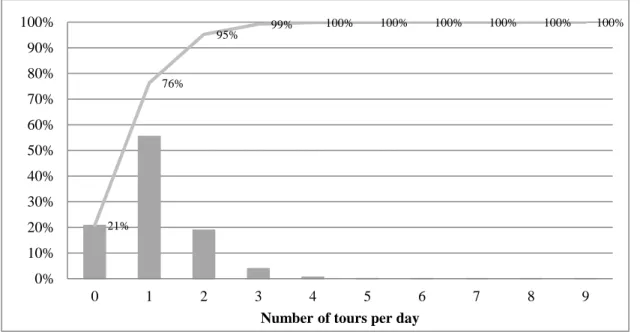
Figure 2 shows the percent of respondents in the survey that has conducted a

certain number of tours per day. From the figure it can be seen that only 5% of

respondents make three or more tours per day and that 21% of respondents stay at

home. The share of respondents staying at home are likely due to illness, taking care of

children, or similar, which is primarily not affected by changes in the transport system,

rather it could possibly be explained by demographical variables in the tour generation

model.

Figure 2: The distribution of respondents over different tour patterns in the data material.

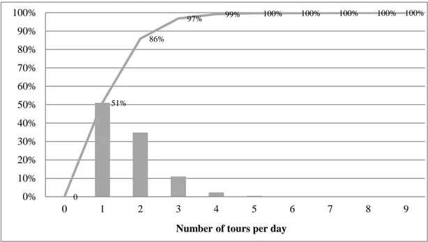
Even though only 5% of respondents make three tour patterns, these still account for

10% of total number of tours, see Figure 3. 21% 76% 95% 99% 100% 100% 100% 100% 100% 100% 0% 10% 20% 30% 40% 50% 60% 70% 80% 90% 100% 0 1 2 3 4 5 6 7 8 9

(10)

7

Figure 3:The distribution of tours over different tour patterns in the data material.

Figure 4 shows the distribution of tours over purposes for one, two and three tour

patterns. From the figure it can be seen that work is the most common purpose for one

tour patterns, whereas recreation is the most common purpose for two and three tour

patterns.

Figure 4: The distribution of tours over different purposes for one, two and three+ tour patterns. 0 51% 86% 97% 99% 100% 100% 100% 100% 100% 0% 10% 20% 30% 40% 50% 60% 70% 80% 90% 100% 0 1 2 3 4 5 6 7 8 9

Number of tours per day

0% 5% 10% 15% 20% 25% 30% 35% One tour Two tours Three+ tours

(11)

8 3. Results

3.1 Estimation results

The estimation of the model is conducted using the software Alogit (www.alogit.com ).

The estimation gives values on the coefficients 𝛽, but also on 𝛳, which are logit tree

parameters indicating the ratio of relative sensitivity of choices made at the upper level

(number of tours) and the lower level (tour patterns). The resulting values on 𝛳 are

given in Table 2. Values of 𝛳 should be between 0 and 1 in a nested logit model, which

is the case here.

Table 2: Estimation results for nested logit tree parameters.

Logit tree parameter (𝛳) Estimated parameter value t-value

𝛳_three (3 tours) 0.6735 9.0

𝛳_two (2 tours) 0.7584 21.9

𝛳_one (1 tour) 0.6946 26.6

The resulting values and t-statistics for the estimated parameters 𝛽 are given in

appendix due to the large number of utility functions. The main results are presented in

the following sections. When analysing and comparing the sign and size of the

estimated parameters, it is important to remember that that choices are made both

between different purposes within one, two and three tours patterns and between

(12)

9

Logsum from mode and destination choice model

The logsum variable (LS_purpose_nn3) from the mode and destination choice model has been included where significant. Logsums for all purposes included in the specific

tour pattern have been tested and the logsum contributing most to the explanatory power

have been included in the model.

The logsum is a good measure of accessibility. The estimation results for the

logsum are reasonable, with low sensitivity or not significant for trip purposes that are

mandatory such as work and school. These tours are made independently of the

accessibility to the work or school destination, given that you have a workplace or go to

school in a certain destination zone. The logsum is a more important variable for

flexible purposes such as for utility function number 39, where the logsum for the visit

purpose (LS_Visit_39) results in an estimated parameter value of 0.7285 with t-ratio

2.8, see Table 5.

Job status and Income

If the respondent has a job or not (Working_nn) is a strong variable in the model, e.g.

for utility function number 53 where a dummy for respondent is working (Working_53)

results in an estimated parameter value of 4.2 with t-ratio 4.1, see Table 5. Respondents

that are working have a higher probability of making more tours per day, this is

especially clear for the four tours pattern (e.g. variable Working_86 in Table 7 with

estimated parameter value 0.7599 and t-ratio 4.9).

3_{Here nn represents the utility function number. The variable is sometimes common to several} utility functions, in which case the span of utility functions is given by first and last utility function number as nnnn.

(13)

10

Income variables explain the possibility for respondents to participate in

activities that cost money. Income is also an indicator of part time work. Income

variables are in the model divided into very low income (I_Z_nn), low income

(I_L_nn), medium income (I_M_nn) and high income (I_H_nn). The range for what is

e.g. a high income varies across the utility functions. The exact definition for each case

is given in the parameter estimate tables in appendix. The results in Table 4 show that

high income reduces the probability of conducting tours with a cheap purpose such as

Visit (I_H_6, parameter value -0.5958, t-value 6.2), but increases the probability

substantially of making Business tours (I_H_4, parameter value 2.7470, t-ratio 6.4). A

very low income has a strong positive effect for Recreation as a one tour pattern (I_Z_7,

parameter value 0.3481, t-ratio 4.0), which is most likely interpreted as respondents not

working having a higher probability of making a Recreation tour as the only tour

pattern, rather than combined with Work in a two tours pattern.

Demography

The model includes demographic dummy variables for gender (Male_nn), age

(Age_yyyy_nn), presence of one or more children in the household (Child_nn), type of home (Villa_nn) and whether the respondent has access to both a drivers’ license and a car (Car_nn).

The results show that men participate to a smaller extent in maintenance tour

purposes such as Consumables shopping and Service/health/childcare (e.g. Male_5,

parameter value -0.2223, t-ratio -2.4). Age is of course important for the generation of

school tours, but age above 65 also increases the probability of making an SHC tour

(Age_65yy_5, parameter value 0.3543, t-ratio3.5). Children in the household has a

(14)

11

1.0760, t-ratio 7.8), Service/Health/Childcare tours (e.g. Child_29, parameter value

1.899, t-ratio 6.3) and generation of four tours patterns (Child_86, parameter value

0,6786, t-ratio 5.4).Access to car and drivers’ licence has a strong positive effect on generation of Escort tours (e.g. Car_8, parameter value 1.3020, t-ratio 7.6) and on

generation of four tours patterns (Car_86, parameter value 0,8777, t-ratio 4.9).

Weekend and season

Weekend and seasonal effects are strong in the estimated tour generation model. These

variables are included to be able to use the model for studies of how tour generation

varies across the year and week. Typically, Recreational and Visit tour patterns increase

during weekends, summer and Christmas holidays, whereas Work, School and Business

tour patterns decrease during these time periods (e.g. JA_7, parameter value 0.3823,

t-ratio 5.2 and WE_2, parameter value -2.5580, t-t-ratio -34.2). Consumables and Durables

shopping is typically conducted on Saturdays (e.g. Sat_9, parameter value 0.6203,

t-ratio 8.2).

3.2 Validation against data

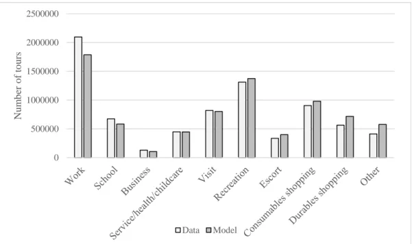
Figure 5 shows number of tours per purpose generated by the model and compared to

the data it was estimated on. The numbers represent yearly averages per day. Number of

work tours are lower in the model compared to data since tours implying lunch at home

were redefined from two work tours to one work tour, as there should not be a

(15)

12

Figure 5: Number of tours per purpose for model application compared to survey data (yearly average per day).

3.3 Simulated effects of changes to input data

An important issue is how the model reacts on increases in income. Simulations have

been made of increases in income by keeping the share of respondents with zero income

constant and spread out the income increase evenly among the other income groups.

Tests have been made with 10 % and 50 % increase in income. The simulations are

partial in the sense that only the tour generation model has been run, i.e. no changes

have been made to car ownership and logsums from the mode and destination choice

model.

The result of the 10 % income increase is an increase in number of tours by 0,04%

and the 50% income increase results in a 0,3% increase in number of tours. The largest

effect is that the four tours patterns increase. The tour purpose that increase the most is

Business tours. Visit and Consumables shopping decrease when incomes are increased

in the model. The net effect of partially increasing income in the tour generation model

is thus close to zero when it comes to generation of tours.

0 500000 1000000 1500000 2000000 2500000 Nu m b er o f to u rs Data Model

(16)

13 4. Conclusions

In this paper, a new type of tour generation model has been estimated, which extends

the conventional generation model by including the daily tour pattern in the estimation.

This new model type introduces a soft upper limit to the number of tours conducted by

each traveller per day.

Result of the estimation shows that access to car and drivers’ licence, having a job and presence of children in the household increases the probability of making many

tours per day. Furthermore, the results show that weekend and holiday season are

important determinants of when different tour purposes are generated, and that

accessibility (the logsum from the mode and destination choice model) is an important

variable for non-mandatory tour purposes such as recreation, but not for mandatory

purposes such as school tours. Age is an important variable for school tours and for

service tours for elderly. High income increases the probability of conducting business

tours as well as tour patterns that include expensive activities such as shopping. On the

other hand, high income reduces the probability of conducting cheap activities such as

visiting friends and family.

One important aspect of a tour generation model is to what extent number of

tours increases with changes in income. Test have been made with increasing the

income in the model while keeping car ownership and logsums constant. These test

show very small increases in number of tours as income increases. The total effect in a

future application of the model to a forecast year is difficult to assess, but the tests

indicate that the model does not give an unrealistic response to income increases.

Population increase is the dominating driving force of traffic growth in Sweden, as well

(17)

14

population is growing in the cities or on the country-side.

Acknowledgement

This research was performed within the project ‘Sampers4’ supported by The Swedish

Transport Administration under Grant TRV 2017/86915. We are grateful to Daniel

Jonsson (KTH Royal Institute of Technology) and Leonid Engelson (The Swedish

Transport Administration) for giving comments on earlier versions of this work.

References

Agyemang-Duah, K., Anderson, W. P., & Hall, F. L. (1995). Trip generation for shopping travel. Transportation Research Record, (1493).

Ben-Akiva, M., & Lerman, S. (1985). Discrete choice analysis: theory and application

to travel demand (Vol. 9). The MIT Press.

Beser, M., & Algers, S. (2002). SAMPERS—The new Swedish national travel demand forecasting tool. In National Transport Models (pp. 101–118). Springer.

Retrieved from http://link.springer.com/10.1007/978-3-662-04853-5_9

Bradley, M., Bowman, J. L., & Griesenbeck, B. (2010). SACSIM: An applied activity-based model system with fine-level spatial and temporal resolution. Journal of

Choice Modelling, 3(1), 5–31.

Broadstock, D. C., Collins, A., & Hunt, L. C. (2010). Modelling car trip generations for UK residential developments using data from TRICS. Transportation Planning

and Technology, 33(8), 671–678.

City of Stockholm. (2010). Analys av flöden i Stockholmstrafiken. Utveckling och

nuläge 2009 (Analysis of traffic flows in Stockholm. Development and current situation 2009). Retrieved from

https://insynsverige.se/documentHandler.ashx?did=105275

Cubukcu, K. M. (2001). Factors affecting shopping trip generation rates in metropolitan areas. Studies in Regional and Urban Planning, 9, 51–68.

Ewing, R., DeAnna, M., & Li, S.-C. (1996). Land use impacts on trip generation rates.

Transportation Research Record: Journal of the Transportation Research Board, (1518), 1–6.

(18)

15

Frank, L. D. (1996). An analysis of relationships between urban form (density, mix, and jobs: housing balance) and travel behavior (mode choice, trip generation, trip length, and travel time). Transportation Research Part A, 1(30), 76–77.

Frank, L., Kerr, J., Chapman, J., & Sallis, J. (2007). Urban form relationships with walk trip frequency and distance among youth. American Journal of Health

Promotion, 21(4_suppl), 305–311.

Gunn, H. (1994). The Netherlands National Model: a review of seven years of

application. International Transactions in Operational Research, 1(2), 125–133. Retrieved from

http://www.sciencedirect.com/science/article/pii/0969601694900140

Kristoffersson, I., Daly, A., & Algers, S. (2018). Modelling the attraction of travel to shopping destinations in large-scale modelling. Transport Policy, 68, 52–62. Molla, M. M., Stone, M. L., & Motuba, D. (2017). Developing an activity-based trip generation model for small/medium size planning agencies. Transportation

Planning and Technology, 40(5), 540–555.

Ortuzar, J., & Willumsen, L. (1994). Modelling transport. Wiley, New York. Pinjari, A. R., & Bhat, C. R. (2011). Activity-based travel demand analysis. In A

Handbook of Transport Economics. Edward Elgar Publishing.

SIKA. (2007). RES 2005–2006 Den nationella resvaneundersökningen (No. 2007:19). Retrieved from

https://www.trafa.se/globalassets/sika/sika-statistik/ss_2007_19_1.pdf?_t_id=1B2M2Y8AsgTpgAmY7PhCfg%3d%3d&_t_ q=res+2005-2006&_t_tags=language%3asv%2csiteid%3af9e4ecf2-4fe2-49ec- bd2f-7b6540d3eb17&_t_ip=213.113.174.187&_t_hit.id=Knowit_EPi_Site_Trafa_Kit Modules_Document_Models_Media_DocumentFile/_7ea2d76e-3be7-4f9a-a419-5b7ebacbaa8d&_t_hit.pos=2

Trafikverket. (2018). Samhällsekonomisk kalkyl av höghastighetsjärnväg 250 km/h

(Cost-benefit analysis of high speed rail 250 km/h) (No. 2014/54842). Retrieved

from

https://www.trafikverket.se/TrvSeFiler/Foretag/Planera_o_utreda/Samhallsekon omiskt_beslutsunderlag/Regionoverskridande/3.%20Investering/JTR1801%20oc

(19)

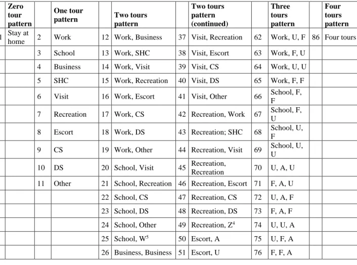
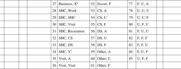
16 Appendix

In this appendix, tables are given that show which tour purposes are included in which utility function (Table 3), the estimated parameters for one, two, three and four tours patterns (Table 4 - Table 7) and the alternative specific constants for one, two and three tours patterns (

Table 8 - Table 10).

There are some combined alternatives, indicated W, X, Y and Z, in the table below. The

combined alternatives are split into travel purposes based on shares derived from the

travel survey used for the model estimation.

Table 3: Utility function numbers and the tour purposes they encompass. Zero

tour pattern

One tour

pattern Two tours pattern Two tours pattern (continued) Three tours pattern Four tours pattern 1 Stay at

home 2 Work 12 Work, Business 37 Visit, Recreation 62 Work, U, F 86 Four tours

3 School 13 Work, SHC 38 Visit, Escort 63 Work, F, U

4 Business 14 Work, Visit 39 Visit, CS 64 Work, U, U

5 SHC 15 Work, Recreation 40 Visit, DS 65 Work, F, F

6 Visit 16 Work, Escort 41 Visit, Other 66 School, F,

F

7 Recreation 17 Work, CS 42 Recreation, Work 67 School, F,

U

8 Escort 18 Work, DS 43 Recreation; SHC 68 School, U,

F

9 CS 19 Work, Other 44 Recreation, Visit 69 School, U,

U

10 DS 20 School, Visit 45 Recreation,

Recreation 70 U, A, U

11 Other 21 School, Recreation 46 Recreation, Escort 71 F, A, U

22 School, CS 47 Recreation, CS 72 U, A, F

23 School, DS 48 Recreation, DS 73 F, A, F

24 School, Other 49 Recreation, Z4 ₇₄ _{U, U, A}

25 School, W5 _{50 Escort, A} ₇₅ _{U, F, A}

26 Business, Business 51 Escort, U 76 F, F, A

4_{Combination of School, Business and Other} 5_{Combination of Work, Business, SHC and Escort}

(20)

17 27 Business, X6 _{52 Escort, F} ₇₇ _{F, U, A} 28 SHC, Work 53 CS, A 78 U, U, U 29 SHC, SHC 54 CS, U 79 U, U, F 30 SHC, Visit 55 CS, F 80 U, F, U 31 SHC, Recreation 56 DS, A 81 F, U, U 32 SHC, CS 57 DS, U 82 F, F, F 33 SHC, DS 58 DS, F 83 F, F, U 34 SHC, Y7 _{59 Other, A} ₈₄ _{F, U, F} 35 Visit, A 60 Other, U 85 U, F, F

36 Visit, Visit 61 Other, F

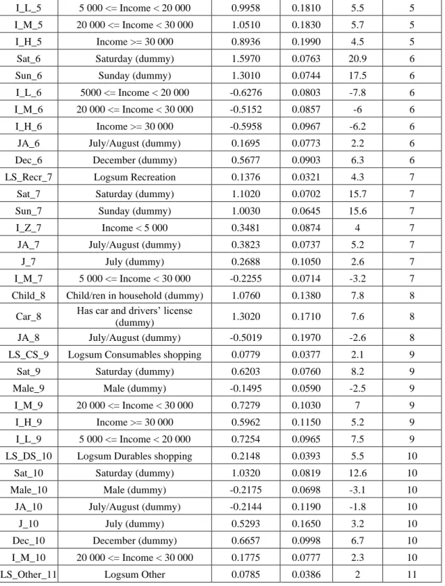
Table 4: Resulting parameter estimates for one tour patterns. The number at the end of each parameter name indicates the corresponding utility function number (see Table 3). Income is given in Euro, converted from Swedish currency using the conversion rate 10 SEK = 1 EUR.

Name Description Estimate Std. Error T-Ratio Utility function

C1 Alternative specific constant

common to all one tour patterns 0.4746 0.179 2.6 2-11

LS_work_2 Logsum work tours 0.0926 0.0225 4.1 2

WE_2 Weekend (dummy) -2.5580 0.0748 -34.2 2

I_H_2 Income > 20 000 0.2377 0.0653 3.6 2

JA_2 July/August (dummy) -0.4938 0.0756 -6.5 2

J_2 July (dummy) -0.7029 0.1300 -5.4 2

Age_0616_3 Age 6-15 (dummy) 4.1430 0.1360 30.4 3

Age_1619_3 Age 16-16 (dummy) 3.6720 0.1460 25.1 3

Age_1925_3 Age 20-25 (dummy) 2.3310 0.1590 14.7 3

Age_2535_3 Age 26-36 (dummy) 1.1920 0.1760 6.8 3

Villa_3 Live in one-family house (dummy) -0.3406 0.0681 -5 3

J_3 July (dummy) -3.1800 0.7210 -4.4 3

I_H_4 Income > 30 000 2.7470 0.4330 6.4 4

I_L_4 5000 <= Income < 20 000 1.4140 0.4340 3.3 4

I_M_4 20 000 <= Income < 30 000 2.3040 0.4310 5.4 4

NS_4 Northern Sweden (dummy) -0.9426 0.1470 -6.4 4

WE_4 Weekend (dummy) -1.5250 0.2010 -7.6 4

Male_5 Male (dummy) -0.2223 0.0946 -2.4 5

Age_65yy_5 Age 65 or more (dummy) 0.3543 0.1010 3.5 5

6_{Combination of Work, SHC, Visit, Recreation, Escort, CS, DS and Other} 7_{Combination of School, Business, Escort and Other}

(21)

18

I_L_5 5 000 <= Income < 20 000 0.9958 0.1810 5.5 5

I_M_5 20 000 <= Income < 30 000 1.0510 0.1830 5.7 5

I_H_5 Income >= 30 000 0.8936 0.1990 4.5 5

Sat_6 Saturday (dummy) 1.5970 0.0763 20.9 6

Sun_6 Sunday (dummy) 1.3010 0.0744 17.5 6

I_L_6 5000 <= Income < 20 000 -0.6276 0.0803 -7.8 6

I_M_6 20 000 <= Income < 30 000 -0.5152 0.0857 -6 6

I_H_6 Income >= 30 000 -0.5958 0.0967 -6.2 6

JA_6 July/August (dummy) 0.1695 0.0773 2.2 6

Dec_6 December (dummy) 0.5677 0.0903 6.3 6

LS_Recr_7 Logsum Recreation 0.1376 0.0321 4.3 7

Sun_7 Sunday (dummy) 1.0030 0.0645 15.6 7

I_Z_7 Income < 5 000 0.3481 0.0874 4 7

JA_7 July/August (dummy) 0.3823 0.0737 5.2 7

J_7 July (dummy) 0.2688 0.1050 2.6 7

I_M_7 5 000 <= Income < 30 000 -0.2255 0.0714 -3.2 7

Child_8 Child/ren in household (dummy) 1.0760 0.1380 7.8 8

Car_8 Has car and drivers’ license

(dummy) 1.3020 0.1710 7.6 8

LS_CS_9 Logsum Consumables shopping 0.0779 0.0377 2.1 9

Male_9 Male (dummy) -0.1495 0.0590 -2.5 9

I_M_9 20 000 <= Income < 30 000 0.7279 0.1030 7 9

I_H_9 Income >= 30 000 0.5962 0.1150 5.2 9

I_L_9 5 000 <= Income < 20 000 0.7254 0.0965 7.5 9

LS_DS_10 Logsum Durables shopping 0.2148 0.0393 5.5 10

Male_10 Male (dummy) -0.2175 0.0698 -3.1 10

J_10 July (dummy) 0.5293 0.1650 3.2 10

I_M_10 20 000 <= Income < 30 000 0.1775 0.0777 2.3 10

LS_Other_11 Logsum Other 0.0785 0.0386 2 11

Table 5: Resulting parameter estimates for two tours patterns. The number at the end of each parameter name indicates the corresponding utility function number (see Table 3). Income is given in Euro, converted from Swedish currency using the conversion rate 10 SEK = 1 EUR.

Name Description Estimate Std.

Error T-Ratio

Utility function

common to all two tours patterns -5.605 0.328 -17.1 12-61

(22)

19

LS_Work_12 Logsum Work tour 0.1118 3.29E-02 3.4 12-19

WE_1319 Weekend (dummy) -2.742 0.143 -19.1 13-19

I_H_14 Income >= 30 000 -0.3298 0.147 -2.2 14

(dummy) 2.001 0.588 3.4 16

LS_CS_17 Logsum Consumables shopping 0.1704 9.38E-02 1.8 17

I_M_19 200 000 <= Income < 30 000 0.4982 0.24 2.1 19

Age_0616_20 Age 6-15 (dummy) 3.561 0.289 12.3 20

Age_0619_20 Age 16-19 (dummy) 3.675 0.307 12 20

Age_0616_21 Age 6-15 (dummy) 3.377 0.211 16 21

Age_1619_21 Age 16-19 (dummy) 2.906 0.233 12.5 21

I_M_21 Income >= 5 000 -0.6133 0.159 -3.8 21

Age_20yy_22 Age 20 or more (dummy) -2.257 0.271 -8.3 22

Villa_22 Lives in one-family house (dummy) -0.9483 0.247 -3.8 22

Age_1619_23 Age 16-19 (dummy) -0.998 0.387 -2.6 23

JA_23 July/August (dummy) -1.315 0.435 -3 23

Age_1619_25 Age 16-19 (dummy) 0.8737 0.39 2.2 25

I_L_27 5 000 <= Income < 20 000 -1.147 0.317 -3.6 27

(dummy) 1.952 0.398 4.9 27

WE_28 Weekend (dummy) -1.769 0.612 -2.9 28

Male_29 Male (dummy) -0.871 0.295 -2.9 29

I_L_29 5 000 <= Income < 20 000 1.024 0.264 3.9 29

LS_SHC_31 Logsum SHC 0.4322 9.73E-02 4.4 31

Male_31 Male (dummy) -0.5885 0.316 -1.9 31

I_H_32 Income >= 30 000 0.5407 0.324 1.7 32

Male_34 Male (dummy) -1.266 0.38 -3.3 34

Working_35 Has a job (dummy) 2.378 0.77 3.1 35

WE_3641 Weekend (dummy) 1.267 0.137 9.3 36-41

LS_Visit_39 Logsum Visit 0.7285 0.261 2.8 39

Age_2025_42 Age 20-25 (dummy) 1.417 0.374 3.8 42

(23)

20

LS_Recr_4249 Logsum Recreation 0.1314 5.33E-02 2.5 42-49

Age_0019_44 Age 0-19 (dummy) 1.468 0.185 7.9 44

WE_44 Weekend (dummy) 1.929 0.19 10.2 44

Age_0019_45 Age 0-19 (dummy) 1.017 0.17 6 45

WE_45 Weekend (dummy) 1.481 0.156 9.5 45

WE_46 Weekend (dummy) 1.114 0.337 3.3 46

WE_47 Weekend (dummy) 0.9468 0.24 4 47

WE_48 Weekend (dummy) 0.9223 0.286 3.2 48

WE_49 Weekend (dummy) 1.631 0.44 3.7 49

LS_Escort_50 Logsum Escort 0.6222 0.256 2.4 50

I_Z_50 Income <= 5 000 -1.831 1.06 -1.7 50

I_Z_51 Income <= 5 000 -1.257 0.489 -2.6 51

(dummy) 1.855 0.384 4.8 52

LS_CS_52 Logsum Consumables shopping 0.333 0.167 2 52

WE_54 Weekend (dummy) 0.5637 0.167 3.4 54

Age_65yy_54 Age 65 or more (dummy) 0.4777 0.173 2.8 54

LS_CS_54 Logsum Consumables shopping 0.4681 0.107 4.4 54

WE_55 Weekend (dummy) 0.8087 0.135 6 55

LS_CS_55 Logsum Consumables shopping 0.2275 8.46E-02 2.7 55

I_Z_55 Income <= 5 000 -0.4165 0.196 -2.1 55

J_55 July (dummy) 0.5821 0.212 2.7 55

Male_55 Male (dummy) -0.3014 0.132 -2.3 55

Male_56 Male (dummy) -0.8593 0.454 -1.9 56

WE_56 Weekend (dummy) -1.374 0.624 -2.2 56

LS_DS_57 Logsum Durables shopping 0.427 0.11 3.9 57

LS_DS_58 Logsum Durables shopping 0.3304 8.29E-02 4 58

J_58 July (dummy) 0.5218 0.239 2.2 58

Male_59 Male (dummy) -0.9143 0.533 -1.7 59

WE_60 Weekend (dummy) 0.5147 0.181 2.8 60

LS_CS_60 Logsum Consumables shopping 0.3349 0.112 3 60

Sun_61 Sunday (dummy) 0.6839 0.219 3.1 61

(24)

21

Table 6: Resulting parameter estimates for three tours patterns. The number at the end of each parameter name indicates the corresponding utility function number (see Table 3).

Name Description Estimate Std. Error T-Ratio Utility function

common to all three tours patterns -5.525 0.78 -7.1 62-85

WE_6265 Weekend (dummy) -2.953 0.429 -6.9 62-65

LS_Work_6265 Logsum Work 0.148 8.33E-02 1.8 62-65

JA_6264 July/August (dummy) 0.4954 0.23 2.2 62-64

Age_0019_65 Age 0-19 (dummy) 1.651 0.689 2.4 65

Age_0616_66 Age 6-15 (dummy) 3.662 0.613 6 66

Age_1619_66 Age 16-19 (dummy) 3.127 0.685 4.6 66

Age_1931_66 Age 20-25 (dummy) 1.886 0.828 2.3 66

JA_6669 July/August (dummy) -1.219 0.394 -3.1 66-69

Age_0616_67 Age 6-15 (dummy) 2.689 0.809 3.3 67

Age_1619_67 Age 16-19 (dummy) 2.17 1.01 2.1 67

Age_0616_68 Age 6-15 (dummy) 3.046 0.558 5.5 68

Age_1619_68 Age 16-19 (dummy) 2.17 0.724 3 68

Age_0616_69 Age 6-15 (dummy) 1.362 0.615 2.2 69

WE_7077 Weekend (dummy) -1.473 0.375 -3.9 70-77

LS_SHC_7885 Logsum SHC 0.8138 0.105 7.8 78-85

WE_79 Weekend (dummy) 0.3949 0.228 1.7 79

WE_82 Weekend (dummy) 1.249 0.221 5.6 82

J_83 July (dummy) 1.953 0.437 4.5 83

WE_85 Weekend (dummy) 0.8765 0.231 3.8 85

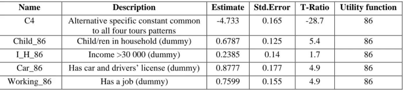
Table 7: Resulting parameter estimates for four tours patterns. The number at the end of each parameter name indicates the corresponding utility function number (see Table 3). Income is given in Euro, converted from Swedish currency using the conversion rate 10 SEK = 1 EUR.

Name Description Estimate Std.Error T-Ratio Utility function

C4 Alternative specific constant common

to all four tours patterns

-4.733 0.165 -28.7 86

I_H_86 Income >30 000 (dummy) 0.2385 0.14 1.7 86

Car_86 Has car and drivers’ license (dummy) 0.8777 0.177 4.9 86

Table 8: Resulting estimates of alternative specific constants for one tour patterns. Utility function number 2 is the reference alternative.

ASC Estimate Std. Error T-Ratio

asc3 -3.659 0.22 -16.6

asc4 -4.740 0.465 -10.2

(25)

22 asc6 -2.282 0.189 -12.1 asc7 -3.197 0.311 -10.3 asc8 -5.110 0.252 -20.3 asc9 -3.028 0.273 -11.1 asc10 -3.944 0.292 -13.5 asc11 -3.146 0.276 -11.4

Table 9: Resulting estimates of alternative specific constants for two tours patterns. Utility function number 12 is the reference alternative.

ASC Estimate Std. Error

T-Ratio ASC Estimate Std. Error T-Ratio asc13 1.008 0.271 3.7 asc38 -1.416 0.426 -3.3 asc14 2.747 0.209 13.1 asc39 -5.768 1.93 -3 asc15 3.225 0.199 16.2 asc40 -0.964 0.395 -2.4 asc16 -0.355 0.617 -0.6 asc41 -0.877 0.39 -2.2 asc17 1.775 0.61 2.9 asc42 -0.077 0.556 -0.1 asc18 1.942 0.214 9.1 asc43 -1.209 0.543 -2.2 asc19 1.211 0.262 4.6 asc44 -0.925 0.543 -1.7 asc20 -0.018 0.421 0 asc45 -0.178 0.53 -0.3 asc21 1.460 0.387 3.8 asc46 -1.395 0.563 -2.5 asc22 3.001 0.383 7.8 asc47 -0.617 0.534 -1.2 asc23 2.705 0.36 7.5 asc48 -0.970 0.545 -1.8 asc24 1.581 0.377 4.2 asc49 -2.149 0.619 -3.5 asc25 0.864 0.361 2.4 asc50 -4.521 1.32 -3.4 asc26 -0.494 0.391 -1.3 asc51 -0.320 0.415 -0.8 asc27 -0.427 0.501 -0.9 asc52 -2.718 0.982 -2.8 asc28 -1.525 0.655 -2.3 asc53 -3.127 1.05 -3 asc29 -2.112 0.585 -3.6 asc54 -1.496 0.724 -2.1 asc30 -1.660 0.52 -3.2 asc55 0.533 0.591 0.9 asc31 -1.146 0.517 -2.2 asc56 -0.638 0.304 -2.1 asc32 -1.469 0.515 -2.9 asc57 -0.796 0.391 -2 asc33 -1.928 0.529 -3.6 asc58 -0.676 0.62 -1.1 asc34 -1.044 0.513 -2 asc59 -2.111 0.789 -2.7 asc35 -2.434 0.778 -3.1 asc60 -0.728 0.736 -1 asc36 0.270 0.353 0.8 asc61 -0.009 0.623 0 asc37 0.150 0.354 0.4

Table 10: Resulting estimates of alternative specific constants for three tours patterns. Utility function number 62 is the reference alternative.

ASC Estimate Std. Error T-Ratio

asc63 -1.130 0.251 -4.5

asc64 -0.773 0.221 -3.5

asc65 -0.187 0.202 -0.9

(26)

23 asc67 -2.973 0.981 -3 asc68 -2.279 0.844 -2.7 asc69 -1.982 0.793 -2.5 asc70 -1.049 0.779 -1.3 asc71 -1.608 0.845 -1.9 asc72 -0.692 0.751 -0.9 asc73 -0.797 0.758 -1.1 asc74 -0.222 0.725 -0.3 asc75 -1.896 0.893 -2.1 asc76 -1.049 0.779 -1.3 asc77 -2.413 1.21 -2 asc78 -3.053 0.783 -3.9 asc79 -3.276 0.788 -4.2 asc80 -4.181 0.796 -5.3 asc81 -1.123 0.704 -1.6 asc82 -0.473 0.697 -0.7 asc83 -4.627 0.809 -5.7 asc84 -3.583 0.788 -4.5 asc85 -3.575 0.792 -4.5