This is the published version of a paper published in Metals.
Citation for the original published paper (version of record):
Matsushita, T., Ghassemali, E., Saro, A., Elmquist, L., Jarfors, A. (2015) On Thermal Expansion and Density of CGI and SGI Cast Irons. Metals, 5(2): 1000-1019
http://dx.doi.org/10.3390/met5021000
Access to the published version may require subscription. N.B. When citing this work, cite the original published paper.
Permanent link to this version:
metals
ISSN 2075-4701www.mdpi.com/journal/metals/ Article
On Thermal Expansion and Density of CGI and SGI Cast Irons
Taishi Matsushita *, Ehsan Ghassemali †, Albano Gómez Saro †, Lennart Elmquist and Anders E. W. Jarfors †
Department of Materials and Manufacturing, School of Engineering, Jönköping University, P.O. Box 1026, Jönköping SE-551 11, Sweden; E-Mails: ehsan.ghassemali@jth.hj.se (E.G.); albanogs@hotmail.com (A.G.S.); lennart.elmquist@jth.hj.se (L.E.);
anders.jarfors@jth.hj.se (A.E.W.J.)
† These authors contributed equally to this work.
* Author to whom correspondence should be addressed; E-Mail: taishi.matsushita@jth.hj.se;
Tel.: +46-36-101697; Fax: +46-36-166560. Academic Editor: Hugo F. Lopez
Received: 30 April 2015 / Accepted: 26 May 2015 / Published: 4 June 2015
Abstract: The thermal expansion and density of Compacted Graphite Iron (CGI) and
Spheroidal Graphite Iron (SGI) were measured in the temperature range of 25–500 °C using push-rod type dilatometer. The coefficient of the thermal expansion (CTE) of cast iron can be expressed by the following equation: CTE = 1.38 × 10⁻⁵ + 5.38 × 10⁻⁸ N − 5.85 × 10⁻⁷ G + 1.85 × 10⁻⁸ T − 2.41 × 10⁻⁶ RP/F − 1.28 × 10⁻⁸ NG − 2.97 × 10⁻⁷ GRP/F + 4.65 × 10⁻⁹ TRP/F + 1.08 × 10⁻⁷ G2 − 4.80 × 10⁻¹¹ T2 (N: Nodularity, G: Area fraction of graphite (%), T: Temperature (°C), RP/F: Pearlite/Ferrite ratio in the matrix).
Keywords: thermal expansion; high-silicon cast iron; dilatometer; density; cycle test
1. Introduction
The development and use of high performance powertrain components is crucial for the performance of different vehicles. In order to meet the demands for more efficient transport solutions involving improved energy conversion efficiency in engines as well as lighter components and systems for overall enhanced performance, lighter and/or stronger materials are an important means.
Key materials for engine components (such as engine blocks, cylinder heads, etc.) include various cast materials such as cast irons of different grades as well as light metals as aluminum. For heavy truck diesel engines, current and future expected solutions are based on cast irons. For car engines, aluminum is often combined with other metals, as in the case of cast aluminum engine block with cast iron cylinder liners. Legislation and needs for lower emissions and improved efficiency mean higher pressures and temperatures and thus increasing demands on material performance in both cases. Moreover, the downsizing of engines with preserved demands on performance adds to this scenario. To meet these requirements, it is important to investigate factors necessary to create conditions for closer tolerances and optimization of mechanical and thermal properties by control of graphite morphology.
The idea of near net shape is to explore the possibility of designing and casting components with better tolerance and more accurate dimensions to decrease manufacturing cost and required machining. To develop a robust casting process is a prerequisite to cast more accurately. Compacted graphite iron (CGI) has become an interest of the automotive industry [1]. Compacted graphite cast iron is considered more difficult than for grey iron, hence it is interesting to cast with minimal processing requirements. The current project focuses on the casting itself and includes both simulation and verification through field trials.
A possibility to reduce the variations in matrix hardness is to use a material with higher Si content to create a solid solution strengthened ferritic matrix instead [2]. As the solution strengthening effect is achieved by an increased Si-content, this also reduces the carbides as Si is known to reduce tendency for carbide formation in cast irons. For solution strengthened ductile iron a number of interesting properties are obtained, and the existing requirements for mechanical properties fulfilled (similar to a matrix consisting of 50% ferrite and 50% perlite). However, for the same UTS, silicon solution strengthened iron shows higher ductility compared to the one with 50% pearlite. Furthermore, the obtained hardness is uniform and usually falls within ±5 HBW. The same approach can also be applied to compacted graphite iron material with increased Si content, yielding UTS of 565 MPa, elongation of 10% and hardness of 207 HBW. For CGI materials SinterCast has obtained one patent for solution hardening [3].
For the matrix, both Carbon and Silicon will have solution hardening contributions where size differences and effective change in the shear modulus are direct factors for the effectiveness of the alloying [4]. Elements such as silicon and carbon are also strongly coupled thermodynamically adding to the difficulty of finding an optimum. This also results because there is a strong influence from other elements such as Vanadium [5].
The research focus will be on how the additions of elements responsible for solution hardening affect nucleation and growth and to what extent nucleation is affected by venturing outside the conventional concentration range for CGI materials. For graphite morphology, Sulfur and Oxygen influence nodularity as does Magnesium [6]. Similarly solidification rate too has a significant effect.
Therefore, the current project is focused on Si-alloyed compacted graphite iron, to enable use of Si-alloyed CGI with potentially more robust manufacturing and better casting properties for engines components. Interaction of Si within CGI material is very complex and not fully understood. Some studies suggest that Si-alloyed compacted graphite iron does not meet the requirements imposed on the material. Among other things, lower thermal conductivity has been highlighted and excessive Si content can affect the machinability [7]. The conclusion is that more research is needed to clarify
the Si-alloyed CGI capability, involving casting of samples and examination of mechanical properties, machinability and thermal conductivity.
The current work addresses the aspect of thermal properties and mechanical behavior. As temperature in engine applications requires both the understanding of thermal expansion and the effect of thermal cycling on thermal expansion both aspects are currently addressed for both ferritic-perlitic materials and for fully ferritic materials with different graphite morphology.
2. Experimental
2.1. Materials
The chemical compositions of different cast iron supplied in the present study are given in Table 1.
Table 1. Chemical compositions of the different cast iron (mass %).
Elements SGI-1 SGI-2 SGI-3 CGI-1 CGI-2
C 3.28 3.13 3.51 3.24 3.18 Si 3.73 4.25 2.36 3.44 3.87 Mn 0.169 0.169 0.408 0.17 0.167 P 0.009 0.0095 0.0063 0.0069 0.0072 S 0.0056 0.0065 0.0043 0.0062 0.0072 Cr 0.028 0.029 0.025 0.028 0.028 Ni 0.045 0.041 0.039 0.048 0.047 Mo 0.0012 0.0016 0.0028 0.0034 0.0037 Mg 0.037 0.036 0.036 0.0061 0.0062
Fe Balance Balance Balance Balance Balance
CE 1 4.53 4.55 4.30 4.39 4.47
1 CE: Carbon Equivalent = C% + (Si% + P%)/3.
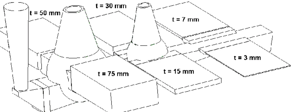
The samples for the thermal expansion measurement were taken from a cast component shown in Figure 1, from different thickness (t). In the present study, the samples from following plates were used: SGI-1 (t = 50 mm); SGI-2 (t = 15, 50 and 75 mm); SGI-3 (t = 15, 50 and 75 mm); CGI-1 (t = 50 mm); and CGI-2 (t = 15, 50 and 75 mm).
The thinner plate is corresponding to the faster cooling rate during the casting and the microstructure will be changed accordingly.
2.2. Dilatometry
Thermal expansion measurements were carried out from room temperature to 500 °C during heating cycle at the rate of 5 K/min using a Netzsch DIL 402 C push-rod dilatometer (Selb, Germany). The experimental apparatus consisted of a heating chamber, a displacement transducer, a digital system for logging (computer) and a push-rod.
The samples subjected for thermal cycling were heated and cooled 46 times between 55 °C and 600 °C with 10 K/min. The heating rate and maximum temperature were slightly changed with single cycle tests due to the limitation of experimental apparatus.
An alumina standard sample (6 mm in diameter × 12 mm in length) was used for the baseline measurement. The cast iron samples were cut into cylindrical pieces (6 mm in diameter × 12 mm in length). The sample was cleaned with acetone before experiments. After the sample was placed in the chamber, the chamber was flushed three times by helium. The temperature was measured with a Type S thermocouple set beside the sample. The temperature and change in length were recorded in the computer. The coefficient of thermal expansion (CTE) was obtained from the slope of ΔL/LX0 (where ΔL: change in length and LX0: initial length) against temperature. The details of the analysis method are described in Appendix A.
2.3. Microstructural Characterization
In many cases, the thermophysical properties of cast irons are influenced by microstructures such as nodularity, graphite amount and pearlite/ferrite ratio. The microstructure of the component will be influenced by the cooling rate during the casting. As mentioned in the Experimental section, the samples were taken from t = 15, 50 and 75 mm parts in this study to investigate the influence of the microstructure. The nodularity and graphite amount of each sample were measured using optical microscope Leica Leitz DMRX (Wetzlar, Germany) with Leica Q-Win v3 software (Wetzlar, Germany). The magnification was 100×. Minimum length of graphite was set as 10 μm for nodularity measurement. Forty pictures were taken for each sample to cover an area larger than 10 mm2. The nodularity was measured with the following equation (ISO standard method [8]).
Graphite (ISO form VI) Graphite (ISO form IV + V)
Graphite (All) 0.5 Nodularity (%) 100% A A A
(1)where AGraphite (IOS form VI): the surface area of graphite with roundness higher than 0.625 (ISO 945 form VI); AGraphite (ISO form IV+V): the surface area of graphite with roundness between 0.525 and 0.625 (ISO 945 form IV and V); and AGraphite (All): the surface area of all graphite.
3. Results and Discussion
3.1. Microstructure
The measured nodularity, graphite amount and ferrite/perlite amount are summarized in Tables 2 and 3, respectively. The amount of graphite in Table 3 represents the area fraction of graphite.
Table 2. Nodularity (%) of samples.
Thickness (mm) SGI-1 SGI-2 SGI-3 CGI-1 CGI-2
15 - 30.7 75.4 - 17.0
50 66.4 55.6 74.9 15.7 7.33
75 - 53.7 82.6 - 3.92
Table 3. Graphite and ferrite/perlite area fractions (%).
Samples Graphite ASTM Ferrite ASTM Pearlite
SGI-3, 15 mm 3.40 33.96 62.64 SGI-3, 50 mm 7.84 38.60 53.56 SGI-3, 75 mm 8.80 38.67 52.53 SGI-1, 50 mm 9.05 90.95 0 SGI-2, 15 mm 2.12 97.88 0 SGI-2, 50 mm 6.78 93.22 0 SGI-2, 75 mm 5.57 94.43 0 CGI-1, 50 mm 6.09 93.91 0 CGI-2, 15 mm 2.13 97.87 0 CGI-2, 50 mm 2.15 97.85 0 CGI-2, 75 mm 1.94 98.06 0
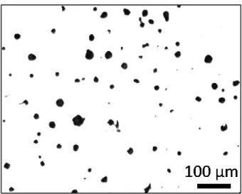
Some typical microstructures of SGI-3 are shown in Figure 2 (thickness: 15 mm), Figure 3 (thickness: 50 mm) and Figure 4 (thickness: 75 mm). As can be seen from these figures, the graphite size tends to become smaller with decreasing plate thickness due to the faster cooling rate, viz., shorter time for graphite growth. The same trend was found for the SGI-2 as well.
Figure 3. Optical micrograph of the SGI-3 specimen; thickness: 50 mm.
Figure 4. Optical micrograph of the SGI-3 specimen; thickness: 75 mm.
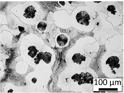
The SGI-3 sample has a fully developed bull’s eye structure (Figure 5) and it was confirmed that all other materials in the current study was fully ferritic, Figures 6 and 7.
Figure 6. Optical micrograph of the SGI-1 specimen; thickness: 50 mm (Fully ferritic).
Figure 7. Optical micrograph of the CGI-2 specimen; thickness: 75 mm (Fully ferritic).
3.2. Coefficient of Thermal Expansion (CTE)
Figures 8–10 show the CTE of sample SGI-2, SGI-3 and CGI-2, respectively.
Figure 8. Coefficient of thermal expansion (CTE) of SGI-3 (15, 50 and 75 mm) as a
As can be seen in Figure 8, the CTE tends to increase with increasing ferrite amounts in the matrix (ferrite amount: SGI-3, 15 mm = 34%, SGI-3, 50 mm and 75 mm = 39%) and the trend agrees with the literature data [9].
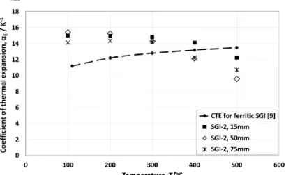
Figure 9. CTE of SGI-2 (15, 50 and 75 mm) as a function of temperature (during heating cycles).
The SGI-2 samples are fully ferritic. In this case, the results can be explained by the graphite amount in the microstructure. As shown in Table 3, the graphite amount in SGI-2, 15, 50 and 75 mm, are 2.12%, 6.78% and 5.57%, respectively, and the CTE is decreasing with increasing graphite (which has much lower CTE than matrix) amounts (Figure 9). The matrices of SGI-2 samples are 100% ferritic. Therefore, there is no influence of the ferrite/pearlite ratio and graphite amount is a dominant factor.
On the other hand, in the case of ferrite/pearlite matrix (SGI-3 in Figure 8), the samples that have higher graphite amounts (SGI-3, 50 mm and 75 mm) show higher CTE. This opposite trend indicates that the ferrite/pearlite ratio plays a more important role than graphite amount.
Figure 10. CTE of CGI-2 (15, 50 and 75 mm), as a function of temperature (during heating cycles).
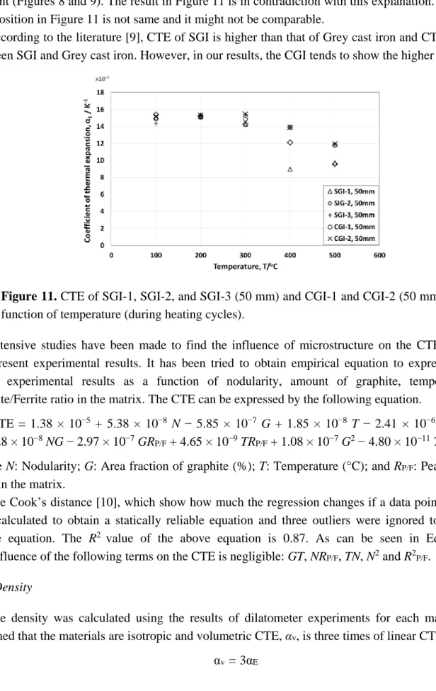
The graphite amount in CGI-2, 15, 50 and 75 mm, are almost the same (about 2%) and it seems there is no relation between nodularity and CTE (Figure 10). The CTE of the SGI and CGI cast irons are summarized in Figure 11.
For the samples that have fully ferritic matrix and higher graphite (which has a much lower CTE than matrix) amounts tend to show the lower CTE.
The SGI-3 (which has lowest ferrite in matrix) shows the higher CTE. In the previous section, it has been concluded that the ferrite/pearlite ratio are playing a more important role than the graphite amount (Figures 8 and 9). The result in Figure 11 is in contradiction with this explanation. The sample composition in Figure 11 is not same and it might not be comparable.
According to the literature [9], CTE of SGI is higher than that of Grey cast iron and CTE of CGI is between SGI and Grey cast iron. However, in our results, the CGI tends to show the higher CTE.
Figure 11. CTE of SGI-1, SGI-2, and SGI-3 (50 mm) and CGI-1 and CGI-2 (50 mm) as a
function of temperature (during heating cycles).
Extensive studies have been made to find the influence of microstructure on the CTEs based on the present experimental results. It has been tried to obtain empirical equation to express the CTE using experimental results as a function of nodularity, amount of graphite, temperature and Pearlite/Ferrite ratio in the matrix. The CTE can be expressed by the following equation.
CTE = 1.38 × 10⁻⁵ + 5.38 × 10⁻⁸ N − 5.85 × 10⁻⁷ G + 1.85 × 10⁻⁸ T − 2.41 × 10⁻⁶ RP/F − 1.28 × 10⁻⁸ NG − 2.97 × 10⁻⁷ GR
P/F + 4.65 × 10⁻⁹ TRP/F + 1.08 × 10⁻⁷ G2 − 4.80 × 10⁻¹¹ T2
(2) where N: Nodularity; G: Area fraction of graphite (%); T: Temperature (°C); and RP/F: Pearlite/Ferrite ratio in the matrix.
The Cook’s distance [10], which show how much the regression changes if a data point is deleted, was calculated to obtain a statically reliable equation and three outliers were ignored to derive the above equation. The R2 value of the above equation is 0.87. As can be seen in Equation (1), the influence of the following terms on the CTE is negligible: GT, NRP/F, TN, N2 and R2P/F.
3.3. Density
The density was calculated using the results of dilatometer experiments for each material. It is assumed that the materials are isotropic and volumetric CTE, αv, is three times of linear CTE, αE.
The density at room temperature was measured by Archimedes’ method and the results are shown in Table 4.
Table 4. Density at room temperature (g∙cm−3).
Thickness SGI-1 SGI-2 SGI-3 CGI-1 CGI-2
15 mm - 7.04 7.11 - 7.06
50 mm 7.02 7.04 7.10 7.04 7.04
75 mm - 7.04 7.10 - 7.05
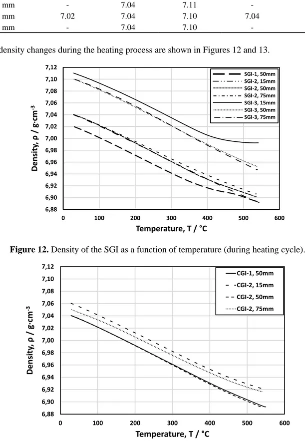
The density changes during the heating process are shown in Figures 12 and 13.
Figure 12. Density of the SGI as a function of temperature (during heating cycle).
Figure 13. Density of the CGI as a function of temperature (during heating cycle).
6,88 6,90 6,92 6,94 6,96 6,98 7,00 7,02 7,04 7,06 7,08 7,10 7,12 0 100 200 300 400 500 600 Density , ρ / g· cm -3 Temperature, T / °C SGI-1, 50mm SGI-2, 15mm SGI-2, 50mm SGI-2, 75mm SGI-3, 15mm SGI-3, 50mm SGI-3, 75mm 6,88 6,90 6,92 6,94 6,96 6,98 7,00 7,02 7,04 7,06 7,08 7,10 7,12 0 100 200 300 400 500 600 Densit y, ρ / g· cm -3 Temperature, T / °C CGI-1, 50mm CGI-2, 15mm CGI-2, 50mm CGI-2, 75mm
3.4. Effect of Thermal Cycling on Thermal Expansion
The dL/L0 values at 55 °C are plotted against the number of cycles and shown in Figures 14 and 15.
Figure 14. Thermal expansion behavior of the SGI-1 (thickness: 30 mm) during thermal
cycling (dL/L0 at 55 °C).
As shown in Figure 14, for the SGI-1, the dL/L0 at 55 °C was decreased from the beginning and became constant. The SGI-1 has a ferritic matrix, as shown in Figure 6. However, the decomposition of retained cementite into graphite and ferrite might occur in the vicinity of the maximum temperature in the measurement (600 °C), since the samples contains relatively high silicon. Usually, the volume is increased by the graphitizing. However, in the present case, the vacancy or pores of already existing graphite phase seem to be filled with the decomposed carbon and the influence of the filling of the pore with carbon is superior to the volume expansion due to the graphitizing. As a result, the total volume seems to become smaller. The volume change seems to occur by the competition of these two effects.
Figure 15. Thermal expansion behavior of the SGI-3 (thickness: 30 mm) during thermal
cycling (dL/L0 at 55 °C). 0,0 0,2 0,4 0,6 0,8 1,0 1,2 0 10 20 30 40 50 dL/ L 0 Cycle x10-3 0,0 0,2 0,4 0,6 0,8 1,0 1,2 0 10 20 30 40 50 dL/ L 0 Cycle x10-3
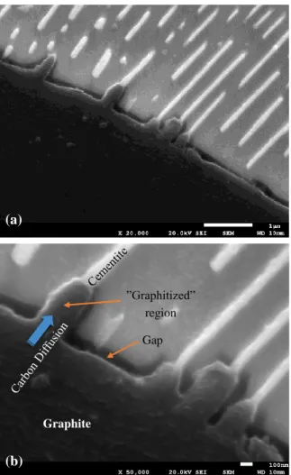
For the SGI-3, the volume was increased in the first cycle. In this case, the increasing of volume due to the graphitizing might be superior to the shrinkage by the filling effect and the total volume seems be increased in the first cycle. In the cycle test, the volume of the SGI-3 is increased in the first cycle. However, in the single cycle experiment, the volume of the SGI-3 is decreased from beginning as SGI-1. It implies that the trend of volume change depends on the amount of pore or vacancy in the graphite phase. In the cycle test, the volume starts to decrease from the second cycle and after the incubation time, that is, the stage where the increasing of the volume due to the local graphitization and the decreasing of the volume due to the filling effect is balanced, the volume is increased again. The volume is increased constantly after 15 cycles. This might be an influence of constant change of phases and microstructure, that is, the phase and microstructure are approaching to the steady state under the present experimental condition and continuous decomposition of cementite. The SEM images of SGI-3 before and after the cycle tests are shown in Figure 16. The SGI-3 has bull’s eye structure as shown in Figure 5. However, some graphite ais surrounded by pearlite as, shown in Figure 16, and the bridges of cementite were observed between the graphite and matrix. These bridges might be acting as a bypass for the carbon diffusion. As can be seen in Figure 16b, it was observed that the cementite bridges on the graphite side is graphitized after the cycle tests. The volume seems to be expanded due to the local graphitization. In addition, the binding between the original graphite phase and matrix might become loose and the gap might become larger due to the graphitizing of the cementite bridge. Figure 17 shows this phenomenon in more details.
Figure 16. SEM images of SGI-3 (a) before and (b) after thermal cycling tests.
(a)
Figure 17. SEM images of SGI-3 showing local graphitization after cycling test, in two
different magnifications: (a) low magnification and (b) high magnification.
For the qualitative justification, more investigation on the relative atomic volume change of Fe3C and graphite is required.
3.5. Uncertainty of Measurements
The experimental results were assessed based on Guide to the expression of Uncertainty in Measurement (GUM) [11,12]. The values of each factor are summarized in the Appendix A.
3.5.1. Uncertainty of αRS
The CTE of reference material is 8.00 × 10⁻⁶ ± 0.1 × 10⁻⁶ K−1 at 300 °C. Hence the uncertainty of the αRS can be described by the following equation.
6 2 8 1 RS 1 0.1 10 (α ) ( ) d 5.8 10 (K ) 2 3 3 m a m a a u x m x a
(4)where m is the standard value and a is the tolerance. 3.5.2. Uncertainty of δαRS
The uncertainty of δαRS can be assessed as follows.
Graphite ”Graphitized” region Gap (b) (a)
u (δαRS) = u (q × ΔT) (5) where q is the slope of αRS against temperature, which is obtained by least-square method. In the present paper, the standard αRS values at 275, 300 and 325 °C were used to obtain the slope. The uncertainty of q depends on the uncertainty of αRS and it can be described as follows.
8 RS 9 2 2 k (α ) 5.8 10 ( ) 1.7 10 (K ) 35 ( ) u u q T T
(6)where T is the average of the three temperatures, viz., 300 °C. Hence the uncertainty of δαRS at 300 °C is
u (δαRS) = 1.7 × 10−9 × 20 = 3.4 × 10⁻⁸ (K−1) (7) 3.5.3. Uncertainty of δT
The uncertainty of the δT can be estimated from the sample deformation during the measurement. The tolerance of the melting point due to the impurity of the sample was assumed ±0.5 °C.
The uncertainty of the reading of values were assumed to be 0.2 °C (standard deviation). The resolution of the temperature measurement is 0.1 °C, viz., tolerance is ±0.05 °C.
The δT will be changed by the sample position and thermal property of the sample and the reproducibility of the measurement is assumed to be 0.5 °C (standard deviation) in the present measurement.
Hence the uncertainty of the δT at melting point can be described as follows:
2 2 2 2 mp 0.5 0.05 (δ ) (0.2) (0.5) 0.61(K) 3 3 u T (8)
The δT at 300 °C can be obtained from the melting points of Tin (Tmp,Sn = 231.9 °C) and Lead (Tmp,Zn = 327.5 °C) by the Linear interpolation.
mp,Sn Zn Sn Sn mp,Zn mp,Sn 300 δT T (δT δT ) δT T T (9)
Furthermore, it may be arranged as follows:
mp,Sn mp,Zn Zn Sn Zn Sn mp,Zn mp,Sn ( ) / 2 1 δ (δ δ ) (δ δ ) 2 T T T T T T T T T T . (10)
Hence, the uncertainty of δT at 300 °C is
2 mp,Sn mp,Zn 2 mp mp,Zn mp,Sn 300 1 2 (δ ) 2 2 ( ) (δ ) 0.47(K) 2 T T u T u T T T (11)
3.5.4. Uncertainty of δT * 2 2 mp,Sn mp,Zn mp,Zn mp,Sn 2 2 (δ *) (δ ) (δ ) 20 (0.21) (0.21) 0.062(K) 327.5 231.9 T u T u T u T T T (12) 3.5.5. Uncertainties of m RS ΔL ( )T and Δ m ( ) X L T The uncertainties of m RS ΔL ( )T and Δ m ( ) X
L T depend on the resolution of the displacement transducer. The resolution of transducer is 1.25 nm and the ΔL was derived from the measurement at two different temperatures, viz., at T ± ΔT/2. Hence the uncertainties of ΔLmRS( )T and ΔL TmX( ) are
2 9 m 10 1.25 10 2 (Δ ( )) 2 5.1 10 (m) 3 u L T (13) 3.5.6. Uncertainties of LRS0 and LX0
The length of the specimens was measured using a micrometer, which has 0.001 mm resolution and ±0.002 mm nominal accuracy.
The deviation of the temperature from 20 °C is assumed ±5 °C.
2 mic 2 mic 20 2 2 2 2 0 mic mic D 0 2 6 2 2 6 3 RS σ 2 ( ) (σ ) ( ) ( ) ( ) α(20 C) 3 3 3 1 10 2 10 2 5 α (20 C) 12 10 3 3 3 R T u L u u R u T L (14)
where σmic is the nominal accuracy of the micrometer and Rmic is the resolution of the micrometer. As can be seen from the above equation, the CTE at 20 °C, α (20 °C), is required. However, the order of CTE of alumina and cast iron are 10−6 and 10−5, respectively. Hence, the third term in the above equation is negligible. Therefore the uncertainties of LRS0 and LX0, u (L0), is
u (L0) ≈ 1.19 × 10⁻⁶ (m) (15)
3.5.7. Combined Standard Uncertainty
The combined standard uncertainty, uc (αx) can be described by the following equation.
2 2 2 c i i (α )x f ( ) u u x x
(16)where αx (=f(xi)) is the CTE of the sample; xi is the factor of each uncertainty.
As an example, a combined standard uncertainty of the measurement result of SGI-3, 50 mm at 300 °C (αx = 1.54 × 10⁻⁵, αxm = 7.82 × 10⁻⁶, ΔLxm = 1.88 × 10⁻⁶) was evaluated and following value was obtained.
uc (αx) = 6.39×10⁻⁸ (1/K) (17)
4. Conclusions
The CTE and density of SGI and CGI materials were measured as a function of temperature in the temperature range of room temperature to 500 °C (600 °C for the cycle tests).
Based on the microstructure characterization, empirical equations for the CTE were derived and it can be described by the following equation:
CTE = 1.38 × 10⁻⁵ + 5.38 × 10⁻⁸ N – 5.85 × 10⁻⁷ G + 1.85 × 10⁻⁸ T − 2.41 × 10⁻⁶ RP/F − 1.28 × 10⁻⁸ NG − 2.97 × 10⁻⁷ GR
P/F + 4.65 × 10⁻⁹ RP/F + 1.08 × 10⁻⁷ G2 − 4.80 × 10⁻¹¹ T2
(2) N: Nodularity; G: Area fraction of graphite (%); T: Temperature (°C); and RP/F: Pearlite/Ferrite ratio in the matrix.
The expansion and shrinkage at a constant temperature in the cycle tests could be explained by the volume change due to the local graphitization.
The uncertainty of the CTE measurement was assessed using the GUM method and it was assessed that the combined standard uncertainty of the CTE is 6.39 × 10⁻⁸ (1/K) under a specific condition.
Acknowledgments
The authors thank the Knowledge Foundation, CompCast project for their financial supports.
Author Contributions
T.M., E.G. and A.G.S. performed the experiments; T.M. analyzed the data; T.M., E.G. and A.E.W.J. wrote the paper; A.E.W.J. supervised the work; L.E. contributed materials.
Appendix A: Analysis of CTE
The measured sample length at temperature T, L TmA( ), which is detected by the displacement transducer can be described by Equation (18).
m
A A
A( ) ( δ ) PR( ) SC( )
L T L T T L T L T (18)
where T is the temperature measured by the thermocouple; LA (T + δTA) is the length of the sample at sample temperature T + δTA; δTA is the temperature difference between the temperature measured by the thermocouple and the temperature of the sample; LPR (T) is the length of the push rod; and LSC (T) is the length of the sample carrier.
The term LA (T + δTA), in the above equation can be expressed by using the CTE as follows.
A 2 A( δ )A A( ) A0α ( )δA A 1 A0δα δ A 2 Δ L T T L T L T T L T T (19)where LA (T) is the length of the sample at sample temperature T; LA0 is the length of the sample at room temperature; αA(T) is the CTE at temperature T; and δαA is the change of the CTE due to the temperature change, ΔT, in the vicinity of temperature T.
From Equations (18) and (19), the LmA at temperature T + ΔT/2 and T − ΔT/2 can be calculated and the measured CTE at temperature T can be described as follows [10].
m m A A m A 0 A A A PR SC A A A 0 Δ / 2 Δ / 2 α ( ) Δ ( ) ( ) δ * δ δ * α ( ) α ( ) δα Δ Δ Δ Δ L T T L T T T T L L T L T T T T T T T T T T L (20)where L0 is the length of the sample; δTA* is the change of δTA corresponding to the change of temperature T (ΔT).
The α ( )mA T was measured for the alumina (reference) and our samples in the present study. From these values, the term PR SC
S0 ( ) ( ) Δ L T L T T L
in the above equation can be cancelled and the CTE of
the sample at temperature T, αX (T), can be described as follows.
m m
RS Δ RS RS δ δ * α ( ) α ( ) α ( ) α ( ) δα δα Δ δ * Δ Δ δ * X X X T T T T T T T T T T T T (21)where αRS (T) is the CTE of the alumina (reference) at temperature T;
m m 0 Δ ( ) α ( ) Δ X X X L T T T L is
the measured CTE of the sample at temperature T.
m m RS RS RS0 Δ ( ) α ( ) Δ L T T T L
is the measured CTE of
the alumina (reference) at temperature T.
In the present analysis, influence of the sensitivity of the transducer, room temperature change and material dependency of the δTA due to the difference of the thermal conductivity and endo/exothermic reactions were ignored for the sake of simplicity.
The values used to calculate the CTE of the sample at temperature T, αX(T), are summarized in
Table 5.
The value of αRS and δαRS was taken from the Netzsch’s standard [13] for the temperature range from 25 °C to 550 °C.
Table 5. Input values for the calculation of CTEs. Parameters Values αRS 7.78 × 10⁻⁶ (1/K) δαRS 100 °C: 3.60 × 10⁻⁸ (1/K) 200 °C: 1.76 × 10⁻⁷ (1/K) 300 °C: 2.00 × 10⁻⁸ (1/K) 400 °C: −2.00 × 10⁻⁸ (1/K) 500 °C: 2.00 × 10⁻⁸ (1/K) δT 1 (K) δT * 0.01 (K) m RS( ) L T
Measured value at each temperature range
m
( )
X
L T
Measured value at each temperature range
LRS0 1.2 × 10⁻² (m)
LX0 1.2 × 10⁻² (m)
δαX 0 (1/K)
ΔT 20 (K)
Appendix B: List of Symbols
AGraphite (IOS form VI): Surface area of graphite with roundness higher than 0.625 (ISO 945 form VI); AGraphite (IOS form IV+V): Surface area of graphite with roundness between 0.525 and 0.625 (ISO 945 form IV and V);
AGraphite (All): Surface area of all graphite; a: tolerance;
CGI: Compacted Graphite Iron;
CTE: Coefficient of thermal expansion; dL: Change in length;
G: Area fraction of graphite (%); L0: Initial length;
LA (T): Length of the sample at temperature T;
m A( )
L T : Measured sample length at temperature T; LPR (T): Length of the push rod at temperature T; LRS0: initial length of reference sample;
LSC (T): Length of the sample carrier at temperature T; LX0: Initial length of sample X;
m: Standard value; N: Nodularity;
q: Slope of αRS against temperature; Rmic: Resolution of the micrometer; RP/F: Pearlite/Ferrite ratio in the matrix; SGI: Spheroidal Graphite Iron;
T: Temperature of the sample; T: Average temperature;
Tk: Selected temperatures to calculate the CTE; t: Thickness of the component;
u(x): Uncertainty of xαA(T): CTE of sample A at temperature T; αE: Coefficient of thermal expansion (CTE);
αRS: CTE of alumina (reference);
αRS (T): CTE of the alumina (reference) at temperature T;
m m RS RS RS0 Δ ( ) α ( ) Δ L T T T L
: Measured CTE of the alumina (reference) at temperature;
αV: Volumetric CTE; αX: CTE of sample x; m m X X X0 Δ ( ) α ( ) Δ L T T T L
: Measured CTE of the sample at temperature T;
ΔL: Change in length;
m RS( )
L T
: Measured ΔL value of reference sample at each temperature range;
m
( )
X
L T
: Measured ΔL value of sample X at each temperature range; ΔT: Change of temperature;
ΔTD: Deviation of the temperature during the L0 measurement;
δαRS: Change of the CTE of the alumina (reference) due to the temperature change, ΔT, in the vicinity of temperature T;
δαX: Change of the CTE of the sample X due to the temperature change, ΔT, in the vicinity of
temperature T;
δT: Temperature difference between the temperature measured by the thermocouple and the temperature of the sample;
δT*: Change of δT corresponding to the change of temperature T(ΔT);
δTA: Temperature difference between the temperature measured by the thermocouple and the temperature of the sample A;
δTA *: Change of δTA corresponding to the change of temperature T(ΔT) for sample A; δTmp: δT at melting point;
ρ: Density;
σmic: Nominal accuracy of the micrometer.
Conflicts of Interest
The authors declare no conflict of interest.
References
1. Dawson, S. Compacted Graphite Iron—A Material Solution for Modern Diesel Engine Cylinder Blocks and Heads. China Foundry 2009, 6, 241–246.
2. Larker, R. In Solution Strengthened Ferritic Ductile Iron Iso 1083/js/500-10 Provides Superior Consistent Properties in Hydraulic Rotators, In Proceedings of Keith Millis Symposium on Ductile Iron, Las Vegas, NV, USA, 2008; Hilton Head: South California, CA, USA, pp. 169–177. 3. Hollinger, I. Compacted Graphite Cast Iron Alloy. Swedish Patent 9802418-5, 1998.
4. Sieurin, H.; Zander, J.; Sandström, R. Modelling Solid Solution Hardening in Stainless Steels. Mater. Sci. Eng. 2006, 415, 66–71.
5. Fras, E.; Kawalec, M.; Lopez, H.F. Solidification Microstructures and Mechanical Properties of High-Vanadium Fe–C–V and Fe–C–V–Si Alloys. Mater. Sci. Eng. 2009, 524, 193–203.
6. Mampaey, F.; Habets, D.; Plessers, J.; Seutens, F. On Line Oxygen Activity Measurements to Determine Optimal Graphite form during Compacted Graphite Iron Production. Int. J. Metalcasting 2010, 4, 25–43.
7. Selin, M.; König, M. Regression Analysis of Thermal Conductivity based on Measurements of Compacted Graphite Irons. Metall. Mater. Trans. 2009, 40, 3235–3244.
8. ISO 16112:2006, Compacted (Vermicular) Graphite Cast Irons—Classification. Available online: http://www.iso.org/iso/catalogue_detail.htm?csnumber=37724 (accessed on 27 May 2015).
9. Davis, J.R. ASM Specialty Handbook—Cast Irons; ASM International: Geauga County, OH, USA, 1996; pp. 430–432.
10. Cook, R.D. Detection of Influential Observations in Linear Regression. Technometrics 1977, 19, 15–18.
11. Yamada, N. Evaluation of Uncertainty in Thermal Expansivity Measurements. Netsu Sokutei
2002, 29, 72–81.
12. ISO/IEC Guide 98–3:2008, Uncertainty of Measurement—part 3: Guide to the Expression of Uncertainty in Measurement. Available online: http://www.iso.org/iso/catalogue_detail.htm? csnumber=50461 (accessed on 27 May 2015).
13. Netzsch-Gerätebau-GmbH Expansion Tables for Dilatometer Standards; Gerätebau GmbH: Selb, Germany, 1995.
© 2015 by the authors; licensee MDPI, Basel, Switzerland. This article is an open access article distributed under the terms and conditions of the Creative Commons Attribution license (http://creativecommons.org/licenses/by/4.0/).