The impact of trade on human development in Sub-Saharan
Africa (SSA)
MASTER THESIS WITHIN: Economics NUMBER OF CREDITS: 30 Credits
PROGRAMME OF STUDY: Urban, Regional and International Economics AUTHOR: Grace Mbabazi
JÖNKÖPING : August-2017
Master Thesis in Economics
Title: The impact of trade on human development in Sub-Saharan Africa (SSA) Author: Grace Mbabazi
Supervisor: Sara Johansson Date: 2017-08-07
Key Words: Trade, Human development, Sub-Saharan Africa, Panel data analysis
Abstract
Controversy concerning the relationship between trade and development has persisted for centuries. The advocates of free trade link it with income growth but its impact on the welfare of an average citizen remains highly unaddressed in the economic literature. This paper attempts to contribute to the limited literature on trade and human development by examining the impact of trade on income, education, and life expectancy in Sub-Saharan Africa (SSA). By employing a generalized method of moments (GMM) approach in a panel data setting comprising 38 countries and 11 years, the empirical results suggest that an increase in trade is positively associated with enhancement in social welfare in SSA.
Acknowledgements
I would like to express my appreciation to my supervisor Sara Johansson, for her constructive guidance during the planning and development of this research.I would also like to extend my thanks to my parents and siblings, for their support andencouragement throughout my studies.
Table of contents
1.Introduction ... 1
1.1 Overview of the growth of human development in Sub-Saharan Africa ... 3
1.1.1 growth of life expectancy in SSA ... 4
1.1.2 The growth in GNI per capita ... 5
1.1.3 Overview of secondary education enrollment in SSA ... 6
2. Previous researches and theoretical frame ... 8
2.1 Trade and economic growth ... 8
2.2 Trade and human development ... 11
3. Econometric Methodology and Data ... 14
3.1 Data ... 14
3.2 Econometric Methodology ... 15
4. Descriptive statistics ... 20
5. Empirical results and analysis ... 22
5.1 The effects of trade on growth in GNI per capita ... 22
5.2 The effects trade on education ... 24
5.3 The effects of trade on life expectancy ... 26
6. Conclusion ... 29
7. References ... 30
8. Appendix ... 34
1
1.Introduction
The issue of what causes economic growth is widely discussed among economists and is mostly described as an extremely complex process, which depends on many variables such as capital accumulation (both physical and human), trade, price fluctuations, political conditions, income distribution, and even more on geographical characteristics. The export and import-led growth hypothesis postulate that export respectively imports expansion are important driver of economic growth as they allow countries with weak domestic purchasing power to build up domestic industries ahead of growth in domestic demand. In this case, trade (through imports and exports) can foster economic development by providing channels for knowledge and technology inflow.
Over the past decade, Africa’s economy has been experiencing a dynamic growth, with an average income growth rate of 5.07 % per year, between 2005 and 2014(World Bank, 2017). This remarkable performance has nurtured an optimistic ‘Africa rising’ expectation and restored international interest in the continent. However, the “Africa rising” narrative partially overshadows the continent’s continued vulnerabilities such as political crises; that are accompanied by public health emergencies and volatile global markets. Despite the impressive economic performance, Africa is still home to millions of people who live in extreme poverty. An undeniable challenge remains: can the continent’s dynamic economic expansion be converted into sustainable human development?
Scholars have addressed the issue of overall African economic development, but the developmental effect on the average African citizen remains unclear and largely unaddressed. Studies that bring out the African economic development are often met with a counterargument that “development” should imply more than rising incomes. Taking this argument as a base and by focusing on trade in particular, this study examines the impact of trade on welfare, measured by the Human Development Index (HDI), in Sub-Saharan Africa. More specifically, the research question is formulated as follows: What impact does trade have on human development in Sub-Saharan Africa (SSA)? Studies ( e.g Asongu, 2012) have attempted to addressed a more or less similar research question. However, the distinctive feature of this study in contrast to other studies is the size of the sample countries, the time period as well as the econometric approach to address the research question.
This research aims to expand the development debate by focusing on the impact of trade on wider social development indicators in Sub-Saharan Africa (SSA). Hence, the variables in
2
focus in this empirical analysis is total trade per capita (exports + imports) which is presumed to have a positive impact on social development. In pursuit of examining the relationship between the two factors, several studies use trade as a share of GDP. However, the logic presented in the study of Davies and Quinlivan (2006) is that, since the focus of the research is on human development; the main concern should be on trade per capita, as it affects the individual citizen. The use of the metric trade per-capita should therefore be more appropriate than the ratio of trade to GDP.
As mentioned earlier, development signifies not just economic growth but also human advancement. Putting in consideration this argument, economic data alone is insufficient to measure the contribution of trade to development. Consequently, this study utilizes the components of the HDI index as indicators of both social and economic development. The HDI index measures a country‘s performance in three human development dimensions: decent standard of living, a long and healthy life as well as knowledge. The individual components of the HDI index in this study therefore include Gross National Income (GNI) Per Capita, life expectancy at birth and Gross enrollment in secondary education.
This research employs Generalized Method of Moments (GMM) estimation approach developed for dynamic panel data models in order to deal with the potential endogeneity bias. Estimations are performed on an unbalanced panel data of 38 countries sub-Saharan countries over the period of 2004 -2014. As it was mentioned earlier, the dependent variables are the mentioned components of HDI and trade per capita is the ultimate and most important independent variable for this research. The estimations also include various control variables such as government expenditure on health and education, gross capital formation as well as labor force accumulation. In addition to this, this study considers observations of the dependent variables as well as trade openness (trade as % GDP) in 2004, to test for the impact of initial conditions. The main results confirm trade per capita has a positive impact on GNI per capita as well as life expectancy in SSA. On the other hand, this research has found insignificant results between trade per capita and enrolment in secondary school in SSA. This research paper is organized as follows: the next paragraph gives an overview of the state of human development in SSA, while section 2,3 and 4 respectively encompass the theoretical framework, explanation of used data and the econometric methodology as well as the descriptive statistics. The last two sections(5 and 6) embodies respectively the empirical results and analysis as well as the conclusion.
3
1.1 Overview of the growth of human development in Sub-Saharan Africa
Historically, Sub-Saharan African countries have faced and are still facing various challenges, including extreme poverty, political instability, and a skewed income distribution. The region is known to be highly corrupted mostly in judicial systems, police departments and governments, as nearly 75 million people in Sub-Saharan Africa are estimated to have paid bribes in 2014 in order to escape punishment; but also to get basic services that they ought to have (Transparency International, 2015). In terms of education, 26% of the global illiterate adults live in Sub-Saharan Africa (UNESCO institute for statistics, 2016). When it gets to transparency, accountability and corruption in public sector rating(CPIA), 30 SSA countries out of the 38 countries that are considered in this study score a combined average of 2,771 out 6, in the period between from 2004 to 20015. Despite the challenges, that hampers development in SSA, during the last decade, the overall region has seen a satisfactory development performance and this has risen an optimistic narrative about the continent. As it is illustrated in the graphs below, since year 2000, the development in Sub-Saharan Africa has seen a considerable growth and has remained stable, even in the face of a hesitant world recovery from the global crisis. One of the main factors that played a significant role in spurring the level of development across the continent is the establishment as well as the implementation of the economic development program NEPAD (New Partnership for Africa's Development ) in 2001; by the African head of states . NEPAD has indeed aimed at implementing a framework for viable development to be shared by all Africans, emphasizing the vitality of partnerships among African nation themselves as well as between them and the international community. This program provided a shared vision to eliminate poverty through reinforcing the pace of regional integration and assistance, especially in the field of security and peace management. These efforts have been backed up by the international community through financial and technical support, as the Heavily Indebted and Poor Countries (HIPC) program was initiated by the International Monetary Fund and the World Bank in 1996. This program provided debt relief as well as low-interest loans to many poor countries, in order to cut down external debt repayments (Sustainable Development Knowledge Platform, 2017).
1SSA CPIA score Source: Author’s calculations using data from the World Bank Development Indicators: CPIA transparency, accountability, and corruption in the public sector rating (1=low to 6=high)
4
On top of the macroeconomic reforms as well as the international supports that has improved the living standard in the region, China –Africa trade has increased tremendously since 2000 (surpassing Africa bilateral trade with the US); and this has contributed to the development of the continent. The high demand from China for the region ’s main exports such as oil, iron, copper, zinc, and other primary products has led to better terms of trade and higher export volumes which has benefited the region (Dollar,2016).
1.1.1 growth of life expectancy in SSA
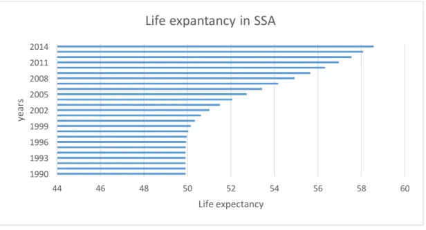
The graph presented below displays the evolution of life expectancy in Sub-Saharan African region, a region that for many years has been characterized by extreme poverty, poor health, wars and political instability. Despite this, the graph below shows a significant growth in life expectancy over the last decade.
Figure 1: The evolution of life expectancy in sub-Saharan Africa from 1990 to 20142.
As it can be observed in the graph above, the average life expectancy in the Sub-Saharan region has gradually grown since 1990. However, the significant growth was experienced from year 2000 to 2014. From 1990 to 2000, the life expectancy grew by less than 1 year during the period 1990-2000, while it grew by approximately 8 years between 2000 and 2014. Countries like Rwanda, Botswana, Malawi, Zimbabwe and Zambia have experience a
tremendous growth since 2000. Malawi, is a one of the success stories as it has managed to
2 Figure 1 is obtained by using aggregates data of the region of Sub-Saharan Africa.
The data is retrieved from World Bank website (World Development Indicators (WDI) database. The statistics that are presented are also retrieved from the World Bank Data base
44 46 48 50 52 54 56 58 60 1990 1993 1996 1999 2002 2005 2008 2011 2014 Life expectancy ye ar s
Life expantancy in SSA
5
improve its life expectancy from only 44, 1 years in 2000 to 62,7 in 2014. For Rwanda, in 1990, the life expectancy was around 34 years and worsened to roughly 29 years in 1994, the year when the ethnical genocide (against Tutsis) was taking place. Six years later, in 2000, the longevity had improved to 48 years and it was trending around 64 years in 2014. Not one sub-Saharan country saw life expectancy fall between 2000 and 2014. Aside from Swaziland (where longevity rose only 0.4 per cent), the smallest improvement was the 2.5 per cent in South Africa.
1.1.2 The growth in GNI per capita
The graph below represents the GNI per capita. GNI per capita is a reasonable first step toward understanding a country’s economic state as it reflects the average income of a country’s citizens.
Figure 2 : The evolution of Gross national income in sub-Saharan Africa from 1990 to 20143
Over the last decade, most Sub-Saharan African countries have recorded economic
advancements at a pace that previously had seemed well out of reach. As it can be seen above, despite the weaker global economic environment, Sub-Saharan Africa have continued to record growth measured in terms of GNI per capita. As it can be seen in figure 2,Regional GNI per capita were actually falling from 1990 to 2000, but after this period the region has seen a strong growth as the GNI per capita rose by more than 3 times, from 505 US$ in 2000 to 1738 US$ in 2014. Even though the overall region has seen growth, there are still countries
3 Figure 2 is obtained by using aggregates data of the region of Sub-Saharan Africa.
The data is retrieved from World Bank website :World Development Indicators (WDI) database. The statistics that are presented are also retrieved from the World Bank Data base
0 200 400 600 800 1000 1200 1400 1600 1800 2000 1990 1991 1992 1993 1994 1995 1996 1997 1998 1999 2000 2001 2002 2003 2004 2005 2006 2007 2008 2009 2010 2011 2012 2013 2014 GN I p er c ap ita years
GNI per capita in SSA
6
that have not performed as well as most of SSA countries. Zimbabwe and Eritrea fell back in terms of improved GNI per capita as their GNI per capita fell on average by - 1, 62% and -2, 61% respectively, in the period after 2000. On the other hand, countries like Equatorial Guinea, Ethiopia, Nigeria and Rwanda have been improving their domestic conditions and consequently have enjoyed solid growth compared to other countries in the region. Their GNI per capita has grown by 8, 3%;7, 06%; 6, 4% and 4,85% respectively after year 2000.
Seychelles and Equatorial Guinea have the largest average GNI per capita in the region, amounting to more than 10 000 US$, while DRC, Liberia and Burundi are amongst the least developed countries in the region with a GNI per capita of less than 300 US$. Hence, there are large differences in income levels even between the African countries. To put things in perspective, Seychelles’ GNI per capita is less than 1/5 (17%) of the one of Sweden’s GNI per capita in 2014 while Burundi’s is 357 times less than the one of Sweden.
1.1.3 Overview of secondary education enrollment in SSA
In today’s increasingly globalized world, countries pursuing growth should strive to build their human capital so that they can be able to compete for jobs and investments. The graph below show the gradual increase of school attainment in the SSA region, a region that includes the large number of countries that have not reached universal schooling goals. As it can be observed, over the period between 2000 and 2014, secondary school enrollment has substantially risen across Sub-Saharan Africa as opposed to the period between 1990 to 2000. 0 10000000 20000000 30000000 40000000 50000000 60000000 1990 1992 1994 1996 1998 2000 2002 2004 2006 2008 2010 2012 2014 num be r o f s tude nt s years
Secondary Education in SSA
7
Figure 3: the evolution of secondary school enrolment in sub-Saharan Africa from 1990 to 20144
As it can be seen in the graph above, the number of students enrolled in secondary school
has increased tremendously since 2000; in comparison to the period between 1990-2014. A cross the region, the average enrolment number in secondary education doubled between 2001 to 2014 (roughly 40 million students) compared with the time- period between 1990 and 2000 where the average was around 20 million students.
Historically, in SSA region, secondary education has largely been reserved for a privileged
few, but many governments have now begun to realize the vitality of investing in a secondary education. In Uganda for example, a government supported public-private partnership is facilitating more adolescents to access a low-cost as well as quality secondary education. For this partnership, nonprofit organizations such as PEAS (Promoting Equality in African Schools) and ARK(Absolute Return for Kids) operate a network of secondary schools, which are financially backed up by the Ugandan government (The Africa- America institute, 2015).
4 Figure 3 is obtained by using aggregates data of the region of Sub-Saharan Africa.
The data is retrieved from World Bank website (World Development Indicators (WDI) database. The statistics that are presented are also retrieved from the World Bank Data base
8
2. Previous researches and theoretical frame
2.1 Trade and economic growth
Theoretical as well as empirical researchers have devoted a considerable amount of energy on determining the drivers of economic growth. One of the most significant theories, Solow (1956), has been the workhorse of growth literature for the past decades. Its main conclusion is that capital and labor force accumulation accelerate the economic growth rate, but that the long run growth depends on an exogenous technology factor. Studies like Barro (1991); Lucas (1988) and Romer (1986) clarify the exogenous ambiguity in Solow (1956) and they specify the economic growth engine. These studies support the hypothesis that productivity depends upon the "stock of knowledge or human capital", a variable that reflects the quantity of people with a college degree (at least) in the local economy. The study of Alesina and Roberto (1996) on the other hand emphasizes that socio-political state of a nation does play a role in
determining growth, as its main conclusion is that social-political instability reduces growth speed.
While some studies amplify the importance of capital, labor and political institutions, other researches lay stress on the vitality of trade in spurring the economic and societal welfare. Explaining the effects of trade on welfare can be extremely complex since the relationship between the two factors are most of the time case specific and endogenous. However, as Davies and Quinlivan (2006) point it out, a general conclusion on the causal correlation between trade openness and decent living standards in a country is through economic growth. As they postulate it, trade openness is considered to be beneficial to economic growth and through growth- poverty reduction. This argument stresses the importance as well as the relevancy of literatures covering the relationship between trade and economic growth. For over two centuries, the theoretical links between economic growth and trade have been discussed; but controversy persists concerning their relationship. The original wave of favorable viewpoints with respect to trade can be traced back to the classical school of economic thought, that began with Smith (1776) who pointed out that trade openness establishes a channel that carries out the surplus products of a country (export). Today, the association between growth and trade is most often linked to the potential favorable
externalities for the economy; arising from participation in world markets, which leads to a more efficient allocation of resources (Heckscher-Ohlin, 1933; Melitz, 2003); economies of scale (Krugman, 1980); productivity gains resulting from increased specialization (Ricardo ,1840); as well as knowledge and technology inflows (Grossman & Helpman, 1991).
9
There is a vast body of empirical work on the relationship between trade and economic development. Dollar and Kraay (2004) stress that open trade regimes lead to faster economic expansion and poverty reduction in less developed countries. This study advocates that countries that have enhanced their exposure to international trade have stimulated their GDP per capita growth, while those that are more reluctant to trade, have not seen a fast growth. Levine and Rentlt (1992) also identify a positive as well as robust association between economic growth and investment share in GDP and between the share of investment and the ratio of international trade to GDP. From cross- country growth studies, the conclusion that appears to be gaining attention in recent years is that most of the countries that achieved growth successfully are also the ones that have embraced the concept of international trade. Martin (2001) and Masson (2001) affirm that these countries have experienced high rates of economic expansion in the context of rapidly growing trade.
The vindication for free trade and the numerous indisputable gains that international
specialization brings to the productivity of nations have been widely discussed and are well documented in the economic literature. However, in the last few decades, there has been a revival of activity in the literature of growth, which has resulted in an extensive stock of models that emphasizes the vitality of trade in spurring economic growth. In pursuit of verifying the hypothesis that open economies advance faster than those that are closed, these models have considered different factors such as the level of openness, tariffs, real exchange rate, terms of trade as well as the export performance in a country ( see Edwards,1998) . Although most studies confirm a positive relation between trade and growth, they also
highlight that trade is one single factor amongst numerous variables that enter into the growth equation. However, various advocates of the Export Led Growth Hypothesis (ELGH) have underlined that trade (through exports) is in fact the main catalyst of growth. The ELGH amplifies that promotion of the export sector is the most effective way to achieve economic growth. A considerable number of studies have revealed various explanations as to why exports are a vital way to obtain growth.
According to Giles and Williams (2000), export catalyze growth in a number of ways. These include supply as well as demand linkages, economies of scale (due to participation in wider international markets), enhanced efficiency, adoption of upgraded technologies (incorporated in foreign-produced capital goods), learning externalities that improves human resources and ameliorated productivity (through specializations and creation of employment). Furthermore, Giles and Williams (2000) argue that embracing trade and having access to world markets
10
may motivate competitive pressure that can boom innovation and facilitate technological improvements as well as knowledge spillovers into the host economy. Krugman and Obstfeld (2006) also affirm that exports may assist exports boom through generating favorable effect on non-exports, enhanced scale economies, ameliorated allocative effectiveness and greater capability to stimulate sustainable comparative advantage.
A considerable number of studies have approached the hypothesis of export led growth through empirical researches. As far back as in 1960s, Emery (1967) presented a hypothesis that a causal association between exports and economic growth do exist, and that this
causation is one of interdependence rather than of unilateral. However, this study affirms that it is mainly an increase in exports that accelerate the speed of overall economic growth rather than vice versa. Other various empirical studies on the link between exports and economic expansion have been conducted on developing economies, utilizing either time- series or cross-section analysis. The first group of studies include Feder (983); Kavoussi (1984) and Michaely (1977) and use cross-country data sets. These studies reveal evidence of ELG hypothesis as they find a positive relationship between export growth and GDP growth. Ekanayake (1999) also test the export led growth hypothesis and his results identify a uni-directional causality that runs from export growth to output expansion. More recent studies such as Allaro (2012) analyzes empirically the export-led growth strategy on Ethiopia's economy. The conclusion of the study supports the existence of unidirectional causality running from export and economic growth. While most of the studies mentioned above support a correlation between exports and economic growth, there are other studies such as Darrat(1987); Rahman & Mustafa (1997) and Sharma & Panagiotidis (2005) that fail to support(for some countries at least) the existence of a significant relationship between the two variables.
Relative to the case for ELG, some theories argue that enhanced level of imports have a considerable role in spurring the overall economic performance. Imports can stimulate the long-run economic growth (especially in developing nations) as they allow the host country to access the needed factors of production, the foreign technology and knowledge (Coe &
Helpman, 1995; Grossman& Helpman, 1991). Awokuse (2008) also postulates that foreign research and development can play a vital role for productivity growth as cutting-edge technologies usually encompass imported intermediate goods such as machines, equipments as well as computers. In this case, foreign imports can be seen as the ultimate sources of technology-intensive factors of production (Lawrence & Weinstein, 1999; Mazumdar, 2001).
11
In addition to this, beyond serving as a carrier of technology, Lawrence and Weinstein (1999) affirm that imports are crucial to productivity expansion since the growth in imports of competing products stimulate innovation; as foreign competition exercise competitive technological pressures on domestic producers.
2.2 Trade and human development
The previous section briefly reviews the literature that is related to the import and export-led strategy, considering in particular the role that trade plays in output growth. However, as this research aims to examine the impact of trade on human development, it is vital to review literatures that pay close attention to the links between trade and the growth of human developmental level. Nevertheless, the basic argument is still resting on the premise that trade’s impact on income growth is the main source of human development in a country. Davies and Quinlivan (2006) point out that the trade effect on output growth is direct, while its influence on non-income measures is indirect and transmitted via income. This study highlights a wider globalist viewpoint that trade affects non-income human development measures both indirectly via income and directly via cross-cultural fertilization as well as augmented range of goods variety. In other words, as Davies and Ouinlivan (2006) advocate it, the standard argument for a positive correlation between human development and trade can be explained in the sense that trade brings about an upgraded living standards in a country, which in turn, yields better health care, better social services, more education etc…
It is true to say that trade stimulates education, considering the fact that conducting business across countries require global awareness, communication and cross-cultural understanding. As it was mentioned earlier, trade generate not only an increase in the quantity of existing goods, but also an extension in the variety of goods consumed. To a developing nation, this implies that the new variety of goods pouring into the country embed medicines, health or education related equipment as well as medical guidance, all of which ameliorate the nutrition, health and longevity of the country’s people. Even if trade had no influence on economic growth, it could be expected that the cross-cultural fertilization that comes along with trade would foster the growth of human development measures, simply by widening people’s perspective as well as exposing the people to new products (Davies & Quinlivan, 2006).
As the increase in trade results in instant income benefits, the indirect effect viewpoint that is presented above can be justified in the sense that the immediate income benefit, in turn,
12
generate long run improvements in literacy and health; as people’s standards of living become greater and the potential returns to education increase. Direct benefits in human development are achieved from the exposure to foreign goods (particularly health related goods) while indirect advantages result from wealth (income) rise in the host country.
Nevertheless, countries in which exposure to trade is controlled, the trade influence on human development might be mitigated. It can be expected that the trade gains are less in countries where consumption of foreign goods is restricted and countries whose trade is conducted by the government instead of private sector (Davies & Quinlivan, 2006).
The study of Fatah, Othman and Abdullah (2012) also estimates the growth rates of China, Indonesia and Malaysia by considering the effects of various HDI components such as longevity, political rights, openness, civil liberties and FDI on income growth. They utilize quantitative models to examine the impact of explanatory variables on economic growth. The conclusion of this study is that openness and HDI have statistically significant and positive effect on economic growth. Eusufzai (1996) poses the question “Can greater growth rates lead to higher development in countries that are open?” He analyzes the relationship between human development and openness. For different types of country group, the Pearson correlation coefficients are calculated between different components of HDI and Dollar’s Openness Index. In conclusion, this study finds a positive and high relationship between openness and HDI. Villanueva (1994) employs neoclassic approaches in his study and concludes that government policies influence the endogenous steady state growth rate of output. In addition to this, he postulates that a large part of the growth patterns across countries is associated to the level of economic openness, the extent of human development and the quality of fiscal policy in a country.
Another study that examines the effect of openness on human development is conducted by Nourzad and Powell (2003). This study conducts a panel data analysis for forty-seven developing countries and utilizes various openness descriptions such as total trade volume over GDP, Dollar’s openness index and black market premium. Two main regression models are employed. In the first regression, they evaluate the impact of openness through the variables such as accessibility of clean water sources, infant mortality rates, government expenditure on education, real GDP and urban population growth rates on HDI. In the second, they analyze the impact of openness, HDI and the other variables on real GDP. In conclusion, their result reveal that there is a positive relationship between openness (total trade over GDP) and real GDP as well as the Human development index.
13
Reuveny and Li (2003) take GINI coefficient as an indicator of income equality and examines the impact that openness and democracy have on income inequality. The study uses pooled time series analysis for 69 countries in order to control their hypothesis. In addition to this, one decade lagged Gini coefficient, education spending and GDP per capita are taken as control variables. In conclusion, the study finds statistically significant coefficient in openness for both less developed as well as developed countries. In the study that is conducted by Asongu (2013), two stage least squares instrumental variable methodology is employed to test the trade and financial openness’ effects on 52 African countries’ human development
measure. The study considers period ranged between 1996 and 2010 and its conclusion is that trade openness positively influence human development, but that financial openness has the opposite impact on human development in the African countries. In this study, the “life expectancy” component of the HDI weighs most in the positive impact of trade globalization on human development.
Other recent studies such as Razmi and Yavari (2012) as well as Kabadayı (2013) evaluate whether being open market oriented benefits societies as a whole. The study of Kabadayi (2013) utilizes a panel data analysis to estimate the effects of trade openness on measures of living standards of medium high-income level countries. In this study, HDI is taken into account as a life standards indicator. In conclusion, this study finds a positive effect of openness on living standards. Razmi and Yavari (2012)’s study examines the effect of trade openness on human development in some oil-rich developing countries. Their results reveal that trade openness significantly affect human development. Basu and Bhattarai (2012) also find a significant positive relationship between the trade share and educational spending to GDP, amplifying that countries that are more open on the trade front also spend more on education.
14
3. Econometric Methodology and Data
3.1 Data
Estimating the impact of trade on development yields three components of the dependent variable: economic growth (proxied by GNI per capita) and human development in terms of education and life expectancy. Annual data between 2004 and 2014, for an unbalanced panel of 38 SSA countries is utilized. The countries are selected based on data availability and all data is extracted from the World Bank website (World Development Indicators WDI)
database. Appendix A and B provides the full list of countries in the sample and the extended definition of variables used in this study.
The dependent variables are the followings:
1. GNI per capita: is the natural logarithm of the gross national income and is based on purchasing power parity, expressed in constant 2011 international $.
2. Enrolment in secondary school: is the natural logarithm of the total number of students, enrolled at public and private secondary education institutions, regardless of their age.
3. Life expectancy at birth (total years):is the natural logarithm of the average time an individual is expected to live, based on the mortality rates at the year of birth. The independent variables that are used in the analysis are measured as follows:
1. Trade per capita: is natural logarithm of the sum of exports and imports of goods and services (expressed in current US dollars); divided by the total population.
2. Trade openness at the beginning of the period: is the natural logarithm of a variable that is proxied by the trade as a percentage of GDP in 2004(which is the beginning of the period).
3. Initial value of GNI per capita: is the natural logarithm of the level of GNI per capita in 2004
4. Initial level of secondary school enrollment: Is the natural logarithm of the total number of students enrolled at public and private secondary education institutions, in the beginning of the period (year 2004).
5. Initial level of life expectancy: is the natural logarithm of the level of life expectancy in 2004.
6. Gross capital formation: is the natural logarithm of an investment level proxy, and is formerly known as gross domestic investment. This measure consists of outlays on
15
additions to the fixed assets of the economy plus net changes in the level of inventories. It is expressed in current US dollars
7. The labor force: is the natural logarithm of a variable that comprises people who are at least 15 years; and who supply labor for the production of goods and services during a specified period. This measure encompasses people who are currently employed and people who are unemployed but seeking work as well as first-time job seekers.
8. The government expenditure on health and education: is the natural logarithm of a variable that is computed using the government expenditure on education, total (as % of GDP) and Health expenditure, total (% of GDP). These ratios are multiplied with GDP (in current US$) and are summed up afterwards.
3.2 Econometric Methodology
As it is mentioned earlier, the empirical estimation is run on an unbalanced panel of 38 countries for the period 2004 -2014, where the dependent variables are the three HDI components (GNI per capita, enrolment in secondary school, and life expectancy). The explanatory variables are trade per capita, gross capital formation per capita, total labor force and government expenditure on health and education per capita. In addition to this, the initial level of the dependent variables are included as regressors in their respective estimations while the initial level of trade openness (trade as % of GDP) is included in all estimations. Some of the panels have been found to contain unit root unit root (by using IM- Pesaran-Shin unit root test) so all variables are transformed through first differencing in order to avoid the econometric bias that is caused by non- stationary.
Since the independent variables are likely to be jointly endogenous while the country-specific effects are unobservable and therefore excluded in the estimation, estimating this model by within group estimations or ordinary Least Squares (OLS) would potentially lead to biased results. Thus, Arellano and Bond, 1991 or the System-GMM (Arellano and Bover, 1995; Blundell and Bond, 1998) estimator developed for dynamic panel data models are more appropriate. The ultimate advantage of these estimation methods is that they solve the endogeneity problem, a problem that arises when there is a bidirectional causality between variables. Both these estimation techniques are designed for panel analysis that encompasses some of the following assumptions:
• A dynamic process where the current realizations of the controlled variable are affected by the past ones.
16
•The existence of arbitrarily distributed fixed individual effects.
• Endogenous regressors that are correlated with past and possibly current state of the error • Uncorrelated random errors across individuals.
• A large number of individuals (N) and a small number of time periods. (The panel is “small T, large N”)
Among the GMM estimators, one may choose the first-differenced approach (Arellano and Bond, 1991), which considers lagged levels of explanatory variables instruments in the regression equations in first differences. Taking first-differences erase country-specific fixed-effects, and thereby eliminating the potential bias that may arise due to the omission of time invariant country specific factors that may influence the growth process. Nevertheless, since the time series that are considered in this study might be persistent, the first-differenced GMM estimator might not be effective under these conditions as lagged levels of explanatory
variables are likely to be weak instruments, and this may lead to biased estimates. Consequently, Arellano and Bover (1995), Blundell, and Bond (1998) also known as the System-GMM approach is employed in this research. The substantial advantage of the Arellano–Bover/Blundell–Bond estimator is that it enhances Arellano–Bond (1991) by making an additional assumption that the specific fixed effects are uncorrelated with first differences of instrument variables. In addition to this, this approach does not crave any external instrument to solve the endogeneity problem. This can dramatically enhance efficiency of a model as it allows for the introduction of more instruments.
The general equation of the system GMM estimation is expressed as follows: 1 𝑌$% = 𝛼 + 𝜃𝑌$%*++ 𝛽𝑋$%+ 𝜀$%
In equation (1) 𝑌$% is the dependent variable and Y$%*+ is its lagged value. X$% Is a matrix of
the explanatory variables and 𝜀$% is the error term.
Equation (1) can also be rewritten as:
2 𝛥𝑌$% = (∝ −1)𝑌$%*++ 𝛽𝑋$%+ 𝜀$% And 𝜀$% = 𝜑$ + 𝛿$%
In this particular study, 𝛥𝑌$% represents the change in HDI components of country i (out of N
countries) in year t (out of T years).
𝑋$%: As it was mentioned earlier, 𝑋$% is the vector of regressors and the initial values of 𝑌$% as well as the initial trade opennessare included as explanatory variables and are in matrix X.
17
𝜀$%: is the error term and embodies two components: the fixed effects 𝜑$ ,that take into account time invariant country-specific features( such as geography); and the idiosyncratic shocks, 𝛿$%, that accounts for time-specific effects such as common productivity adjustments
or the global impact of US dollar appreciation.
By extending equation (1), the three equations that are estimated in this study can be expressed as follows:
3 𝑙𝑛 𝐺𝑁𝐼$% = α + δ ln GNI$%*+ + ω ln GNIH + φ ln OpenH + β ln Trade$% +
σln Gkf$% + τ ln govH&E$% + Ϭ ln LF$% + ε$%
4 𝑙𝑛 𝑒𝑑𝑢𝑐$% = α + δ ln educ$%*+ + ω ln educH + φ ln OpenH + βln Trade$%
+ σ ln Gkf$% + τ ln govH&E$% + Ϭ ln LF$% + ε$%
5 𝑙𝑛 𝑙𝑖𝑓𝑒$% = 𝛼 + 𝛿 𝑙𝑛 𝑙𝑖𝑓𝑒$%*+ + 𝜔 𝑙𝑛 𝑙𝑖𝑓𝑒H + 𝜑 𝑙𝑛 𝑂𝑝𝑒𝑛H + 𝛽𝑙𝑛 𝑇𝑟𝑎𝑑𝑒$%
+ 𝜎 𝑙𝑛 𝐺𝑘𝑓$% + 𝜏 𝑙𝑛 𝑔𝑜𝑣𝐻&𝐸$% + Ϭ 𝑙𝑛 𝐿𝐹$% + 𝜀$%
The dependent variables are in natural logarithm and their abbreviations are as follows:
GNIit: the growth of gross national income per capita of country i between period t and period
t-1.
Educit: the growth of gross enrolment in secondary education of country i between period t
and period t-1.
Lifeit: the growth of life expectancy of country i between period t and period t-1.
Explanatory variables are also in natural logarithm and their abbreviations are as follows:
(GNI)0= Initial level of GNI in 2004 in country i
(Open)0= Initial level of trade openness of country i in 2004 Educ0= initial level of secondary enrolment of country i in 2004 Life0= initial level of life expectancy of country i in 2004 Tradeit: the growth of trade per capita
Gkfit: the growth of gross capital formation per capita
govH&Eit: the growth of government expenditure on health and education per capita LFit: the growth of total labor force
18
As it was mentioned earlier, the effects of trade on human development generate two components, which are economic growth and social development (through education and health). In this study, the natural logarithm of GNI per capita serves as indicator for the income growth as well as purchasing power, and sheds light on economic state with respect to a country‘s population. The gross enrolment in secondary education on the other hand reflects the potential future human capital of the countries; while life expectancy is an indicator of a population wellbeing, that result from improved nutrition, upgraded hygiene, access to clean water, effective immunization, birth control and various medical
interventions.
The independent variables (gross capital formation per capita and labor force) are included in the estimation as determinants of growth, basing on Solow (1956) theory. To account the technological progress that Solow (1956) advocates, proxies for trade and government expenditure in the empirical are utilized as the potential sources of technological changes. Furthermore, to test the impact of initial conditions of the countries, the initial level of the dependent variables as well as the initial trade openness for year 2004 are included as regressors. These variables allow us to test the applicability of the convergence theory (also known as the catch up effect) in the SSA countries. This theory postulates that poorer economies tend to grow at a faster pace than richer economies, which eventually leads to convergence in income levels. The intuition behind the convergence theory is that the marginal productivity of capital is higher in countries with small capital stocks. Thus,
developing countries have the potential to grow faster than developed countries. Furthermore, poorer countries have the opportunity to replicate the institutions, production methods and technologies of developed countries, which also makes them grow faster. The variable of trade openness is also included in the estimation and is almost as important as the trade per capita. This variable allows to further understanding the extent to which the SSA governments are following through on commitments to create open economies; and their attempt to shape trade policies that contribute to economic growth. In this case, the trade openness variable also serves as a proxy of how the unique characteristics of the countries (e.g trade policies, geographic location etc..) affect their trading as well as their overall development.
In order to test for the reliability of the estimated results, the Arellano – Bond test for
autocorrelation is used to tests for serial correlation in the first-differenced errors. In this test , rejecting the null hypothesis of no serial correlation at order one in the first-differenced errors does not imply that the model is specified incorrectly; because the first difference of
19
independent and identically distributed idiosyncratic errors are usually correlated. On the other hand rejecting the null hypothesis at higher orders implies that the moment conditions are not valid specification tests. In this case, the considered test is performed on the first differenced error term at the second order and the null hypothesis is that the latter is second-order uncorrelated.
Although the GMM estimator handles a large number of econometric problems (e.g
endogeneity, heteroscedasticity etc..) it is important to remember that this methodology has its own short comings. The main drawback of the GMM estimator is the fact that it assumes error cross section independency and this assumption is usually made for identification purpose rather than descriptive accuracy. The GMM estimator conditions a sufficient number of explanatory variables and treats what is left over as a purely idiosyncratic disturbance that is uncorrelated across individuals. In practice however, this approach is likely to be
inadequate to remove all correlated behavior in the errors and this may lead to inaccurate inferences as well as inconsistent estimations. In this particular study, the interdependency across the SSA countries may arise for various unavoidable reasons in practice, such as the presence of spatial correlations specified on the basis of social and economic partnerships (or relative location); as well as due to the existence of unobserved components that give rise to a common factor that may affect most of the countries in the region. Another deficiency of this estimation technique (GMM estimator) is that it is not suitable for panels with long time series. This implies that the true effect of the explanatory variables on the controlled variable may be underestimated or even unclear (by using GMM); as some explanatory variables may not necessary give an immediate, measurable result (the full effect may be lagged).
20
4. Descriptive statistics
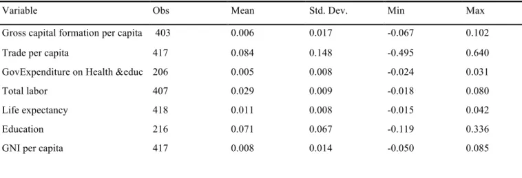
This section presents some descriptive statistics of the variables that are considered in this study; as well as the correlation matrices of the variables in levels and in their growth rates. As it can be noted by the number of observations per variable (in table 1), the panel is highly unbalanced. Furthermore, as it is expected, there are variables that are highly correlated with each other with both in levels and in growth rates (as it is presented in table 2and 3).
Table 1: Descriptive statistics of the variables’ growth rates
Variable Obs Mean Std. Dev. Min Max
Gross capital formation per capita 403 0.006 0.017 -0.067 0.102
Trade per capita 417 0.084 0.148 -0.495 0.640
GovExpenditure on Health &educ 206 0.005 0.008 -0.024 0.031
Total labor 407 0.029 0.009 -0.018 0.080
Life expectancy 418 0.011 0.008 -0.015 0.042
Education 216 0.071 0.067 -0.119 0.336
GNI per capita 417 0.008 0.014 -0.050 0.085
Table 1 embodies calculations of the mean, standard deviation, the minimum as well as the maximum values of the variables’ growth rates. As it reflected by the values of the minimum mean growth rate, some countries in Sub Saharan-Africa region have experienced negative growth rates in different variables. As it is displayed in the table, there is a huge difference between the growth rates of countries that has grown faster (as illustrated by the maximum values of the growth) and the minimum values in the region.
Table 2 Correlation matrix of the variables in levels5
Trade per capita G.exp h&Ed pc Labor force total Life expectancy Capital formation Enrol- in sec Educ GNI per capita Trade per capita 1.000
Gov.exp one health&Educ 0.929 1.000
Labor force -0.458 -0.587 1.000
Life expectancy 0.357 0.394 -0.380 1.000
Gross capital formation 0.916 0.937 -0.682 0.505 1.000 Enrolment in secondary
educ -0.131 -0.276 0.899 -0.247 -0.407 1.000
GNI per capita 0.984 0.882 -0.409 0.335 0.882 0.0756 1.000
5 The correlation matrix presented in table 2 and 3 are the results of the Pearson correlation test, which is a common measure of the degree of the relationship between linearly related variables.
21
As it can be seen in table 2 (where the variables are in levels), the per capita trade, the government expenditure on health and education per capita, as well as the gross capital formation per capita are highly as well as positively correlated with the gross national income per capita. The correlation coefficient value of the enrollment in secondary education is also positive but close to 0, indicating that the relationship between the GNI per capita and
variable is weak for this particular time period that is considered in this study. The coefficient of the labor force variable on the other hand exhibits a negative sign, which implies that this variable negatively affects the income in SSA.
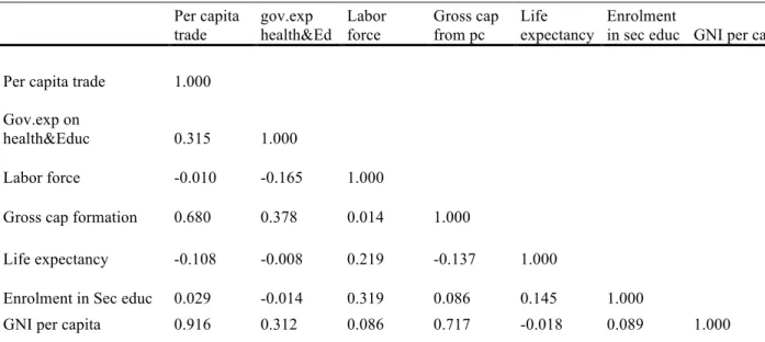
Table 3: Correlation matrix of the variables’ growth rates
Per capita trade gov.exp health&Ed Labor force Gross cap from pc Life expectancy Enrolment
in sec educ GNI per capita Per capita trade 1.000
Gov.exp on
health&Educ 0.315 1.000
Labor force -0.010 -0.165 1.000
Gross cap formation 0.680 0.378 0.014 1.000
Life expectancy -0.108 -0.008 0.219 -0.137 1.000
Enrolment in Sec educ 0.029 -0.014 0.319 0.086 0.145 1.000
GNI per capita 0.916 0.312 0.086 0.717 -0.018 0.089 1.000
Table 3 displays the strengths of association between the variables growth rates. As it can be seen, the growth in trade per capita as well as gross capital formation per capita is still very highly and positively correlated with the growth in income(even though the correlation between the variables is stronger in the their levels). On the other hand, the strength of correlation between income growth and government expenditure on health and education is not as strong as the one in levels as the coefficient is only 0.312, which is quite far from one.
22
5. Empirical results and analysis
This section presents the regression as well as the Arellano-Bond test results, and discusses the effects of trade on the different components of human development. The analysis is sub dived into three sections where section 1, 2 and 3 discuss the effect of trade on GNI, education and life expectancy respectively. Each section encompasses five model specifications, where independent variables are step wisely excluded from the estimations. This allows to test whether the model used in the analysis is correctly specified and that is there is no specification bias or specification error.
5.1 The effects of trade on growth in GNI per capita
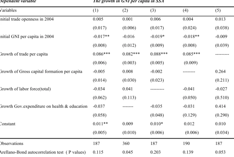
Table 1 presents the estimation results of the first section in the analysis. In this section, the dependent variable is GNI per capita while the regressors include: growth in trade per capita, the time invariant variables (Initial GNI per capita and trade openness), as well as the control variables which are: the growth of total labor force, gross capital formation and the
government expenditure on health and education. As it was mentioned, it is a five model specifications, where the first specification include all independent variables. As it can be seen, specification 1 shows that per capita trade (the variable of the main interest for this research) is significant at 1% significance level. The results indicate that a 1% increase in the growth rate of trade per capita leads to increases by 0,086% in GNI per capita growth. In addition to this, specification 1 shows that the initial value of GNI per capita is significant at 5%. At this significance level, the results show that the growth rate of GNI per capita
decreases by 0,017% as response to a 1% increase in the initial level of GNI. However, all other variables are insignificant in this specification and the Arrelano –Bond test for
autocorrelation fails to reject the null hypothesis of no serial autocorrelation in the errors. The failure to reject the null implies that the estimations are reliable. In specification 2, the control variable of government expenditure on health and education is excluded and all other
variables are insignificant except from trade per capita. The coefficient of trade per capita behaves in the same fashion as in specification 1 (significant at 1%) and increase GNI per capita growth by 0,082%. However, as it can be seen, the P-value of the Arellano-Bond test is less than 5% and this implies that in this particular specification, there is serial autocorrelation in the errors at the second order. In specification 3 and 4, the growth rate of total labor force and gross capital formation per capita are excluded respectively. Here again, in the two specifications, the coefficient of the growth rate of trade per capita is significant at 1%, and the GNI growth is accelerated by 0,088% and 0,085% respectively as response to a unit
23
increase in the independent variable. In addition to this, in specification 3 and 4 , the Initial GNI is significant at 10% and 5% respectively as the growth of GNI per capita decelerates by 0,0185% and 0,0177% respectively, due to an increase in the initial level. In the two specifications, the P values of Arellano-Bond test for zero autocorrelation are greater than 5% and this signifies that there is no autocorrelation in the first differenced errors( at the second order). In Specification 5, when the trade per capita variable is excluded, all variables become insignificant and the autocorrelation test rejects the null hypothesis. In all specifications, the effects of the initial trade openness as well as the growth in capital formation per capita, labor force and government spending on health and education per capita on GNI per capita are unclear.
Table 4: Regression results: The effects of trade on growth in GNI per capita
Dependent variable The growth in GNI per capita in SSA
Variables (1) (2) (3) (4) (5)
Initial trade openness in 2004 0.005 0.001 0.006 0.004 0.013 (0.017) (0.006) (0.017) (0.024) (0.038) Initial GNI per capita in 2004 -0.017** -0.016 -0.019* -0.018** -0.009
(0.008) (0.012) (0.009) (0.008) (0.039) Growth of trade per capita 0.086*** 0.082*** 0.088*** 0.085*** ---
(0.006) (0.003) (0.005) (0.009)
Growth of Gross capital formation per capita -0.005 0.008 -0.002 --- 0.264 (0.014) (0.030) (0.023) (0.211) Growth of labor force(total) -0.034 0.041 --- -0.041 -0.027
(0.062) (0.113) (0.050) (0.510) Growth Gov.expenditure on health & education -0.037 --- -0.035 -0.031 0.414
(0.058) (0.048) (0.129) (0.290)
Constant 0.011** 0.009 0.010* 0.012 0.010
(0.005) (0.010) (0.006) (0.006) (0.034)
Observations 187 360 187 190 187
Arellano-Bond autocorrelation test ( P values) 0.115 0.045 0.203 0.139 0.053
Robust standard errors in parenthesis: * p<0.1; ** p<0.05; *** p<0.001
As it was mentioned earlier, Sub-Saharan African countries have and are still facing various growth challenges resulting from their stagnation in development, political instability and inefficient income distributions. Despite all the serious drawbacks that dismantle the growth process, the growth in trade seem to increase income of the average SSA citizen. The
24
significant positive effect of trade per capita on growth in income jibes with findings of several previous studies (eg. Giles and Williams 2000; Krugman and Obstfeld, 2006). Krugman and Obstfeld (2006) discuss how trade affect production capabilities in a country by giving country the ability to import high quality inputs (mainly capital goods), for
domestic production and exports. Giles and Williams (2000) also affirm that engaging in trade can deflect production in favor of the most growth-contributing industries, which in their turn enhances the capability of human resources, through an upgrade in the overall skill level of the host economy. For the underdeveloped countries in particular (such as SSA), the results are in line with (Awokuse,2008; Coe &Helpman,1995; Grossman & Helpman,1991;
Lawrence & Weinstein, 1999; Mazumdar, 2001); who as mentioned earlier postulate that trade through imports provide much needed factors of production; and that the transfer of technology from developed to developing countries (via imports) could serve as an important source of economic growth. In this study, the coefficient of the initial GNI per capita is significant in 3 specifications. This finding supports theory of convergence as it affirms that poor economies in SSA have grown faster compared to economies who had relatively higher income in 2004. As it was explained earlier, the logic behind this statement is that due to diminishing returns, countries with little physical capital and human capital have higher marginal productivity of capital and human capital, which leads to faster growth. In addition to this, the poorer nations can grow much faster because of higher growth possibilities like access to technological know-how from the more developed nations.
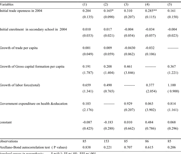
5.2 The effects trade on education
Sometimes openness to trade may have negative impact on school enrolment especially in underdeveloped countries, as foreign traders (or investors) might be attracted to the countries due to their lax labor standards, low wages and an abundant supply of unskilled labor
(including child laborers). However, in this study, the optimistic view on trade openness is supported since the results indicate that the initial trade openness in the SSA has a positive impact on the growth of enrolment in secondary school in SSA. In this section of the analysis, the controlled variables is the gross enrolment in secondary education, while the independent variables include - the initial trade openness and enrolment in secondary school, as well as the growth of trade per capita, total labor force, gross capital formation and the government expenditure on health and education. The specification in this section are designed in the same fashion as the previous section. specification 1 includes all variables while specification 2,3, 4 and 5 excludes respectively the growth in government expenditure on health and education,
25
total labor force, gross capital formation and trade per capita. As it is displayed in the table 3, trade openness is significant at 5% in specification 4 and at 10% in specification 2. Holding everything else constant, a 1% increase in the initial level of trade openness accelerates the growth in enrolment in secondary school by approximately 0,165% and 0,285% respectively. In addition to this, in all specifications, the P values of Arellano-Bond test for zero
autocorrelation are greater than 5% which imply that there is no autocorrelation in the first differenced errors at the second order.
Table 5: Regression results: The effects of trade on growth Education
Dependent variable The growth in Secondary school enrollment in SSA
Variables (1) (2) (3) (4) (5)
Initial trade openness in 2004 0.204 0.165* 0.310 0.285** 0.161 (0.135) (0.090) (0.207) (0.115) (0.158) Initial enrolment in secondary school in 2004 0.010 0.017 -0.004 -0.034 -0.004
(0.033) (0.021) (0.054) (0.057) (0.023) Growth of trade per capita 0.001 0.009 -0.0430 -0.032 ---
(0.049) (0.059) (0.062) (0.106)
Growth of Gross capital formation per capita 0.191 0.208 0.461 --- 0.367 (1.787) (1.404) (3.846) (1.221) Growth of labor force(total) 0.659 0.490 --- 0.377 1.100
(1.341) (0.765) (2.054) ( 0.900) Government expenditure on health &education 0.103 --- 0.929 0.063 0.814
(2.176) (0.207) (3.902) (1.161)
constant -0.087 -0.183 0.010 0.484 0.068
(0.425) (0.288) (0.662) (0.786) (0.296)
observations 85 153 85 86 85
Arellano-Bond autocorrelation test ( P values) 0.838 0.221 0.707 0.615 0.206 Standard errors in parenthesis: * p<0,1; ** p<.05; *** p<.001
The results seem to jibe with Basu and Bhattarai ( 2012) findings as they also find that trade openness leads to higher education (and vice versa) and that a shortage of imported physical
26
capital makes it necessary for the economy to open up to international trade. Davies and Quinlivan (2006) also affirm that trade stimulates education since conducting business across countries require global awareness, communication and cross-cultural understanding.
Theoretically, the effects of the rest of the variables are expected to be positive, especially the government expenditure on health and education. However, it is important to remember that the effects of many variables on education do not necessarily give an immediate, measurable result as the full effect might be lagged. In this case, as this study considers a very short time period (2004 to 2014), the effects of the independent variables on the school enrolment might be underestimated, as the full impact on education may not be observable over this period.
5.3 The effects of trade on life expectancy
As it can be seen from the table 4, in specification 1, where all variables are included, the growth in trade per capita, seem to have a positive impact on the growth of the life expectancy while the growth of total labor force has a negative impact on the longevity in SSA. As it can be seen in this specification, the null hypothesis of the Arellano –Bond autocorrelation test is not rejected and a 1 % increase in the growth rate of trade per capita result in an increase of 0,0011% in the growth of life expectancy. On the other hand, a 1% increase in the growth rate of labor force decreases the life expectancy growth by 0,056%. In specification 2, where the variable of government expenditure on health and education is left out, the coefficient of initial level of life expectancy and trade per capita are significant at 1% and 10% respectively; while gross capital formation as well as total labor force are significant at 5% significance level. The result in specification 2 imply that a 1% increase in the growth rate of trade per capita as well as gross capital formation results in an additional life expectancy growth of 0.00082% and 0 .007% respectively. On the other hand, the initial life expectancy as well as the growth of labor force decelerate the life expectancy growth by 0.017% and 0,035% respectively. However, as it can be seen, the null hypothesis of the Arellano–Bond
autocorrelation test is rejected in this specification. While the initial openness to trade variable is insignificant in all specification, the coefficient of initial life expectancy variable are
significant (and negative) in all specifications except specification 1 where all variables are included. The ones of labor force are negative and significant in two specification, which are 2 and 4(where the gross capital formation is excluded from the estimation). The capital formation as well as the trade per capita on the other hand are significant in only specification 1 and 2.
27
Table 6: Regression results: The effects of trade on growth in life expectancy Dependent variable : the growth in Life expectancy
Variables (1) (2) (3) (4) (5)
Initial trade openness in 2004 0.003 -0.001 0.001 0.001 0.002 (0.003) (0.003) (0.003) (0.006) (0.005)
Initial life expectancy in 2004 -0,004 -0.017*** -0.012** -0.009** -0.013*** (0.004) (0.003) (0.005) (0.004) (0.003)
Growth of trade per capita 0.001** 0.001* 0.001 0.001 --- (0.001) (0.005) (0.001) (0.002)
Growth of Gross capital formation per capita -0.004 0.007** -0.001 --- -0.003 (0.007) (0.004) (0.010) (0.275)
Growth of labor force(total) -0.056*** -0.036** --- -0.066** -0.054 (0.010) (0.014) (0.027) (0.388)
Government expenditure on health &education -0.023 --- -0.017 -0.019 -0.010 (0.021) (0.011) (0.028) (0.038) constant 0.021 0.068*** 0.049** 0.040*** 0.014**
(0.017) (0.013) (0.019) (0.015) (0.054)
observation) 187 360 187 190 187
Arellano-Bond autocorrelation test ( P values) 0.193 0.017 0.1436 0.188 0.155 Robust standard errors in parenthesis: * p<0,1; ** p<.05; *** p<.001
The positive significance of trade per capita is in line with previous researches, such as Davies and Quinlivan, (2006), who predict a positive direct or indirect impact of trade on longevity. This study associates human development and per-capita trade by advocating that trade results in some instant income benefits, which in turn, generate long run improvements in literacy and health. The study also amplifies the direct benefits of trade on human
development (especially in developing countries) which are achieved from the exposure to foreign goods (particularly equipment related to health and education). In addition to this, various theories argue that trade promotes diffusion of knowledge as well as technology, which contributes to development (see: Giles &Williams, 2000; Krugman &Obstfeld, 2006;
28
Davies & Quinlivan, 2006; Grossman & Helpman, 1991). Considering these arguments, it is plausible that the adapted technologies contribute to disease surveillance, treatment
prevention, and more rapid scientific discoveries especially in underdeveloped countries. Furthermore, in underdeveloped countries, through diffusion of knowledge, trade might facilitate the establishment of virtual communities of support, global advocacy, and action networks to health improvements.
In this study, the coefficient of the initial life expectancy is also significant and this confirm a catch up effect as less healthy countries in SSA seem to have improved more in terms of longevity compared to nations that had relatively higher life expectancy in 2004. As for the other variables (capital accumulation per capita, labor force), their real impact on the SSA economy is supposed to be positive, but as it can be seen in table 3, labor force exhibits an unexpected negative sign and is significant. Theoretically the labor force as well as capital accumulation variables are supposed to have a positive impact on output as the two variables are amongst production factors ( Solow ,1956). However, the labor force that is considered in this study only refers to people who are at least 15 years old, who supply labor for the production in SSA ( see appendix B). As mentioned earlier, the illiteracy level is high in SSA and the accumulation of the variable in the SSA countries, does not necessary lead to
economic prospects especially when the labor force does not have the education that provides skills to generate economic value (Romer, 1986 ; Barro, 1991). In addition to this, as result of this accumulation, work opportunities become scares, as they do not increase in the same pace as the labor force. This signifies that an increase in labor might often results in more
unemployment in the countries.
Unlike the growth in labor force, the capital accumulation variable is positive and significant in specification 2 but the null hypothesis of the autocorrelation test is rejected in this
particular specification. When it gets to the coefficient of government expenditure on health and education per capita, the analysis bears upon the question of the role of the SSA
government in spurring the living standards of their countries. Positive and significant coefficients are expected as government intervention in promoting education and
improvements in health would lead human development, as human capital and economic growth are strongly related. However, this coefficient is insignificant and its real impact on life expectancy in SSA is unknown.