Study and Industrialization of Computational Methods for Orbital Maneuvers

(1)

DEGREE PROJECT IN VEHICLE ENGINEERING 300 CREDITS, SECOND CYCLE

STOCKHOLM, SWEDEN 2016

Study and Industrialization of

Computational Methods for

Orbital Maneuvers

HANANE

AÏT-LAKBIR

(2)

(3)

Study and Industrialization of

Computational Methods for Orbital

Maneuvers

H A N A N E A I T - L A K B I R

Master’s Thesis in Systems Engineering (30 ECTS credits) Degree Programme in Vehicle Engineering (120 credits) Royal Institute of Technology year 2016 Supervisor at ISAE, France: Christine Espinosa Supervisor at Thales Services, France: Pierre Mercier

Supervisor at KTH: Per Engvist Examiner: Per Engvist

TRITA-MAT-E 2016:05 ISRN-KTH/MAT/E--16/05--SE

Royal Institute of Technology SCI School of Engineering Sciences

KTH SCI

SE-100 44 Stockholm, Sweden URL: www.kth.se/sci

(4)

(5)

1 of56 Abstract

The use of electric propulsion is a watershed in the space field. Indeed, due to its efficiency in term of mass consumption, the actors of the space industries see in this piece of technology a means to manufacture lighter satellites and to launch them at lower cost. To face with this new market, industries need to develop new tools to handle these satellites and their missions. This report will elaborate on the methods used to compute maneuvers for all-electric spacecraft.

One of the main phases during satellite operations is maneuvering to ensure on the one hand a correct configuration to achieve the mission and on the other hand the integrity of the satellite. The present work is focused on the computation of the orbital maneuvers during the early phase of the mission: orbit raising. Due to the characteristics of electric propulsion, an overall approach provided by the application of the optimal control theory is required to compute these maneuvers performed by low-thrust engines. This report will develop the use of an indirect method based on the Pontryagin minimum principle. Two types of problems related to the constraints during the space missions are presented. Because electric maneuvers are longer than chemical maneuvers, it is usually necessary to seek to minimize the duration of a maneuver. The second interesting performance is the remaining propellant mass to achieve the mission: therefore, the minimization of the mass consumption during the maneuver is the second performance considered in the report.

During the internship, a JAVA implementation of the resolution of these two problems has been done. The report will present the preliminary results as well as the encountered difficulties and some possible solutions.

Sammanfattning

Användningen av elektisk framdrivning är en avgörande aspekt i rymdsektorn. På grund av sin effektivitet i termer av masskonsumtion, ser rymdindustrin detta som ett sätt att tillverka lättare satelliter och reducera kostaden av satellituppskjutningar. För att klara av denna nya marknad behöver de utveckla nya verktyg för dessa eldrivna satelliter. Denna rapport kommer att behandla metoder för att beräkna manövrar för elektriskt framdrivna rymdfarkoster

En av de viktigaste faserna under satellitverksamheten är manövrering för att säkerställa å ena sidan en korrekt konfiguration för att uppfylla uppdraget och å andra sidan det satellits integritet. Den nuvaran-de arbete är inriktat på beräkningen av manövrar unnuvaran-der nuvaran-den tidiga fasen av uppdraget när satelliten måste placeras på sin omloppsbana efter sin uppskjutning. Beroende på egenskaperna för elektrisk framdrivning måste man använda en helhetssyn för att beräkna dessa manövrer som utförs av jonmotorer med låg driv-kraft, denna tillhandahålls genom optimal styrteori. Detta examenarbete kommer att utveckla en indirekt metod som bygger på Pontryagins minimumprincip. Två typer av problem betraktas för att ta hänsyn till begränsningarna på rymduppdraget. Eftersom elektriska manövrar är längre än kemiska manövrar är det oftast nödvändigt att försöka minimera den manövers varaktighet. Ett annat intressant mål är att spara på drivmedelsmassan för uppdraget. Därför minimeras masskonsumtion under manövern i det andra problemet i rapporten..

Under praktiken har en Java-baserade implementering av resolutionen av dessa två problem gjorts. Rapporten presenterar också de preliminära resultaten samt svårigheter och några föreslagna lösningar.

(6)

2 of56

Acknowledgements

I would like to use this opportunity to thank all people for their welcome inside the friendly but working atmosphere of the Flight Dynamics department.

I want to address special thanks to Pierre Mercier and Romain Pinède who gave their time to supervise me during these six months. Their advice, explanations and comments have been very helpful.

I would also like to thank all people who answered my questions, who helped me in any way to mas-ter a bug with the different software I had the opportunity to use during the internship, or who gave me advice about orbital maneuvers and optimal control: Emmanuel Bignon, Jérémie Labroquere, Emmanuel Meilleurat and Andrea Puppa.

Finally, I am grateful to the two professors Christine Espinosa from ISAE and Per Enqvist from KTH for accepting to be supervisors and examiners of this degree project

(7)

CONTENTS 3 of56

List of Figures

1 Organization of Thales Group . . . 9

2 Organization of Thales Services . . . 10

3 Internal organization of SSE units in Toulouse. . . 10

4 Description of V-model . . . 13

5 Description of the Keplerian parameters . . . 16

6 Description of RTN frame . . . 17

7 Overview of methods in optimal control . . . 19

8 Example of a path of zeros . . . 20

9 Indirect Shooting Method . . . 27

10 Homotopy on thrust . . . 29

11 Prediction-correction algorithm. . . 30

12 Path-tracking . . . 30

13 Derivative with respect to tf . . . 35

14 Derivative with respect to λv,2 . . . 35

15 Spacecraft trajectory (JMAN) - test "SMA" . . . 38

16 Orbital parameters (MIPELEC) - test "SMA" . . . 38

17 Orbital parameters (JMAN) - test "SMA" . . . 39

18 Problem of global optimality - test "eccentricity" . . . 39

19 Evolution of the maximum thrust . . . 40

20 Verification of the heuristic . . . 40

21 Trajectory with Tmax= 60N . . . 40

24 Spacecraft trajectory â ˘A ¸S test â ˘AIJeccentricityâ ˘A˙I with homotopy (JMAN) . . . 41

25 Orbital parameters (MIPELEC) - test "eccentricity" . . . 42

26 Orbital parameters (JMAN) - test "eccentricity" . . . 42

27 Example of verification of optimality â ˘A ¸S time optimal . . . 43

28 Spacecraft trajectory . . . 44

29 Orbital parameters (JMAN). . . 44

30 In-plane and out-of-plane angles . . . 44

31 Amplitude of thrust . . . 44

32 Example of verification of optimality â ˘A ¸S mass optimal. . . 45

.33 Thematic synoptic (part 1) . . . 47

.36 Initial (red) and final (black) orbits in XY plane . . . 50

.37 Initial (red) and final (black) orbits in XY plane . . . 50

.38 Initial (red) and final (black) orbits in YZ plane . . . 51

.39 Spacecraft trajectory - GTO-GEO transfer . . . 52

.40 Thrust angles - GTO GEO transfer (JMAN) . . . 53

.41 Thrust angles - GTO GEO transfer (MIPELC) . . . 53

.42 Orbital parameters â ˘A ¸S GTO GEO transfer (JMAN) . . . 54

.43 Orbital parameters â ˘A ¸S GTO GEO transfer (MIPELEC) . . . 54

(10)

LIST OF FIGURES 6 of56 .45 Orbital parameters (JMAN). . . 55 .46 In-plane and out-of-plane thrust angles . . . 55 .47 Amplitude of thrust vs time . . . 55

(11)

LIST OF TABLES 7 of56

List of Tables

1 Boundary conditions and conditions of transversality (time-optimal) . . . 24

2 Boundary conditions and conditions of transversality (mass-optimal) . . . 26

3 Spacecraft characteristics . . . 37

4 Results - Change in SMA - without homotopy . . . 37

5 Results - Change in eccentricity - with homotopy . . . 41

.6 Test orbits for change in SMA . . . 50

.7 Test orbits for change in eccentricity . . . 50

.8 Test orbits for change in eccentricity . . . 51

.9 Test orbits for change in GTO-GEO transfer . . . 51

(12)

LIST OF TABLES 8 of56

List of Symbols

λm costate variable associated to the mass

λr costate vector associated to the position vector

λv costate vector associated to the velocity vector

λtf Costate variable related to the final time of the maneuver

µ Parameter of homotopy ν True anomaly

Ω Right ascension of the ascending node (RAAN) ω Argument of perigee

u(t) Control law x(t) State vector a Semimajor axis e Eccentricity G(z) Shooting function H Hamiltonian function i Inclination S(z, µ) Homotopy function tf Final time of the maneuver

(13)

1 INTRODUCTION 9 of56

1. Introduction

1.1. Presentation of the company

1.1.1. Thales Group and Thales Services

Thales Group, present in 56 countries and employing around 67000 people, is one of the leaders in critical information systems in the Aerospace, Transportation and Defense and Security markets. The group is mostly known by its broad experience of the development and synergy of state-of-art technologies both for the civil and military markets, and also by its R and D activities which bring together a multinational group of around 25000 engineers and researchers.

Present in the civil and military fields, Thales Group is organized into 6 divisions: Secure Communi-cations and Information Systems, Avionics, Land and Air Systems, Space, Defense Mission Systems and Ground Transportation Systems. Each division is divided into Strategic Business Units (SBU), and the latter are divided into Strategic Business Lines (SBL).

Figure 1: Organization of Thales Group

The activities of Thales Services are part of the Secure Communications and Information Systems divi-sion.

(14)

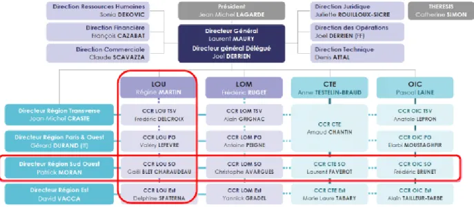
Figure 2: Organization of Thales Services 1.1.2. Flight Dynamics Department

Inside Thales Service, the departments are divided into a matrix organization considering the geographic area and the orientation of the activity.

The internship has been done in the Flight Dynamics Department in Toulouse, which is part of Division South-West, inside the User-Oriented Software Unit (LOU).

Figure 3: Internal organization of SSE units in Toulouse.

The Flight Dynamics department, as the name indicates provides services in the area of space mechan-ics, mainly to serve spacecraft operationâ ˘A ´Zs needs. In particular, the department provides two types of services:

(15)

1 INTRODUCTION 11 of56 • Technical support in the clientâ ˘A ´Zs facilities, concerning the areas of mission analysis, technical

studies,

• Software project development directly at Thales site, which includes in particular the development of software tools such as:

– CMS (Space Mechanic Center): Space Mechanics library used by CNES (for control opera-tions) and developed in FORTRAN. It includes the low-level libraries and high level services as maneuvers computations, guidance, orbit determination (OD), commands generation and so forth.

– PATRIUS: Analogue to CMS but developed in Java. - ZOOM : Orbit Determination toolkit developed for CNES - GOTLIB/PHRLIB (C++): Attitude Guidance Libraries.

– STELA: Long-term propagation tool developed for end-of-life activities

– GALILEO: Guidance library for the next generation European navigation system – ASPROSH: Commands Validation Library

– TAS: On-board orbit determination studies.

– COSMEUS (JACK, JMAN, JPOD, JPAD): Software suite for space mechanics.

1.2. General presentation

The present internship has been part of the project COSMEUS. In this section, an overview of the project and the software suite is proposed as well as a description of the considered topic during the internship. In a second moment, the planning followed during the internship and the educational purposes are exposed.

1.2.1. Description

General context. As mentioned previously, the internship I have done from July 2015 to December 2015 is a part of the development of the software suite COSMEUS (Complex Space Mechanics Utilities and Software), a JAVA library related to space mechanics which is composed of the following modules:

• JACK (Java Aerospace Capitalization Kit): low-level library for space mechanics (orbit propagation, force models, orbital event management, orbital parameter computation, â ˘A˛e);

• JUDE (Java Utilities for Development): library for exception, message, logs management; • JSCAR (Java Software for Comparison, Analysis and Reporting): library for tests; • JMAN (Java Maneuver): library for maneuver computation.

• JPOD (Java Precise Orbit Determination) and JPAD (Java Precise Attitude Determination): generic library for orbit and attitude determination.

• Other modules:

– JERY: Java Earth Reentry: library for atmospheric reentry

– JDEB: Java Debris: library for debris trajectory propagation and assessment of collision risks. The main result of the internship is to complete the existing software with functionalities related to the computation of maneuver with low-thrust engines.

(16)

1 INTRODUCTION 12 of56 Topic and internship purposes. During a space mission for a satellite for example, a large time is spent to operate the satellite. There are not only the operations to execute the actual mission: observation, telecom-munication, scientific experiments â ˘A˛e but also the operations to raise or maintain the satellite on the right configuration to achieve the mission. Among the second types of operations, there are the orbital maneuvers on which the internship is focused. Four types of orbital maneuvers exist:

• Orbit raising and early orbit phase: from the parking orbit where the satellite is launched, one or several maneuvers are required to reach the operational orbit.

• Station-keeping: once the satellite is on its mission orbit, the orbit is perturbed and maneuvers are required to maintain the satellite inside a given window.

• Debris avoidance: in the near-Earth area, hundreds of thousand of debris, resulting of the past launches and collision, or off-service spacecraft, are orbiting. Maneuvers are needed to avoid a colli-sion with one of those debris, which could damage the operated satellite.

• Interplanetary transfers: to reach the Moon or another planet of the solar system, a series of ma-neuvers is required.

The internship has been focused only on orbit raising maneuvers. To perform these, two types of propulsion are mainly used: the chemical and the electric propulsion.

Since the 1970s, while the chemical propulsion has been used for orbit raising, the technology of electric propulsion has been widely used in space technology to maintain the satellites on orbit. In 2003, Smart-1 lunar probe, which reached the Moon in 5000 hours with 80 kilograms of xenon gas, showed that electric propulsion could enable to reach high altitude orbits, and even liberate a spacecraft from the Earth gravity field. Since then electric propulsion has been of interest for industries. In the beginning of the year, the first commercial all-electric satellite was launched and the first European electric satellite are planned to be launched in 2017.

Indeed, the main advantage of electric propulsion is the ability to perform a maneuver such as orbit rising by consuming little propellant. For example, for typical chemically-propelled satellite, the amount of propellant used for orbit raising represents 55 % of the initial mass, while it represents only 20 % of a all-electric satellite. Hence, lighter satellites can be launched for the same payload, which reduces considerably the cost of launching. However, the main drawback is that the duration of maneuver is much longer: few months instead of few days for chemical satellite. In spite of this, it is likely that 20 % of launched satellites will be all electric in the near future.

In the software suite COSMEUS, the module JMAN provides the high-level functions to compute ma-neuvers that use chemical engines while the module JACK provides the classes to handle the low-level functions such as the maneuvers in the orbit propagation. For that, a maneuver is modeled as a sequence of impulsive thrusts, whose values and direction are computed at an optimal position on orbit. The main purpose of this project is to complete JMAN and JACK in order to integrate the electrically propelled ma-neuvers. Because the hypothesis of impulsive maneuver is not satisfied any more in the case of electric propulsion, the computation of the maneuver needs a global approach that aims to determine the values and directions of thrust at each time over a given period of time. For that, the theory of control and in particular the optimal control theory provides the tools to optimize the maneuver.

This master project presents two main aspects which will be developed in the report: the software engineering in particular the development of software from the expression of the needs to its final validation, and the application of the optimal control theory to a low-thrust maneuver problem.

(17)

1.2.2. Planning

The internshipâ ˘A ´Zs planning followed the typical development cycle used by the teams of the Flight Dy-namics department. The V-model illustrated in Figure4is applied in the department of Flight Mechanics and the internshipâ ˘A ´Zs planning may be divided into its five steps. In parallel, at each phase, documents are edited in order to keep the track of the development. The details of each phase will be presented in Section 4.

Figure 4: Description of V-model

1.2.3. Educational purposes

The final year internship is the first step towards the professional life and engineering work. As such, this is the opportunity to apply the knowledge acquired in class to practical problems and to learn how to adapt to a professional environment. The following points give the targets of the internship.

1. Technical level:

• Apply the technical knowledge learnt during the studentâ ˘A ´Zs studies, in particular in computer science and coding (JAVA, UML â ˘A˛e), in mathematics (algorithm used in resolution of optimal control problems and convergence) and space dynamics;

• Acquire new knowledge in software development;

• Adapt oneself to the existing tools and reuse them: development environment (Eclipse, Maven, SVN, quality software â ˘A˛e), libraries management, â ˘A˛e

(18)

1 INTRODUCTION 14 of56 2. Organizational level:

• Manage time organization to provide information and results to the company in due time; • Conduct a bibliographic research about the topic via Internet and the available books;

• Rapidly understand the guidelines of the project and its potential advantages and drawbacks for the given problem;

• Use the company resources (development environment, software â ˘A˛e) 3. Relational level:

• Discover the engineersâ ˘A ´Z way of working and the company philosophy;

• Exchange with the members of the Flight Dynamics department in order to understand the different projects;

• Contribute to the company functioning by presenting results by the end of the internship; • Be able to argue oneâ ˘A ´Zs results and choices throughout the internship.

(19)

2 THEORETICAL CONSIDERATIONS 15 of56

2. Theoretical considerations

This section will elaborate on the theoretical elements on which the project is based. To start with, the equations to model the motion of a spacecraft around the Earth are described. Secondly, is presented the state-of-the-art of applications of optimal control to the low-thrust problems in space mechanics. Finally, the principle of the homotopy continuation methods is explained.

2.1. Two-body problem and perturbations

In orbital maneuver, the motion of the spacecraftâ ˘A ´Zs center of gravity is studied. In first approximation, the two-body problem is a good model to describe the motion in the near Earth space. In this section, this model will be presented as well as the perturbations of this model, which justify the need for maneuvers to correct the orbit.

F= −µEarth

m

||r||3r (1)

with µEarth the Earth gravitational constant, m the spacecraft mass and ~r the position vector.

The dynamic of the spacecraft is then described by: ¨r= −µEarth

||r||3 r (2)

The analytic resolution of Equation (1) gives the three Kepler laws of planetary motion. Originally, these laws are meant to describe the motion of the planets around the Sun; nevertheless, the results can be transposed to the motion of a spacecraft around the Earth.

1st law. The trajectory of the spacecraft is an ellipse, whose one of the foci is the Earth.

2nd law. A line joining the spacecraft and the Earth sweeps out equal areas during equal intervals of time. 3rd law. The square of the orbital period of the spacecraft is proportional to the cube of the semimajor axis of its orbit.

An elliptic orbit can be entirely described if 6 independent parameters are known. There are different types of parameters among the Keplerian parameters, the equinoctial parameters and the Cartesian parame-ters.

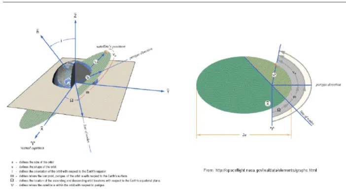
Keplerian parameters. Derived from the resolution of the two-body problem, the Keplerian parameters, defined in Figure 5, allow defining the shape of the ellipse, its orientation in 3-dimensional space and the position on orbit. On one hand, a position on the orbit is entirely characterized in the orbital plane by 3 parameters: the semi major axis (SMA), the eccentricity and the true anomaly . The three other parameters permit to characterize the orbital plane with respect to a reference plane: the equatorial plane. The inclination is the angle between the reference plane and the orbital plane. The right ascension of the ascending node (RAAN) angle represents the angle between the vernal axis and the ascending node axis. Finally, the argument of perigee is the angle in the orbital plane between the ascending node axis and the direction of the perigee.

(20)

Figure 5: Description of the Keplerian parameters

Equinoctial parameters. In the case of circular orbits (e ≈ 0) or equatorial orbits (i ≈ 0), the Keplerian parameters are not necessarily defined (for example, the argument of perigee for a circular orbit can be any value between 0 and 2π). Consequently, the orbit is characterized by the 6 equinoctial orbital parameters: p, f, g, h, k and L, which can be expressed with the Keplerian parameters.

p=a(1 − e2) (3) f =ecos(ω + Ω) (4) g=esin(ω + Ω) (5) h=tan(i 2)cos(Ω) (6) k =tan(i 2)sin(Ω) (7) L=ω + Ω + ν (8) (9) Cartesian parameters. The position of the satellite on its orbit may also be expressed in terms of position r and velocity v vectors in a Cartesian frame.

In the orbital plane, the unitary vector ~Pis defined by A~

|| ~A||, where ~Ais the vector oriented towards the

perigee from one of the focus of the orbit. Let ~Qbe the vector perpendicular to ~P, corresponding to a true anomaly of 90 degrees. In the frame (~P, ~Q), both the position and the velocity vectors are expressed by:

~r =x~P + y ~Q (10)

(21)

2 THEORETICAL CONSIDERATIONS 17 of56 with,

The vectors ~Pand ~Qcan be expressed in an inertial geocentric frame by using the Keplerian parameters:

2.1.1. Perturbations

In the previous section, the Keplerian motion has been presented. In reality, the spacecraft is not only af-fected by the Earth gravitational field. In this section, the other forces that perturb the motion are introduced. The first origin of perturbation is the Earth shape. Indeed, the expression of the gravitational forces presented above is verified if the Earth is perfectly spherical, and uniformly dense. Because the Earth is actually alike an ellipsoid, the gravitational force is expressed by an expansion in spherical harmonics that characterize the effects of the Earth flatness and the tidal deformation. The spacecraft can also be affected by the other bodies of the solar system, in particular the Moon and the Sun. All these possible gravitational contributions are added in the right term in Equation (1).

The second type of perturbation is due to the atmosphere. Although at the orbital altitudes the atmo-sphere is nearly nonexistent, the atmospheric drag cannot be neglected in certain cases, for instance in LEO. Thus, in Equation (1), a force opposed to the velocity and proportional to the spacecraft surface and its drag coefficient is then added.

The last significant perturbation is caused by the solar radiation. A pressure force appears due to the exchange of quantity of motion between the photons and the spacecraft. This force is proportional to the spacecraftâ ˘A ´Zs surface, its reflectivity coefficient and the solar radiation pressure per surface unit.

All these forces perturb the Keplerian motion presented in the previous section. This is why the orbital maneuvers performed by chemical or electric engines are necessary to place or maintain the spacecraft on its mission orbit. In the case of electric propulsion, it can be described the relation between the time variations of the orbital parameters and the external forces via the 6 Gauss equations. The forces (perturbation and thrust) are usually expressed in the RTN frame. As illustrated in Figure 6, it is a local frame whose R-axis is along the Earth-Spacecraft unit vector, the N-axis is along the angular momentum vector (normal to the orbital plane) and the T-axis to form a right-hand frame.

Figure 6: Description of RTN frame

There are many manners to express the Gauss equations. If they exist for the Keplerian parameters, the equinoctial parameters are usually used to compute low-thrust maneuver. In addition to allow the definition

(22)

2 THEORETICAL CONSIDERATIONS 18 of56 of orbital parameters for singular orbits, the time variations of equinoctial parameters avoid numerical singularities, in particular the division by zero. This is why they are widely used to formulate the optimal control problems associated to the computation of low-thrust maneuvers.

2.2. Generalities about nonlinear optimal control

As said previously, the computation of maneuver using electric propulsion differs from the computation of chemical maneuver by the thrust model. . Indeed, the profile of chemical thrust is so compressed in time and the amplitude of thrust so large that it can be modeled as an impulse. Hohmannâ ˘A ´Zs work has described the optimal trajectory, the optimal delta-v and the optimal position to perform the maneuver, in order to modify an orbit.

On the contrary, because electric propulsion provides low thrust, the duration of a burn is much longer such that it must be modeled as a continuous pulse. As a consequence, the computation of a maneuver should adopt a global approach, that is to say the control law must be determined at each time of the maneuver this is why the optimal control theory is used in this case.

In control theory, this is the branch which studies the control of dynamical systems minimizing or maximizing a given performance, with respect to any constraints. Since the early 2000s, many studies have been done on the application of optimal control to the low-thrust maneuvers and nowadays, it still is a moving branch of research. In this section, a general formulation of an optimal control problem is presented as well as the main approaches to solve such a problem illustrated by applications in aerospace.

2.2.1. General formulation

Any optimal control problem can be formulated generally as following.

Let be a system whose finite state x(t) is to be controlled by a law u(t) . The dynamics of the state is then described by the equation:

˙

x(t)= f (t, x(t), u(t)) (12)

Both the initial and the final state are known and noted by x(t0) = x0, x(tf) = xf, whereas the control

law u(t) must be determined. Let be C(tf, u) the cost function to optimize defined by the general expression:

C(tf, u) =

Z tf

t0

L(x, x(t), u(t)) dt+ ψ(tf, xf) (13)

, with L a C1function called the cost rate and ψ a C0function corresponding to the final cost.

2.2.2. Methods of numerical resolution

In the scientific literature, many methods are mentioned to solve a problem of optimal control. They can be sorted into 3 main approaches illustrated in Figure7. The following sections will present each of them and their applications to aerospace extracted from [1].

Dynamic programming. The first method, the dynamic programming, provides a closed-loop control. The principle consists in the iterative resolution of the problem from the final time. At each time, all possible states are considered and the jump from one state to another is associated to a certain cost, depending to the previous and next states and a given decision, for example switch the engine on or not. The optimal solution is given by following the path with the lowest total value. The main advantage of dynamic programming is

(23)

Figure 7: Overview of methods in optimal control

the guarantee to obtain a global solution. They are barely used for the computation of the orbital maneuver because, the computation of the maneuver involves the reaction of perturbations, which is not known a priori; the considered control is an opened-loop control and therefore is out of the scope of this method. Direct methods. Another type of methods to solve an optimal control problem is the direct methods also called â ˘AIJfirst-discretize-then-optimizeâ ˘A˙I methods. They are based on the transcription of the problem into a finite-dimension non-linear programming (NLP) problem through the discretization of the state vector and the control. The two subtypes, the sequential and the simultaneous methods, differ from the way to perform the discretization. Indeed, in the simultaneous methods, both the state vector and the control are discretized, whereas in the sequential methods, only the control is discretized and the dynamics is embedded in the NLP problem.

The optimal solution is computed to verify the KKT (Karush â ˘A ¸S Kuhn â ˘A ¸S Tucker) conditions for optimality.

The advantages of these approaches are the ability to easily integrate constraints on the state and control vectors and the convergence of the algorithm. However, the obtained precisions are rather low for aerospace uses. Moreover, the dimensions of the problem could be very large and could be time consuming even if there are various efficient open-source routines such as IPOPT in C++. It has to be noted that the solution could be non-smooth.

In [2], a simultaneous method is implemented using a direct transcription for the state vector and the control of low-thrust maneuver and direct collocation to solve the NLP problem. The search space includes about 600 000 variables and constraints, and the solution given in the article has needed 3775.31 seconds (around 1 hour).

Indirect methods. The last available approaches are the indirect methods, as known as â ˘ AIJfirst-optimize-then-discretizeâ ˘A˙I methods. In opposition to the direct methods, the principle is to find necessary conditions of optimality before discretizing the problem. As described in [1] and [3], the calculus of variations and the

(24)

2 THEORETICAL CONSIDERATIONS 20 of56 Pontryagin maximum principle are two means to obtain the conditions of local optimality, which are then reduced to a boundary-value problem solved by a shooting method to find a root of a certain function.

Research works in aerospace and spatial field commonly favor these types of methods due to high accuracy and the smoothness of the solutions. However, the indirect methods present drawbacks. Indeed, they are usually quite complex; there is no guarantee to find a global solution and the convergence of the shooting methods is hard to reach because of the nonlinearity of the problem and the sensitivity to the initial guess. This is why they are generally coupled to direct methods or global optimization techniques to cope with the difficulties of the indirect methods. For instance in [4], the authors try to find a good initial guess by a resolution beforehand that uses a direct method, which initializes the shooting method.

An indirect method will be used in JMAN for the aforementioned advantages. As for the difficulties in initializing the shooting method, homotopic methods have been used. The principle of this type of methods is detailed in the next section.

2.3. Homotopy continuation methods

During the internship, homotopy continuation methods have been used to solve the difficulties mentioned in the previous section. In this section, they will be presented in a generic form.

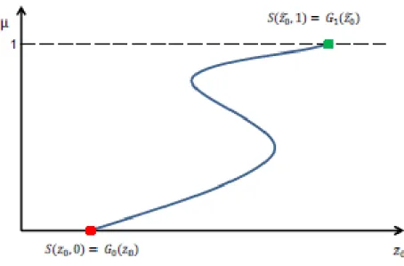
In topology, homotopy is the concept of deforming one space into an other one in a continuous manner. The homotopic methods use this idea to solve difficult problems. The principle of these methods is to solve a difficult shooting problem, noted A, using an easier shooting problem B. Let be G1(z) the shooting function

of the problem A, and G0(z) the shooting function of the problem B and z0its root (or one of its roots).

A continuous homotopy function is then defined to connect the two problems by

S(z, µ)= µG1(z)+ (1 − µ)G0(z) (14)

, with the parameter of homotopy which permits to relate the two problems. When the parameter of homo-topy µ is equal to 0, the problem B is recovered while the initial problem A is associated to µ= 1. Figure8 illustrates an example of zero-path with a one-dimensional variable.

(25)

2 THEORETICAL CONSIDERATIONS 21 of56 There are different ways to perform the zero-path tracking. Two of them have been used during the internship for the two types of problems mentioned in the report. The first resolution consists in using a heuristic about the two variables (z, µ) to predict the next step in the path-tracking. The details of its application to the first type of problems will be presented in Section 3.2.2. The second resolution exposed in Sections 3.1.4 and 3.2.3 is based on the integration methods, for instance the prediction-correction method.

(26)

3 LOW-THRUST MANEUVER PROBLEMS AND RESOLUTIONS 22 of56

3. Low-thrust maneuver problems and resolutions

In this section, we will first elaborate on the application of the conditions given by the Pontryagin minimum principle to two types of problems related to the computation of low-thrust maneuver: the minimization of the maneuver duration and the problem that consists in minimizing the fuel consumption. It will be shown that each of the corresponding optimal control problems can be reduced into one Two-Point Boundary Value Problem (TPBVP), that is to say a set of differential equations with initial and final boundary conditions. The numerical methods to solve such problems using a Newton-type method will then be presented.

3.1. Conditions of optimality

3.1.1. Pontryagin minimum principle

As mentioned previously, the indirect method will be used and the necessary conditions of optimality are derived from the Pontryagin minimum principle.

By using the notations introduced in Section 2.2.1, the Hamiltonian function is defined by:

H(t, x, u, λ)= L(t, u(t) + λTf(t, x(t), u(t)) (15) , with λ the vector of the costate related to each component of the state vector.

Pontryagin minimum principle. Let u∗(t) be an admissible optimal control law, and x∗(t) the optimal trajec-tory associated to the state dynamic and to u∗(t), then it exists a vector λ∗(t) such that

˙x∗(t)=∂H ∂λ(t, x ∗_{, u}∗_{, λ}∗ ) (16) ˙ λ∗ (t)= − ∂H ∂x(t, x ∗_{, u}∗_{, λ}∗ ) (17) H(t, x∗, u∗, λ∗)= min u H(t, x ∗_{, u, λ}∗₎ ₍₁₈₎

The superscript â ˘AIJstarâ ˘A˙I notes the optimal variables.

3.1.2. State dynamic

The first step in the formulation of the problem is the definition of the state vector x. In both types of problems considered in the report, the state vector is composed of the Cartesian coordinates of the position and the velocity vectors presented above and the spacecraft mass.

The dynamics of the state vector is derived from the second Newton law and the definition of the specific impulse. ˙r(t)=v (19) ˙v(t)=Fext+ Tmax u(t) m(t) (20) ˙ m= − Tmax ||u(t)|| Ispg0 (21) , with

(27)

3 LOW-THRUST MANEUVER PROBLEMS AND RESOLUTIONS 23 of56 • r the position vector,

• v the velocity vector,

• Fextthe vector of the perturbation forces,

• Tmaxthe maximal thrust provided by the spacecraft’s engines,

• m the spacecraft mass,

• u(t) the thrust vector in the RTN frame at time t, • Ispthe specific impulse,

• g0the gravitational acceleration at sea level. 3.1.3. Time optimal problem

The problem that consists in minimizing the duration of the maneuver is characterized by the following cost function:

C(tf, u) =

Z tf

t0

dt= tf − t0 (22)

For the problem, the control law u is expressed by u= T(t)α(t), with T(t) the amplitude of the thrust and α(t), the unit vector giving the thrust direction.

Besides, this type of problem is an end-time free problem, so the final time tf which is unknown must

appear in the state vector, and the equation of its derivative ˙tf = 0is added to the state dynamics Equations

19,20and21.

The Hamiltonian function is then:

H= 1 + λrv+ λv(Fext+ Tmax u(t) m(t)) −λm(Tmax ||u(t)|| Ispg0 )+ λtf(0)+ γ(1 − ||α(t)|| 2₎ with,

• γ , the function that constrain the direction vector to be unitary. It is defined by γ (

= 0 , ||α(t)||2 _{= 1}

≤ 0 , otherwise • λr, λv, costate vectors associated to the position and velocity vectors

• λm, costate variable associated to the mass

• λtf, costate variable associated to the final time

The Pontryagin minimum principle is then applied. The Hamiltonian function should be minimized hence the optimal direction vector is a solution of

∂H ∂α =λr T(t) m(t)− 2γα= 0 ⇒ α ∗ ∝λv

The control α is constrained to be unitary, it comes α∗= λv

(28)

3 LOW-THRUST MANEUVER PROBLEMS AND RESOLUTIONS 24 of56 The Hamiltonian function is linearly dependent on the value of the thrust T (t), hence the status of the thrust is a bang-bang law controlled by a switching function ϕ(t)

∂H ∂T = ||λv|| m(t)− λm Ispg0 = ϕ(t) (23) It comes T(t)=          0 , ϕ(t) < 0 1 , ϕ(t) > 0 0 < T < 1 , ϕ(t) = 0 (24)

The dynamics of the costate variables is then written by deriving the Hamiltonian and replacing the expression of the control:

˙ λr= −λv ∂Fext ∂r , ˙λv = λr, ˙λm= ||λv|| T(t) m2 (25)

The sets of differential Equations19,20,21and25are completed by boundary conditions on the states and the costates summarized in Table 1. These conditions are given by the relationship of the known variables and their associated costates. Indeed, because the state vector is known at the initial and the final times, the corresponding costates are free. In opposition, because the final time is unknown, there is a condition on λtf, which is dependent the part of the cost function related to the final state ψ(xf, tf) = tf.

Similarly, because the final mass is also unknown, there is a condition on the value of the final mass costate variable λm(tf).

Table 1: Boundary conditions and conditions of transversality (time-optimal)

x(t0)= x0 λr(t0), λv(t0) are free x(tf)= xf λr(tf), λv(tf) are free m(t0)= m0 λm(t0) is free m(tf) is free λm(tf)= _∂m∂ψ = 0 tf is free λtf = ∂ψ ∂tf = 1

As a result, the time optimal problem formulated by the application of the Pontryagin minimum princi-ple has been reduced to a TPBVP, which must be solved.

3.1.4. Mass optimal problem

The second type of problem considered consists in minimizing the fuel consumption or equivalently max-imizing the final spacecraft mass for a given initial and final time. The cost function is then expressed by

C(tf, u) = −m(tf)= −m0−

Z tf

t0

˙

m(t) dt (26)

From the set of equations (2) describing the state dynamics, minimizing the fuel consumption is equiv-alent to minimizing the amplitude of the control ||u||.

The cost function can be expressed by:

C(tf, u) =

Z tf

t0

(29)

3 LOW-THRUST MANEUVER PROBLEMS AND RESOLUTIONS 25 of56 In this case, the Hamiltonian function is then:

H= ||u(t)|| + λrv+ λv(Fext+ Tmax

u(t) m(t)) −λm(Tmax ||u(t)|| Ispg0 )+ λtf(0)

The Hamiltonian function is linearly dependent on the control u(t). A situation similar to the time-optimal problem brings to a bang-bang control, and hence to a discontinuous control. Nevertheless, con-trary to the time-optimal problem, the engines are not necessary â ˘AIJonâ ˘A˙I during the entire maneuver, the structure of the control, in particular the number of the switch on/off, needs to be known during the resolution.

In [5], the authors suggest the use of a homotopy method using the problem of minimizing the energy. For this problem defined the cost function is then chosen to be

C(tf, u) = Z tf t0 1 2||u(t)|| 2_dt ₍₂₈₎

The corresponding Hamiltonian function is H= 1 2||u(t)|| 2_{+ λ} rv+ λv(Fext+ Tmax u(t) m(t)) −λm(Tmax ||u(t)|| Ispg0 )+ λtf(0)

As mentioned in the article, the Hamiltonian allows avoiding a discontinuous control. Indeed, in the present case, the derivative of the Hamiltonian with respect to ||u|| is still dependent on the control, and as what follows shows, the optimal amplitude of thrust is continuous.

∂H ∂||u(t)|| =||u(t)||+ ||λv|| m(t)) − λm Ispg0 ⇒ ||u(t)||∗= −||λv|| m(t)+ λm Ispg0

The idea is then to deform the solution given by the energy-optimal problem to reach the solution of the mass-optimal problem. To connect the two types of problems, in [5] and in [6], two criteria are mentioned: the power criteria and the convex criteria. During the internship, the convex criterion has been chosen because of the regularity of the zero-path which is supposed to be followed. Indeed, the cost function is

C(tf, u) = Z tf t0 µ ||u(t)|| +1 2(1 − µ) ||u(t)|| 2_dt ₍₂₉₎

It can be verified that when µ, parameter of homotopy, is equal to 0, the problem minimizes the energy and when µ is equal to 1, the problem minimizes the mass.

The Pontryagin minimum principle is then applied to the following Hamiltonian function

H= µ ||u(t)|| +1 2(1 − µ) ||u(t)|| 2_{+ λ} rv+ λv(Fext+ Tmax u(t) m(t)) −λm(Tmax ||u(t)|| Ispg0 )+ λtf(0)

(30)

3 LOW-THRUST MANEUVER PROBLEMS AND RESOLUTIONS 26 of56 The unconstrained amplitude of the control law||u(t)|| verifies:

∂H ∂||u(t)|| =µ + (1 − µ)||u(t)|| + ||λv|| m(t)) − λm Ispg0 ⇒ ||u(t)||∗= −Tmax||λv|| m(t) + Tmax λm Ispg0 −µ 1 − µ

The optimal thrust direction is still proportional to the costate vector λv.

Because the amplitude of the control is normalized by Tmax , it must be between 0 and 1. Hence the

control law becomes:

u(t)=            0 , ||u(t)||∗< 0 ||u(t)||∗ λv ||λv|| , 0 < ||u(t)|| ∗_{< 1} λv ||λv|| , 1 < ||u(t)|| ∗

It can be verified that the control is continuous.

The derivation of the Hamiltonian with respect to the states gives the following dynamics of the costate variables with the control u(t) as defined previously.

˙ λr= −λv ∂Fext ∂r , ˙λv = λr, ˙λm= ||λv|| Tmax||u(t)|| m2 (30)

In the same manner that the boundary conditions are determined for the time-optimal problem, the sets of differential equations19,20,21and30are completed with the boundary conditions given in Table2. For the mass-optimal problem, the part of the cost function related to the final state is ψ(xf, tf)= −m(tf).

Table 2: Boundary conditions and conditions of transversality (mass-optimal)

x(t0)= x0 λr(t0), λv(t0) are free

x(tf)= xf λr(tf), λv(tf) are free

m(t0)= m0 λm(t0) is free

m(tf) is free λm(tf)= _∂m∂ψ = 0

Similarly to the time-optimal problem, the mass-optimal problem can be solved by using the TPBVP composed of the state and costate dynamics and the previous boundaries conditions. It must be noted that the TPBVP is dependent on the parameter of homotopy, and the resolution of the mass-optimal problem needs to find a numerical series of parameters of homotopy that converges towards 1.

3.2. Numerical resolution of TPBVP: Indirect Single Shooting Method

In the previous section, it has been shown that the optimal control problems related to the computation of orbital maneuvers can be reduced into TPBVP. Within the scope of the internship, an indirect shooting method has been chosen because there is no need of an a priori knowledge of the structure of the control. Indeed, the TPBVP is reduced to a shooting function G(z) whose dynamics is given by the differential equa-tions of the state and costate vectors, and its final and final values related to the boundaries. The principle is to â ˘AIJshootâ ˘A˙I from an initial point z0and to iterate until the final value converges to its targeted values.

Consequently, the problem is solved for the costate variables, in other words, because the dynamics of the costate variables is known, the unknown of the system are actually p0= (tf, λr(t0), λv(t0), λm(t0), λtf(t0) for

(31)

3 LOW-THRUST MANEUVER PROBLEMS AND RESOLUTIONS 27 of56 algorithm is illustrated in Figure9. The resolution of the TPBVP is then equivalent to find a root of the shooting function G(z).

Figure 9: Indirect Shooting Method

3.2.1. Root finder algorithms

Newton method and variants

. To find the root of a function, the Newton method is widely used to find the roots of a real function of one variable and can be easily generalized to multivariate vector function. Let be G(z) a multivariate vector real function. The first-order Taylor expansion around a given point z0is

G(z0+ ∆z) ≈ G(z0)+ dG(z0)∆z + o(||∆z||)

, with dG(z0) the Jacobian matrix is estimated at point z0. If z1 = z0+ ∆z is close enough to a root z0

then

G(z0)+ dG(z0)∆z ≈ 0 ⇒ ∆z = dG(z0)−1

From the previous equation, an iterative method is designed to find a root of G(z).

The first issue of this method is the estimate of the Jacobian matrix. Indeed, for a nonlinear function whose analytic expression is unknown, a manner to have a good estimate is to approximate the derivative with finite differences

dG(z0) ≈ (Gi(z+ hj) − Gi(z))

1 h

(32)

3 LOW-THRUST MANEUVER PROBLEMS AND RESOLUTIONS 28 of56 ,with

• Gi the real function corresponding to the ith coordinate,

• hjthe vector with the jth coordinate equals to h, and 0 elsewhere

The disadvantage of this method is the number of the function evaluation which can be huge for large dimensions.

Another manner to estimate the Jacobian matrix has been investigated: the Broyden approximation. The principle is to compute good approximation by finite differences just once and then the Jacobian matrix is updated using a first-order approximation as mentioned in [7,8].

Direct search method

. Because of the given problem is highly nonlinear, a direct search method has been considered such as the use of an optimizer to approach a root of the shooting method. Indeed, the principle is to minimize a positive real objective function related to the vector shooting function in order to get a solution close to a root.

Among the available optimizers, the simplex optimizer has been used. The principle of this type of optimization is to evaluate the multivariate objective function at the vertices of a simplex, which is updated at each iteration. This optimizer has several interesting advantages for the considered problem. The algorithm provides a global optimum without using the derivatives of the function. It must be mentioned that there are other types of direct search method such as CMAES (Covariance Matrix Adaptive - Evolution Strategy) optimizer which is a stochastic method commonly used for the global optimization of non-linear functions. Usually, the latter gives results faster and is more reliable than the deterministic optimizers; however, it can be slower when the dimension of the problem is smaller of around 10.

3.2.2. Resolution of the time-optimal problem by homotopy on the maximum thrust

The shooting method will be applied to the following function:

The value of the function is computed after integration of the differential equations19,20,21and25. One of the difficulties of the application of the shooting method to solve a TPBVP is the initialization of the unknown parameters. Indeed, a shooting method converges when the initial point is close to the optimal solution. Another difficulty is about the optimality of the solution when it is found. Indeed, the Pontryagin principle gives only conditions for local optimality. Moreover, although the Newtonâ ˘A ´Zs method gives accurate solution when initiated close to a root, it only gives a local solution. Consequently, the algorithm described above must be completed to guarantee to find a global optimum. A continuation homotopy method has been used.

In [9], the authors mentioned the same difficulties in initializing the indirect shooting method and sug-gest the use of a continuation method on the maximum thrust Tmax. Indeed, the problem seems to be easier

to solve for higher thrust. In the article, it is demonstrated that the function giving the final time is contin-uous with Tmax; consequently, a homotopy on this parameter is possible. Besides, a heuristic is highlighted

(33)

3 LOW-THRUST MANEUVER PROBLEMS AND RESOLUTIONS 29 of56 which relates the maximum thrust and the final time. Based on the fact that the higher the maximum thrust the faster the maneuver is performed. Consequently, a heuristic formulated by a constant value of the prod-uct of these two quantities Tmaxt − f ≈ cstis considered. In the article, the constant is shown to be related

to the initial and final orbital parameters and the initial spacecraft mass.

Figure 10: Homotopy on thrust

Because of the simplicity of implementation, this method has been chosen and introduced in the compu-tation of maneuvers in JACK and in JMAN. The procedure is illustrated in Figure10. After an initialization of the costate vector with zeros and the maximum thrust set at a high value (order of tens of Newton), the shooting problem is solved for the optimal final time t∗_f and for the optimal costates vector p∗_O. The maxi-mum thrust is then updated for the next iteration. In JACK, it has been chosen to use a geometric series that allows a fast convergence to low values. As for the costates vector, it updated with the optimal vector found at the previous iteration. The final time tf is updated by:

tf, n+1=

Tmax, n

Tmax, n+1

t∗_{f, n}

3.2.3. Resolution of the mass-optimal problem

Similarly to the resolution of the time-optimal problem, a shooting function for the mass optimal problem is defined by:

The value of the function is computed after integration of the differential equations19,20,21and30. As mentioned in Section 3.1.4, the resolution of the mass-optimal problem is based on a homotopy to use an easier problem, the energy-optimal problem. The resolution starts with the determination of the optimal solution z0 of the problem of energy-optimal by using a classic shooting method. Due to the type

(34)

3 LOW-THRUST MANEUVER PROBLEMS AND RESOLUTIONS 30 of56

The following explanation is illustrated by Figure 11 and Figure 14. The path-tracking algorithm is initialized by this optimum. In JMAN, the path-tracking is performed by a prediction-correction method. Until the parameter of homotopy Î˙z reaches a value close to 1, a prediction is determined by using a classic integration method such as an Euler prediction, which uses the tangent vector to the curve at the current point represented by the green arrow in Figure14.

Added to the current point, it comes the point (z, µ), which is not necessarily a zero of S (z, µ) but is close enough to a zero to allow the convergence of the shooting algorithm by zero finding method. The correction phase consists in getting closer to the zero-path.

(35)

4 DEVELOPMENT OF THE MODULE 31 of56

4. Development of the module

Seeing as the final aim of the internship is to complete an existing software suite with new functionalities, the steps of the software development have been followed, in this case, those of the V-model. This section will introduce each of them as well as will describe how they have been applied to the project.

4.1. Analysis of needs and expression of requirements

During the development of software, the analysis of the needs is the very first step. Indeed, the client usually expresses a list of functionalities that the software shall do. That allows in particular for the clients and the engineers to agree on the final characteristics of the software. For the internship, as the product is meant to be used internally, this phase belongs to the team of the department.

Once the list established and the functionalities ensured to be implemented in the product, these func-tionalities are then translated as services, requirements and input/output lists and written in the SRS (Soft-ware Requirements Specifications) document.

4.1.1. Functionalities for maneuver computation

After the first phase of bibliographic research and familiarization with the development environment and the existing software, the first step of my work was to list all functionalities necessary in JACK and JMAN modules for orbit maneuver computation, in particular in the case of non-impulsive maneuvers. All these functionalities were then sorted into categories that constitute the main aspects of the computation of ma-neuver: mission, constraints, criteria, maneuver model, effective maneuver, correction and optimization. At the end of this phase, a synoptic has been edited (Appendix 1: Thematic synoptic)

The category â ˘AIJmissionâ ˘A˙I includes all possible mission types (early orbit phase, station keeping, interplanetary transfers, collision avoidance and end of life), the type of satellite formation (unitary, forma-tion flying or constellaforma-tion), and the opforma-tions for each mission type. In the early orbit phase, for instance, the maneuver can be performed as soon as possible, as late as possible before a given date or by minimizing the delta-v.

The category â ˘AIJconstraintsâ ˘A˙I handles the different constraints that the module should take into ac-count during the computation of a maneuver including the mission constraints, the engine operation con-straints and the overall satellite concon-straints. To these, it has been added the environmental factors. These latter are not actually constraints but the causes of constraints that must be handled such as the eclipses, the Van Allen belt or the South Atlantic anomaly.

The category â ˘AIJcriteriaâ ˘A˙I considers the types and the parameters to define a window during the computation of a station-keeping maneuver.

Since the maneuver has to be modeled, the next category, â ˘AIJmaneuver modelâ ˘A˙I, gathers all aspects of the model of a maneuver or a thrust. The first one is the type of maneuver. Indeed, during operations, several models are used. The commanded maneuver handles the maneuver without performance or real perturbation consideration. The observed maneuver is computed from the telemetry data, but without con-sidering the performances whereas the effective maneuver handles both the reality throughout the telemetry data and performances via models. In addition, there are the type of propulsion, the element of an actual maneuver (impulse, pulse and burn), the type and the model of thrust among others.

The category â ˘AIJeffective maneuverâ ˘A˙I gathers the tools useful for its determination: the model of the propulsion system, the calibration (link between the commanded efforts and the actually applied efforts), the measurement of the performance and the maneuver reconstruction (data processing, filters â ˘A˛e).

(36)

4 DEVELOPMENT OF THE MODULE 32 of56 The last category handles the tools for optimization such as the model and the definition of an optimal control problem and the methods for the numerical resolution.

4.1.2. Expression of the services and requirements

All these functionalities are expressed in a form of list in boxes; however, in order to design the software, they need to be expressed as services and requirements which will be regrouped in the SRS documents of JACK and JMAN. The two modules have distinct purposes, indeed JACK handles all low-level functions such as space dynamics, frame conversion, orbit propagation â ˘A˛e while JMAN handles all high-level func-tionalities: correction computation, correction strategy, type of mission â ˘A˛e At this steps, the functionalities are shared between the two modules following their own characteristics.

The service is the highest level of specifications and corresponds to a global functionality.

During the last internship, in JMANâ ˘A ´Zs SRS, the different types of mission have been taken into account to which it has been added the maneuver calibration and the maneuver reconstruction. In JACK, the definition and the resolution of an optimal control problem is added as a service.

The second level of specifications is the requirements, which are the basic functions needed to achieve a service. For example, in JMAN, there is the computation of a correction using the optimal control and in JACK, the required numerical resolution methods.

4.2. Architectural and detailed conception

4.2.1. Architectural conception

After writing the requirements, the architectural conception aims to integrate the basic functions, described in the requirement inside appropriate sets of JAVA packages and classes in the case of object-oriented programming. The main purpose of the internship was to complete the correction function in JMAN; therefore the conception phase will be illustrated through this example.

A package gathers all classes which ensure a more global function such as compute a correction, while a class object usually ensure one basic function such as compute one type of correction (eccentricity, semi ma-jor axis â ˘A˛e). Then inside the package â ˘AIJcorrectionâ ˘A˙I, to reduce the dependencies between the objects, an interface is used. All types of correctors should implement the same interface â ˘AIJICorrectorâ ˘A˙I and include certain functions. Another purpose of a good architecture is the code factorization; indeed, in case of redundant parts of code, they are usually gathered in an abstract class. In our example, because all cor-rectors have a type of correction which is characteristic of it, the getter of this attribute can be implemented in an abstract class. Therefore, all correctors extend from the abstract class

â ˘AIJAbstractCorrectorâ ˘A˙I. This architecture is inherited from the previous state of JMAN software, however, has been added the classes related to the maneuvers performed with electric engines.

The same work has been done for the part related to the optimal control in JACK. The subpackage â ˘AIJoptimizationâ ˘A˙I has been added in the package â ˘AIJmathâ ˘A˙I, to handle all classes to solve a generic optimal control problem.

4.2.2. Detailed architecture

The next step aims to design the architecture of the software by means such as UML diagrams: package, class and sequence diagrams. The detailed conception consists in summarizing the details of implementa-tion and the technical choice such as the algorithms in the Software Design Document (SDD).

(37)

4 DEVELOPMENT OF THE MODULE 33 of56 During this phase, the investigation to find the available algorithms that have been mentioned in the previous sections is done as well the definition of all functions.

4.3. Development and tests

The development is the actual phase when the implementation of the aforementioned classes and algorithm is done. This phase is also the opportunity to learn how to use some tools used in software development, especially the tools to handle the code versioning and a project composed by many modules. Indeed, during the internship, Subversion (SVN) was used to manage the different version of the codes while Maven was used to compile and manage the dependencies between all modules present in COSMEUS.

In JACK, the work consists in implementing the framework to handle the resolution of a generic optimal control and the algorithm for the numerical resolution (Newton method, shooting methods â ˘A˛e). Besides, the model for a continuous thrust has been added to be handled during the orbit propagation.

In JMAN, most of the work was the integration of the routines that performed the computation of low-thrust maneuvers in the actual architecture. For that, the classes to specify a time optimal problem and a mass-optimal problem are added in the architecture. Then it has been implemented the routines necessary for the computation of maneuvers, in particular the two homotopy algorithms.

In parallel to the development, the design of the tests has been done. Indeed, the tests are based on a set of unit tests to verify on one hand whether the functions and the algorithm are correctly implemented, and on the other hand to validate the results with respect to some reference software which will be presented in the next section.

4.4. Reference software and validation

The part of validation has involved two pieces of software developed as part of research work.

For the time-optimal problem, the open source software MIPELEC developed in FORTRAN by CNES [10] mid-2000s has been used as reference. Optimized for the medium and low-thrust orbit raising ma-neuver, MIPELEC is based on two techniques to cope the difficulties of the time-optimal problem: the averaging of the orbital parameters on one orbital period and a pre-resolution of the energy-optimal prob-lem to initialize the shooting algorithm. Indeed, because the low-thrust maneuver probprob-lem is â ˘AIJrapidly rotatingâ ˘A˙I; the averaging method allows eliminating the high-frequency oscillations of the parameters. As mentioned above, the energy-optimal problem is easy to solve and provides a good initial guess. The numerical resolution is then based on two existing routines for the numerical resolutions: NLEQ1 for the resolution of nonlinear problems and RKSUITE for the integration.

For the mass-optimal problem, the software MfMax developed by researchers from ENSEEIHT [11], an engineering school in Toulouse, has been used to generate reference results. Based on the mathematical FORTRAN routine HOMPACK90 for the homotopy and RKF45/HYBRD for the integration of the ODEs. It implements the resolution of the mass-optimal problem by the same homotopic continuation method as used in JMAN.

(38)

5 ENCOUNTERED PROBLEMS 34 of56

5. Encountered problems

The development of the modules JACK and JMAN has raised a certain number of questions concerning the optimal control and its numerical resolution. This section will summarize them and the solutions proposed during the internship.

5.1. Choice of the formulation of the optimal control problem

The very first question during the phase of conception is the choice of the orbital parameters used to formu-late the optimal control problem. Indeed, in the scientific literature, the equinoctial parameters are generally used for many reasons. First of all, the dynamics of this set of parameter is quite regular. When the eccen-tricity or the inclination is equal to zero, there are not singularities due to the division by zero. In addition, the implementation is easier because the initial and final boundaries are directly related to the state vector. This last point is interesting if the maneuver is performed without a rendezvous on orbit, in other words, when the final longitude is free. Finally, the use of the equinoctial parameters permits to uncouple the ef-fects of the thrust components on the different orbital parameters. For example, the first parameter p is only affected by the tangential component.

However, in JACK and JMAN, the perturbation forces and the orbit propagation is performed by using the Cartesian coordinates. Two different approaches were discussed. The first approach consists in formu-lating the optimal control problem in equinoctial parameters and in adding a conversion layer between the propagation and the functions related to the optimal control. The second approach is to formulate directly the problem in Cartesian coordinates.

The second approach has been implemented, justified by the following reasons. The main advantage of the second approach is the computational time. Indeed, the approach avoids the determination of the 6x6 Jacobian matrices between the equinoctial parameters and the Cartesian at each integration step. Secondly, the formulation of the orbital transfer problem in Cartesian coordinates is much more generic and can be reinvested for the interplanetary transfers for example. Nevertheless, it must be mentioned that particular cases like the longitude-free example are more difficult to handle and need more complex final boundaries. In addition, the propagation in Cartesian coordinates introduces a more complex coupling between the variables and the thrust components which is more difficult to control.

5.2. Numerical resolution

Global optimum. Another source of difficulties during the internship is the numerical resolution to find a global optimum. Indeed, the nonlinearity of the equations and the sensibility to the initial guess motivate the algorithms based in particular on the homotopic methods presented in the previous sections. However, the methods used during the internship are part of the first methods developed in the early 2000s, and the field is still innovating nowadays. The resolution of the problem of low-thrust maneuvers is treated in numerous research work and new methods based on genetic algorithms are still in development.

Convergence. The tests have shown that the convergence is quite sensitive to various factors. First, it is dependent on the values of the shooting function and the way the integration of the differential equations is performed. To fasten the computation, larger step lengths and adaptive step-length integrators have been tried without success. It can be explained by the fact that the accuracy of the integration is so poor that the difference between two â ˘AIJshotsâ ˘A˙I is close to zero and the algorithm prematurely stops.

(39)

5 ENCOUNTERED PROBLEMS 35 of56 The convergence for all the orbital parameters has been also shown to be dependent on the formulation of the shooting function. For the first test, the correction of the SMA must be performed at constant eccen-tricity and inclination. Nevertheless, the maneuver computed by JMAN tried to maintain the ecceneccen-tricity and the inclination, and finally does not attempt to correct the SMA. This situation is explained by the pre-dominance of a certain orbital parameter (the eccentricity in this previous case) on the other ones. This is why the shooting function has been modified to be more neutral by taking into consideration all the orbital parameters in a real value. The mean error and the quadratic error have been tested. If they have solved the problem of convergence of all orbital parameters, they have also caused inaccuracies on the orbital param-eters. It has been proposed a compromise between the magnitude of the errors and the independence of the orbital parameters by using relative errors or by scaling all the errors over a certain interval such as [0; 1].

The implementation of the Newton-like algorithm has limited the convergence in certain case. For in-stance, some tests have shown that the algorithm oscillate at a certain instant and does not allow approaching a root. Different causes have been identified. First, during the computation of the Jacobian, the finite dif-ference method has been implemented to evaluate the derivatives of the shooting function. It appears to be sensitive to the differentiation step used for the different input variables. The study of this effect on each input variable must be done to determine the correct step that comprise between the accuracy of the estimate and the numerical noise. Figure 13 and Figure 14 illustrate the value of the estimated derivative near the optimal point for two variables computed with different values of differentiation step. It can be observed that there is numerical noise for both variables and the stability region is different. Indeed, for tf,

the stability is guaranteed in the range [10−8; 10−4] while for the second component of the velocity costate, this region is in the range [10−6; 10−1].

Figure 13: Derivative with respect to tf Figure 14: Derivative with respect to λv,2

In the Newton-like method, the inversion of the Jacobian matrix to compute the updated point for the next iteration was also challenged. Because the Jacobian is frequently singular, a Singular Value Decom-position (SVD) has been used to solve the linear system of the type AX= B. However, it seems that the shooting function is too badly conditioned to provide correct solution. Therefore, the solution which has been suggested is the direct search by a global optimizer to approach the root of the shooting function. The results that will be presented below have been gotten by this method. The main advantages are that getting a global solution is more probable and, last but not least, the method does not need the computa-tion of the derivacomputa-tion of the shooting funccomputa-tion; the difficulties encountered in the Newton-like algorithm are then avoided. However, it must be mentioned that the direct search is expensive in terms of computational resources and takes long time to converge.