Differences in the effects of fuel price and income on private car
use in Sweden 1999-2008
Roger Pyddoke & Jan-Erik Swärdh – VTI CTS Working Paper 2015:1
Abstract
The objective of this paper is to analyse how the use of privately owned cars in Sweden varies across a number of background parameters including fuel price,
disposable income, car purchase cost index, children over 18, employment and the car owners’ distance to work. These factors are analysed separately for men and women, individuals living in urban, rural and sparsely populated areas as well as disposable income quartiles. In particular the adaptation of car use of low income car owners in rural and sparsely populated areas to fuel cost and disposable income variations is analysed.
Register data of the whole population in Sweden taken from the Swedish tax authorities for 1999-2008 as well as kilometre readings from the National Vehicle Inspection is used. This allows tracking individual changes in car use over ten years as well as to contrast car use in rural and sparsely populated areas to car use in urban areas. Car use is modelled with a dynamic panel data specification, permitting proper methods to deal with endogeneity problems.
Small geographical differences in the sensitivity to variations in disposable income are found. For fuel cost on the other hand, there is a tendency towards higher price
sensitivity in rural areas especially in the two lowest income quartiles. In sparsely populated areas, there is no higher sensitivity of fuel price compared to urban areas. The income elasticity of car use is fairly small and decreases with increasing
disposable income. This latter finding is compatible with the hypothesis of car driving saturation in the rich countries around the world. The car travel elasticity with respect to fuel price is estimated to be between -0.2 and -0.4 in the short run. Here the pattern is as expected with decreasing fuel-price elasticity with increasing income.
Keywords: Car use; fuel-price elasticity; register data; dynamic panel data JEL Codes: D12, R41
Differences in the effects of fuel price and income on private car use in
Sweden 1999-2008*
Roger Pyddoke and Jan-Erik Swärdh, VTI
Abstract
The objective of this paper is to analyse how the use of privately owned cars in Sweden varies across a number of background parameters including fuel price, disposable income, car purchase cost index, children over 18, employment and the car owners’ distance to work. These factors are analysed separately for men and women, individuals living in urban, rural and sparsely populated areas as well as disposable income quartiles. In particular the adaptation of car use of low income car owners in rural and sparsely populated areas to fuel cost and disposable income variations is analysed.
Register data of the whole population in Sweden taken from the Swedish tax authorities for 1999-2008 as well as kilometre readings from the National Vehicle Inspection is used. This allows tracking individual changes in car use over ten years as well as to contrast car use in rural and sparsely populated areas to car use in urban areas. Car use is modelled with a dynamic panel data specification, permitting proper methods to deal with endogeneity problems.
Small geographical differences in the sensitivity to variations in disposable income are found. For fuel cost on the other hand, there is a tendency towards higher price sensitivity in rural areas especially in the two lowest income quartiles. In sparsely populated areas, there is no higher sensitivity of fuel price compared to urban areas. The income elasticity of car use is fairly small and decreases with increasing disposable income. This latter finding is compatible with the hypothesis of car driving saturation in the rich countries around the world. The car travel elasticity with respect to fuel price is estimated to be between -0.2 and -0.4 in the short run. Here the pattern is as expected with decreasing fuel-price elasticity with increasing income.
Key Words: Car use; fuel-price elasticity; register data; dynamic panel data JEL Codes: D12, R41
* Funding from Centre for Transport Studies Stockholm and previously Bisek is gratefully acknowledged. We
are also grateful for comments received at seminars at VTI and the National Rural Development Agency. Thanks to Urban Björketun, Mogens Fosgerau, Joyce Dargay, Gunnar Isacsson, Henrik Andersson, Gunnar Lindberg,
1. Introduction
The objective of this paper is to use register data to analyse the utilization of privately owned cars in Sweden with panel data methods, and in particular how low income earners in rural areas use their car and adapt it to variations in disposable income and fuel price. These effects are modelled by controlling for car purchase costs, the number of children over 18,
employment, the distance to work and car use the previous year. All effects are analysed separately for gender, geographical area type and disposable income quartiles.
There have been some studies on car use or car travel with panel data methods in the inter-national research literature, but none in Sweden. This is one of the first studies to use register data from the whole population and all privately owned cars in a country. From the years 1999 to 2008 data covers all adult individuals in Sweden. Individuals are associated with their privately owned cars. This implies for example, that data are used from approximately 1.7 million private-car owners owning some 2.2 million cars in 2008. For each year the yearly car use from odometer readings for all cars that were subject to the mandatory vehicle inspection are available. The panel therefore contains approximately 1.7 million times 10 individual observations of car use. This means that the panel, by far, is the largest ever to have been assembled to examine car use with panel data methods.
An earlier version of this paper is published as a report (Pyddoke, 2009). Compared to the analysis in the former report, the current analysis is changed in three significant ways. First, the data is extended to include three more years which increase the opportunity to perform time series analysis and identify our primary effects consistently. Also, the data has been cleaned so that firm cars are excluded. Finally, a more appropriate instrumental variable approach suitable for dynamic panel data estimation is used.
1.1 Previous studies on car travel
There are broadly four categories of empirical analyses of car travel. The first category is studies analysing the sensitivity of car travel to fuel price changes. There have been several such studies. Many of these analyse car travel and fuel demand on an aggregate level. A related topic is price elasticity of fuel demand and transport demand, which will not be comment on further here. The second category is descriptions of car use based on travel survey data. The third category is analyses of travel demand models. Such models are frequently based on cross sectional data from more than one time period. Fourthly there are
panel data approaches to model individuals or households adaptation in car ownership and car travel.
Most of what is known about car use comes from the first three categories of data and
modelling. This is true also for Sweden where both the national travel surveys and household expenditure data have been important sources of information. The travel surveys have also been used for travel demand modelling. Both the travel surveys and household expenditure data, however, suffer from an important drawback in that there are few observations of car use in rural and sparsely populated areas. The desire to provide a more reliable data set for rural car users has been a central motive for constructing the data set for this study.
In this perspective the availability of register data in Sweden was seen as a possibility. To explore the expanded possibilities of analysing determinants of car ownership provided by panel data methods compared to the potential of travel survey and travel demand models was thus seen as an important rationale for this study. Furthermore a recently developed
geographical criterion is used as a sharper distinction of rural and urban inhabitants than earlier studies.
An important advantage of panel data is that this allows for the study of how individuals or households adapt to changing conditions over time as compared to cross sectional studies where inferences are drawn from the differences between individuals. With observations from several years for each individual in the panel it becomes possible to study the effects from more than one year on the current year. In this study the analysis of dynamics has been limited to the effect of one previous year.
The following facts and relationships about car ownership and car use in Sweden are
considered to be well known through travel survey studies (Riks/RVU) and the Swedish car ownership model (Matstoms 2002). The inhabitants in urban areas to a lesser degree own cars than inhabitants in rural areas (Matstoms 2002 pp. 80-87). High income earners are more likely to be car owners than low income earners (Vagland and Pyddoke 2006 p. 25). Men own cars to a larger extent than women (Matstoms 2002 p. 50.) but this difference has been
decreasing.
The use of cars is also related to geography, disposable income and gender. Inhabitants in metropolitan areas tend to travel less by car on average than rural residents. Furthermore, high income earners use their cars more than low income earners (Vagland and Pyddoke 2006 p. 33) and men drive their cars more than women (Vagland and Pyddoke 2006 p. 20).
There is also a systematic relationship between, on the one hand, area of residence, income and gender, and on the other hand, the distance to the individual’s workplace. In Sweden inhabitants of smaller and medium sized urban areas tend, on average, to have shorter
distances to work than inhabitants of the metropolitan areas. Rural residents tend, on average to have the longest distances to work. There is however a larger variance in the distance to work in rural areas as many rural residents have their work at home or close to home. Longer distances to the workplace are also correlated with higher income. This is particularly so for men, and women’s workplaces are generally closer to home in Sweden (Krantz, 1999). More long term analyses with pseudo-panel or panel data in the UK have yielded some further insights into the use of cars. These studies have mainly relied on using household expenditure data. One of the most recent studies uses the UK Family Expenditure Survey from 1975-1995 thereby containing approximately 7200 times 20 household observations (Dargay, 2007). Given the large increase in the number of privately owned cars since the 1950’s it comes as no big surprise that later generations use cars more than earlier
generations. But it has also been shown that car use increases over the lifetime, peaks around the age of 50, and declines after that (Dargay and Vythoulkas, 1999; and Dargay, 2007). This pattern follows that of household income.
Dargay also finds “some indication that the relationship between income and car travel is not symmetric” (Dargay 2007 p. 959). The hypothesis is that car travel will adapt faster to income increases than to income decreases. She also finds that car travel is sensitive to cost
variations, but only weakly so. Car travel is found to be more sensitive to car purchase cost than to fuel prices.
That car use is not so sensitive to fuel prices is not really surprising as car fuel constitutes a small fraction of household expenditure (Vagland and Pyddoke, 2006; and Gray, Farrington, Shaw, Martin and Roberts, 2001). But a very small fraction of low income earners use their cars really much. For many low income earners the sacrifices they may have to do, to be able to use their cars, may therefore be substantial.
Dargay and Hanly (2004) also look into the influence of geographic location on car use and find that population density is a strong factor determining car use in the UK. They also find that the proximity of local service, bus stops as well as frequency of services also has an impact on car use.
In Sweden there has been a long lived perception that inhabitants in sparsely populated areas in particular in the north of Sweden are more dependent on their cars than inhabitants in the southern parts. Several ways in which such a larger degree of dependency could manifest itself may be conceived. Among these is a larger car use (longer driving distances), more car ownership and a smaller sensitivity to income and price changes. A lower sensitivity for price and income changes could indicate less availability of attractive substitutes. On the other hand, sensitivity to income could be considered to be asymmetric and with larger increases in car use when income increases than decreases when income decreases. Furthermore these factors may be stronger for low income earners in sparsely populated areas.
1.2 Panel data approaches to modelling car use
Dargay (2007) seems to be among the first papers to directly analysing car travel at household level with panel data methods. Other early attempts at analysing car use with panel data methods include de Jong (1990), Rouwendal and de Vries (1999) and Bjørner (1999). Dargay (2007) uses data from the UK Family Expenditure Survey which provides a random sample of around 7200 households a year since the 1960s to construct a pseudo-panel. Data from 1975 to 1995 is used. This involves construction of cohorts by using the year of birth of the household heads and using 5 year bands. Car ownership can be taken directly from the data but car travel must be constructed. This is done by using expenditures on fuel, fuel prices as well as average fuel efficiency for the car stock.
Dargay models the households desired car travel for a cohort i in period t as a function of disposable income, number of adults of driving age and the number of children per household in the cohort, an index of real car purchase price including both new and second hand cars, real per-kilometre fuel price, a cohort specific effect and an adjustment lag.
The most important results from our perspective are the following. The elasticity of car travel with respect to increasing income is significantly and substantially larger than the elasticity with respect to decreasing income. Prices for fuels and cars are found to have negative effects on car travel. Car travel is found to be more sensitive to car purchase costs than to fuel costs. When a child in a household becomes an adult this is estimated to increase car travel by a third, while an additional child in a houeshold reduces it with around 10 percent. Car travel is found to be strongly susceptible to habit formation and resist change. The estimated effect of lagged car travel is estimated to be relatively swift with 75 percent occurring within a year.
Dargay does not, however, distinguish or study gender differences or differences in car use depending on the geographical area types, which is studied here.
The most important differences between our analysis and Dargay’s are the following. The magnitude of data implies the opportunity to divide the data into many parts and estimate separate models. Therefore the differences in the use of cars owned are distinguished by gender, disposable income and geographical area type. Dargay also analyses the effects of income but with a specification that economizes on the number of observations. This also brings extra information on the asymmetry of adaptation to increases and decreases in income. This has not been done in the present study.
In Sweden there is no joint taxation of spouses or of individuals sharing household. Therefore there are only partial register data on which adult individuals that share household. In this study we have neither acquired nor used this information. This may be an important limitation since previous work (e.g. Dargay, 2007) demonstrates the importance of household size and in particular the number of employed adults for car use. The reason for this choice was that we would not have been able to completely map all households in Sweden.
In shared households the income of one household partner obviously may have an important effect on joint income and therefore on other household members consumption. This effect can obviously not be studied in this paper.
2. The data
For each privately owned car, the yearly car use registered from odometer readings by the National Vehicle Inspection is available. Data from 1999 to 2008 is used. There are however some qualifications that must be known about the kilometre readings.
The first qualification is that this data has been created with the primary purpose to calculate the total annual vehicle use in Sweden. Therefore Statistics Sweden has applied estimated kilometre measures for those cars for which are not subject to vehicle inspections, like for example on cars during the first three years of the cars life. We have excluded observations where at least one of the cars owned by the individual that particular year has estimated kilometre measures. This has the important consequence that our data does not cover new cars. To the extent that new cars are used systematically differently than older cars this may introduce a bias. To overcome this potential problem at least partly, we include the years
when those individuals do not own a new car, which on the other hand lead to more unbalanced panels.
The second qualification is that we cannot distinguish who actually drove the observed distance implied by the kilometre reading. There are several reasons for this. One reason is that when a car changes owner during the year, the previous owners’ car use that year will be associated with the owner in December. Another is that in many cases cars are owned by one family member whereas the car is also used by further family members. This is an important limitation since previous work (e.g. Dargay and Hanly 2007 and Dargay 2007) demonstrates strong household size effects on car ownership and car use.
On the other hand, individual observations from register data have no complete link to households. In fact, Statistics Sweden has two partial measures of possible household links. One is individuals who are married and the other is adult individuals living together with common children. These measures do, however, provide only partial links between individuals in households. At the initiation of this study the choice was therefore made to exclusively use data on individuals. Swedish travel surveys also indicate that women have access to cars to a much larger extent than they own cars SIKA (2007). In this study we disregard this complication and concentrate the study on how car use varies with the owner’s residential location, gender and disposable income.
Each privately owned car is therefore associated with an individual (and not a household). The data on individuals, which was provided by Statistics Sweden, are the official records kept by the Swedish tax authorities. We use yearly data on each individual in Sweden over the age of 18 from 1999 to 2008. For each individual we observe and use gender, disposable income, children over 18 years living with the individual, the location of the home, the location of the workplace and the status of occupation. All these values are recorded in December each year. These factors are analysed separately for men and women, three geographical area types and the four disposable income quartiles. These properties define 24 separate panels.
In this study we have used a new geographical criterion developed by Glesbygdsverket (the National Rural Development Agency). According to this criterion habitation is separated in three groups, individuals living in: urban areas with more than 3000 inhabitants, rural areas
close to an urban area with more than five but less than 45 minutes driving distance from the
nearest urban area. The sparsely populated areas are found almost exclusively in the northern parts of Sweden.
The values for fuel price used are the yearly averages for petrol provided by the Swedish Petroleum Institute (SPI). These values have been deflated by Statistics Sweden’s Consumer Price Index (CPI). As petrol and diesel prices are highly correlated we have not used diesel prices. The car purchase price index used is a sub-index to Statistics Sweden’s CPI. This in turn is constructed by sub-indices for new and used cars. It is not obvious that we should use both prices of new and used cars for our model, as we have no observations of new cars. We however assess that the prices of new cars may also reflect on the perceptions of the
alternative costs of using a used car. The car purchase price is also deflated by the CPI. The yearly averages of petrol price and car purchase price of course suppress all the variation during the year and in geography.
The distance to work is calculated as the direct distance between the location of the
individual’s home and her workplace in December. This also of course suppresses any change that may have taken place during the year. If the individual is not working, the distance to work is set to 1 metre to secure a natural logarithmic transformation.
If the individual for at least one of the observation years own a car through a private firm, the individual is excluded from the sample. We want to observe private car use only and
including individuals with firm cars may distort the results. Another, arbitrary, sample
exclusion is individuals who own more than four cars during a given year, which may be only legal ownership for another individual who actually owns and utilizes the car.
2.1 Some descriptive observations
As an indication of the number of individuals in the data set and the different geographical area types the numbers for 2008 are as follows. In this year there are 7.37 million individuals in the total data set. Of these 5.71 million lived in urban areas, 1.54 million in rural areas close to urban areas and 0.12 million in sparsely populated areas. Of these inhabitants 2.41 million, 0.92 million and 0.07 million respectively owned private cars. After elimination of observations with model generated car use, firm cars, negative disposable income and more than four owned cars, we end up by using about 1.7 million observations per year. Note that disposal income for year 2006-2008 is only observable for private car owners wherefore some of the descriptive statistics are based on data of 2005.
Figure1 - Disposable income distributions in different area types, year 2008
In Figure 1 income distributions in the geographical area types and the total country are given. The densities beyond the double median income are given as one mass point. There seems to be small differences in income distribution between the geographical area types. The most distinctive difference is the difference between sparsely populated areas and the other areas. In the sparsely populated areas there are slightly more inhabitants with lower than median disposable incomes and slightly fewer inhabitants with higher than median incomes than in the other geographical area types. This may partly be explained by the fact that there are more elderly inhabitants in the sparsely populated areas.
2.2 Car ownership
Based on our total population data for 2005, 46 percent of the adults owned at least one private car. The genders have very different car ownership, 60 percent of the men are car owners while only 32 percent of the women own at least one car. This may be compared to the number of households that say they have access to at least one car which was 75 percent in the travel survey data from 2005/2006 (Riks/RVU). Thus, car ownership is strongly correlated with gender but also with disposable income which can be seen in Table 1.
Table 1 - Individual car ownership in Sweden 2005 for disposable income quartiles, percent Total Men Women
Quartile 1 21,5 30.8 15.3
Quartile 2 40.7 57.4 29.2
Quartile 3 58,6 73.6 44.3
Quartile 4 70,1 78,1 53.0
Car ownership is also very dependent on where the individual lives as can be seen from Table 2. The differences are distinct between urban areas on the one hand and rural areas close to an urban area and sparsely populated areas on the other hand.
Table 2 - Individual car ownership in Sweden 2008 in the three studied area types Total Men Women
Urban areas 42.2 56.4 28.7
Rural area close to urban areas 59.6 73.7 44.7 Sparsely populated areas 59.8 74.9 43,7
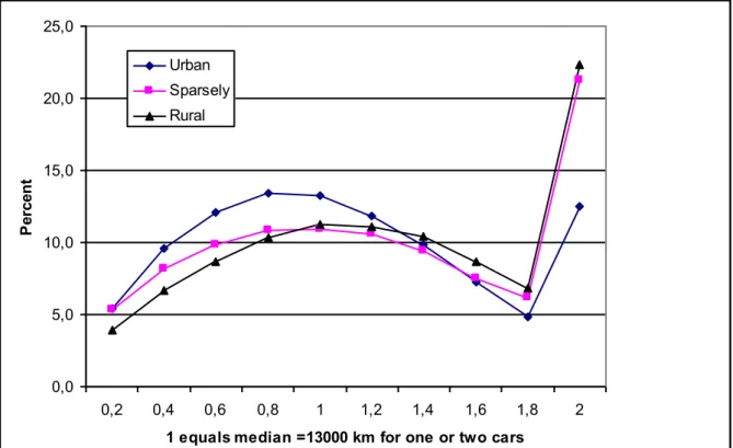
In Figure 2 the distribution of the car use for individuals owning one or two cars is presented. The number 1 represents the median of summed car use that is 13,000 kilometres. We have chosen not to give the whole scale of driving distance so the last point represents the total frequency in the tail of larger car use numbers.
By and large, the distribution of the use of cars owned by residents in rural areas is similar to that of residents in urban areas. The main difference is that that the use of cars owned by urban inhabitants which is below the median is a larger share of the population than in the whole car owner population and that car use above the median is a smaller share. For the residents in the rural areas the opposite is true. In particular, there is a relatively large share of individuals in rural areas and sparsely populated areas that use their cars really much.
Consequently the most important differences in car use between urban and the two kinds of rural areas are that more individuals own cars in rural areas and a larger share of them use their cars really much.
During the period for which the models are estimated, 1999 to 2008, the central variables developed like follows. The use of privately owned cars in the population we study increased by 6.6 percent on average. Real petrol price increased with 28 percent and average real
Taking the effect of increasing fuel efficiency over time into account, this means that an average car owner’s fuel expenditure consist the same share of the disposable income in 2008 as in 1999.
Figure 2 - Distribution of yearly car use in 2005, population median equals 13000 kilometres
3. The model and variables
The modelling framework is inspired by Dargay (2007) and specified as a dynamic panel data formulation:
ln ∑𝑛𝑓=1𝐶𝐴𝑅𝑈𝑆𝐸𝑖𝑡𝑓 = +𝛼 + 𝛾 ln ∑𝑛𝑓=1𝐶𝐴𝑅𝑈𝑆𝐸𝑖,𝑡−1,𝑓+ 𝛽1ln 𝐼𝑖𝑡+ 𝛽2ln 𝐹𝑢𝑒𝑙𝑃𝑡+ 𝛽3ln 𝐶𝑎𝑟𝑃𝑡+
𝛽4ln 𝐷𝑊𝑖𝑡+ 𝛽5𝐸𝑚𝑝𝑙𝑖𝑡+ 𝛽6𝐶𝑎𝑟2𝑖𝑡+ 𝛽7𝐶𝑎𝑟3𝑖𝑡+ 𝛽8𝐶𝑎𝑟4𝑖𝑡+ 𝛽9𝐶ℎ𝑖𝑙𝑑18𝑖𝑡+
𝜇𝑖+ 𝜖𝑖𝑡, (1)
where CARUSE represents the yearly car use calculated from odometer readings for each car f owned by an individual i in a given year t. I is individual real disposable income, FuelP is the yearly real price of petrol, CarP is the yearly real car purchase price index, DW is the distance in metres to the individual i’s workplace (takes value 1 if the individual is not working), CarX
0,0 5,0 10,0 15,0 20,0 25,0 0,2 0,4 0,6 0,8 1 1,2 1,4 1,6 1,8 2
1 equals median =13000 km for one or two cars
P er ce nt Urban Sparsely Rural
are indicators of the individual is owning X cars where X takes values 2, 3 or 4, Child18 is an indicator of one or more children over age 18 living in the home of the individual i, and 𝜇𝑖 is an individual specific effect. We use a first-difference approach for our analysis, which leads to the following model specification:
ln ∑ 𝐶𝐴𝑅𝑈𝑆𝐸𝑖𝑡𝑓− ln ∑𝑛 𝐶𝐴𝑅𝑈𝑆𝐸𝑖,𝑡−1,𝑓 𝑓=1 𝑛 𝑓=1 = 𝛾(ln ∑ 𝐶𝐴𝑅𝑈𝑆𝐸𝑖,𝑡−1,𝑓− ln ∑𝑛 𝐶𝐴𝑅𝑈𝑆𝐸𝑖,𝑡−2,𝑓 𝑓=1 𝑛 𝑓=1 ) + 𝛽1(ln 𝐼𝑖𝑡− ln 𝐼𝑖,𝑡−1) + 𝛽2(ln 𝐹𝑢𝑒𝑙𝑃𝑡− ln 𝐹𝑢𝑒𝑙𝑃𝑡−1) + 𝛽3(ln 𝐶𝑎𝑟𝑃𝑡− ln 𝐶𝑎𝑟𝑃𝑡−1) + 𝛽4(ln 𝐷𝑊𝑖𝑡− ln 𝐷𝑊𝑖,𝑡−1) + 𝛽5(𝐸𝑚𝑝𝑙𝑖𝑡− 𝐸𝑚𝑝𝑙𝑖,𝑡−1) + 𝛽6(𝐶𝑎𝑟2𝑖𝑡− 𝐶𝑎𝑟2𝑖,𝑡−1) + 𝛽7(𝐶𝑎𝑟3𝑖𝑡 − 𝐶𝑎𝑟3𝑖,𝑡−1) + 𝛽8(𝐶𝑎𝑟4𝑖𝑡− 𝐶𝑎𝑟4𝑖,𝑡−1) + 𝛽9(𝐶ℎ𝑖𝑙𝑑18𝑖𝑡− 𝐶ℎ𝑖𝑙𝑑18𝑖,𝑡−1) + 𝜖𝑖𝑡− 𝜖𝑖,𝑡−1. (2) Importantly when modelling the car use as a first-difference specification it is not possible to include time-invariant variables in the analysis. On the other hand, the individual-specific effect, 𝜇𝑖, is cancelled out in a first-difference specification. The functional form is a log-log specification, which implies that we can interpret the parameters of continuous variables as elasticities. Considering indicator variables, the parameter 𝛽𝑋 can easily be transformed to the percentage change of that indicator changing from zero to one by the formula: exp(𝛽𝑋) − 1. The functional form implies constant elasticity over all types of socio-economic groups, which is criticized by Dargay (2007). However, with the huge number of observations in this application we are able to split data to estimate group-specific models.
The dynamic part of the model, i.e. the long-run adaptation to a change that may take place in one period, implies that both the short-run and the long-run elasticity can be estimated.1 The short-run elasticities are simply the parameter estimates themselves whereas the long-run elasticities are estimated by adjusting with the dynamic parameter. For example, the long-run elasticity of income is given by 𝛽1
1−𝛾.
With access to this large data set we are able to analyse the small but politically important group of car users residing in rural areas close to an urban area and sparsely populated areas, which are considered to be particularly car dependent. Thus our model is estimated separately for the following 24 groups. The observations of individuals are separated in men and women. The individuals of these groups are allocated to three groups by type of geographical area of
residence: urban area, rural area close to urban area and sparsely populated area. The individual observations are furthermore grouped by disposable income quartiles.
This leads us to the issue of classification, where we want to keep the panels balanced as long as possible. Therefore we assign an individual to the same group over the complete time period. Geographical area type is defined in the first period and individuals are assigned to that region for all observation years. This classification approach thus does not take changed geographical regions into account, which on the other hand has occurred for only 13 percent of our sample. Income classification is based on the average individual disposal income over the observation years, with the quartile limits set by the income observed for all individuals in our data.
4. Estimation methods
By construction, a dynamic model specification as in equation (1) implies an endogeneity problem, where the traditional panel-data estimators are not consistent (see e.g. Cameron and Trivedi, 2005). Therefore, the lagged dependent variable has to be instrumented by valid and strong instruments. Theoretically consistent estimators for these kinds of models are
developed, and often known as Arellano-Bond models. However, we have tested a numerous different specifications of all these models and none of them satisfy the validity test of the included instruments.
Instead we use an instrument variable panel data estimator with appropriate lagged exogenous regressors as instruments. All estimations are performed by the user-written Stata command
xtivreg2 (Schaffer, 2010).
To produce consistent parameter estimates, the instruments must be strong and valid (Cameron and Trivedi, 2005). In our application, strong means that the instruments should explain a sufficient amount of the lagged dependent variable, whereas valid means that the instruments have to be uncorrelated with the error term in the specified dynamic panel data model. To test whether the instruments are strong and valid we rely on the tests automatically reported by Stata when using xtivreg2.
The problem of weak instruments causing bias in two-stage IV estimation is diminishing in the sample size (see e.g. Murray, 2006). With the sample sizes as large as in our application, even fairly low R2-values of our instruments will therefore not be a relevant problem.
Our instrumental variables are considered as valid since lagged explanatory variables do not affect the error term in time t. We choose those variables that are mostly correlated with the lagged dependent variable and avoid problems of weak instruments by not using too many instruments. The instruments we use are first-lagged versions of income, Child over 18 and employment. The first-stage regression of the instrumental variable-method is estimation of the model: ln ∑𝑛𝑓=1𝐶𝐴𝑅𝑈𝑆𝐸𝑖,𝑡−1,𝑓− ln ∑𝑛𝑓=1𝐶𝐴𝑅𝑈𝑆𝐸𝑖,𝑡−2,𝑓 = 𝜃1(ln 𝐼𝑖,𝑡− ln 𝐼𝑖,𝑡−1) + 𝜃2(ln 𝐹𝑢𝑒𝑙𝑃𝑡− ln 𝐹𝑢𝑒𝑙𝑃𝑡−1) + 𝜃3(ln 𝐶𝑎𝑟𝑃𝑡− ln 𝐶𝑎𝑟𝑃𝑡−1) + 𝜃4(ln 𝐷𝑊𝑖,𝑡− ln 𝐷𝑊𝑖,𝑡−1) + 𝜃5(𝐸𝑚𝑝𝑙𝑖,𝑡− 𝐸𝑚𝑝𝑙𝑖,𝑡−1) + 𝜃6(𝐶𝑎𝑟2𝑖,𝑡− 𝐶𝑎𝑟2𝑖,𝑡−1) + 𝜃7(𝐶𝑎𝑟3𝑖,𝑡− 𝐶𝑎𝑟3𝑖,𝑡−1) + 𝜃8(𝐶𝑎𝑟4𝑖,𝑡− 𝐶𝑎𝑟4𝑖,𝑡−1) + 𝜃9(𝐶ℎ𝑖𝑙𝑑18𝑖,𝑡− 𝐶ℎ𝑖𝑙𝑑18𝑖,𝑡−1) + 𝜃10(ln 𝐼𝑖,𝑡−1 - ln 𝐼𝑖,𝑡−2) + 𝜃11(𝐸𝑚𝑝𝑙𝑖,𝑡−1− 𝐸𝑚𝑝𝑙𝑖,𝑡−2) + 𝜃12(𝐶ℎ𝑖𝑙𝑑18𝑖,𝑡−1− 𝐶ℎ𝑖𝑙𝑑18𝑖,𝑡−2) + 𝜀𝑖,𝑡−1− 𝜀𝑖,𝑡−2,
where the predicted values of the dependent variable
ln ∑𝑛𝑓=1𝐶𝐴𝑅𝑈𝑆𝐸𝑖,𝑡−1,𝑓− ln ∑𝑛𝑓=1𝐶𝐴𝑅𝑈𝑆𝐸𝑖,𝑡−2,𝑓 are used in the estimated equation (2) above. Instrumental variables are (ln 𝐼𝑖,𝑡−1 – ln 𝐼𝑖,𝑡−2), (𝐸𝑚𝑝𝑙𝑖,𝑡−1− 𝐸𝑚𝑝𝑙𝑖,𝑡−2) and
(𝐶ℎ𝑖𝑙𝑑18𝑖,𝑡−1− 𝐶ℎ𝑖𝑙𝑑18𝑖,𝑡−2).
Finally, we need to adjust the standard errors for the fact that only yearly observations of fuel price and car purchase price index are available for the analysis. Even if we would have access to more detailed price data it cannot be used to map the car use since the latter is observed on a yearly basis. For the adjustment of the standard error we use the cluster option in Stata.
5. Results
In Table 3 and 4, the estimated parameters and diagnostics for all 24 sample specifications of the dynamic model are presented. A few of the models are a bit problematic regarding the results, which mainly holds for high-income groups in sparsely populated areas where the number of observations is considerably low.
Table 3 - Estimation results for instrument variable first-differences panel data models – men
Sparsely populated areas Rural areas close to urban areas Urban areas
Quartile 1 Quartile 2 Quartile 3 Quartile 4 Quartile 1 Quartile 2 Quartile 3 Quartile 4 Quartile 1 Quartile 2 Quartile 3 Quartile 4
Lagged Car Use *0.623 0.230 0.192 0.498 ***0.294 ***0.494 ***0.510 ***0.551 ***0.432 ***0.493 ***0.612 ***0.689
Disposable Income **0.028 **0.033 **0.025 *0.037 *0.008 ***0.024 ***0.032 **0.025 ***0.009 ***0.033 ***0.038 ***0.019
Petrol Price ***-0.344 ***-0.288 *-0.211 -0.030 ***-0.292 -0.166 *-0.214 -0.124 ***-0.396 **-0.295 *-0.210 -0.082
Car Purchase Price Index ***0.423 0.191 -0.007 *-0.353 **0.347 -0.148 -0.134 -0.347 *0.281 -0.040 -0.188 -0.412
Distance to Work -0.002 -0.001 *0.002 -0.001 0.000 **0.001 *0.001 *0.001 *0.001 ***0.001 ***0.001 **0.001
Children over 18 0.046 ***0.031 0.010 ***0.067 0.013 0.009 ***0.012 ***0.011 0.001 ***0.008 ***0.012 ***0.010
Employed 0.019 0.010 **-0.026 0.053 ***0.031 ***0.014 0.010 0.011 **0.014 0.005 ***0.007 **0.009
Two number of Cars ***0.350 ***0.327 ***0.358 ***0.409 ***0.369 ***0.396 ***0.426 ***0.488 ***0.517 ***0.502 ***0.515 ***0.580
Three number of Cars ***0.578 ***0.525 ***0.593 ***0.693 ***0.638 ***0.686 ***0.698 ***0.794 ***0.853 ***0.831 ***0.845 ***0.955
Four number of Cars ***0.747 ***0.675 ***0.837 ***0.841 ***0.830 ***0.897 ***0.923 ***1.027 ***1.145 ***1.125 ***1.129 ***1.267
Number of observations 58143 47004 34880 15630 457243 468555 613675 408163 910993 1303876 1675163 1703150
Root mean square error 0.78 0.66 0.62 0.68 0.65 0.75 0.72 0.68 0.71 0.70 0.71 0.68
Test of valid instruments (p-value) 0.68 0.90 0.84 0.52 0.66 0.48 0.82 0.01 0.09 0.81 0.01 0.01
Test of weak instruments (F-test
statistic) 12.83 14.64 11.66 4.23 122.54 207.52 163.24 51.75 170.76 398.98 392.05 107.88
Logarithmic car use is dependent variable.
Continuous variables are given in their natural logarithmic form.
*** indicates significant at 1 percent level, ** at 5 percent and * at 10 percent. The estimations include intercept, which are omitted here.
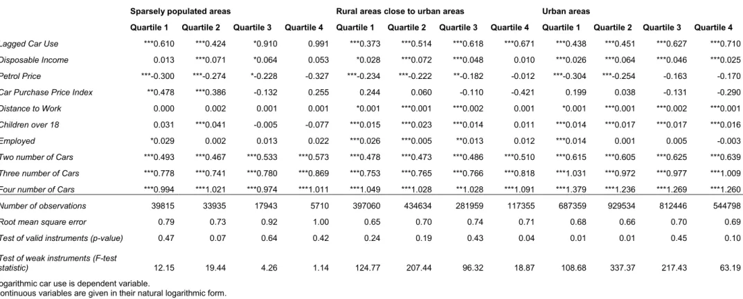
Table 4 - Estimation results for instrument variable first-differences panel data models – women
Sparsely populated areas Rural areas close to urban areas Urban areas
Quartile 1 Quartile 2 Quartile 3 Quartile 4 Quartile 1 Quartile 2 Quartile 3 Quartile 4 Quartile 1 Quartile 2 Quartile 3 Quartile 4
Lagged Car Use ***0.610 ***0.424 *0.910 0.991 ***0.373 ***0.514 ***0.618 ***0.671 ***0.438 ***0.451 ***0.627 ***0.710
Disposable Income 0.013 ***0.071 *0.064 0.053 *0.028 ***0.072 ***0.048 0.010 ***0.026 ***0.064 ***0.046 ***0.025
Petrol Price ***-0.300 ***-0.274 *-0.228 -0.327 ***-0.234 ***-0.222 **-0.182 -0.012 ***-0.304 ***-0.254 -0.163 -0.170
Car Purchase Price Index **0.478 ***0.386 -0.132 0.255 0.244 0.060 -0.110 -0.421 0.199 0.038 -0.131 -0.290
Distance to Work 0.000 0.002 0.001 0.001 *0.001 ***0.001 ***0.002 0.001 *0.001 ***0.001 ***0.002 ***0.001
Children over 18 0.031 ***0.041 -0.005 -0.077 ***0.015 ***0.023 ***0.014 0.011 ***0.014 ***0.017 ***0.017 ***0.016
Employed *0.029 0.002 0.013 0.022 ***0.026 ***0.005 **0.013 0.012 ***0.014 0.001 0.005 -0.003
Two number of Cars ***0.493 ***0.467 ***0.533 ***0.573 ***0.478 ***0.473 ***0.486 ***0.510 ***0.615 ***0.605 ***0.625 ***0.639
Three number of Cars ***0.778 ***0.741 ***0.780 ***0.869 ***0.753 ***0.765 ***0.766 ***0.818 ***1.031 ***0.972 ***0.977 ***1.009
Four number of Cars ***0.994 ***1.021 ***0.974 ***1.011 ***1.049 ***1.028 **1.028 ***1.091 ***1.379 ***1.236 ***1.269 ***1.260
Number of observations 39815 33935 17943 5710 397060 434634 281959 117355 687359 929534 812446 544798
Root mean square error 0.79 0.73 0.92 1.00 0.65 0.70 0.74 0.71 0.68 0.66 0.70 0.69
Test of valid instruments (p-value) 0.47 0.07 0.64 0.42 0.24 0.19 0.43 0.04 0.01 0.01 0.45 0.10
Test of weak instruments (F-test
statistic) 12.15 19.44 4.26 1.14 124.77 207.44 96.32 18.87 108.68 337.37 217.43 63.19
Logarithmic car use is dependent variable.
Continuous variables are given in their natural logarithmic form.
*** indicates significant at 1 percent level, ** at 5 percent and * at 10 percent. The estimations include intercept, which are omitted here.
At first, the coefficient for car use the previous year, or the inertia coefficient, is between 0.4 and 0.7 in most of our models. This implies that long-run elasticities are between 1.67 and 3.33 times higher than the short-run elasticities. Adaptation to
changed conditions is thus substantially larger in the long run than in the short run. With higher inertia adaptation will take longer time also. In the first case it will take 3 years for more than 90 percent of the adaption to take place and in the second it will take 7 years. The inertia coefficient tends to increase with income, especially for rural areas close to an urban area and urban areas. This means that the difference between short-run and long-run effects increases with income, i.e. adaptation in the long-run is relatively easier for high-income individuals.
With a few exceptions, the diagnostic tests suggest our model specification to be adequate. Specifically, there is evidence for our instrumental variables to be strong enough and also no clear evidence of non-valid instruments.
Before moving on and discuss the result of our income and fuel-price variables, we briefly present the result of the other covariates. Employed, distance to work and children over 18 are mostly positive and statistically significant. However, the size of the effects is fairly small, for example employed individuals drive their cars between 1 and 3 percent more than non-employed individuals.
The indicator variables for number of cars follow a plausible positive but diminishing trend. Noticeable is that the marginal effect of owning more cars is largest in urban areas. A possible explanation is that individuals in urban areas only own more cars if they really utilize them by driving, since the cost of and accessibility to parking lots are generally higher in urban areas compared to rural areas.
The car purchase price index shows mixed results. Most of the few statistically significant results are positive, which is a contradiction to economic theory regarding how price variables influence demanded quantity. However, the purchase price index is a mixture of new and old cars and we are a bit suspicious to the quality and relevance of this variable to our models.
Now turning to the fuel price and income effects, which we will discuss regarding short- and long-run effects as well as group differences. For convenience, these elasticities are summarized in Tables 5-8.
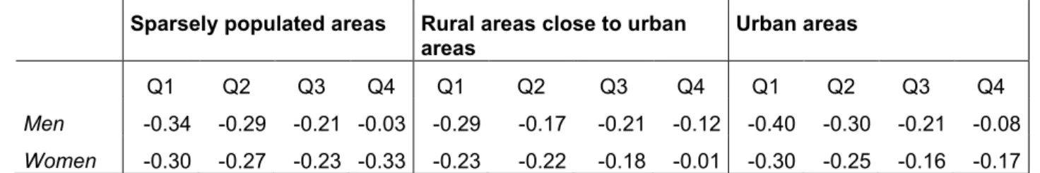
Table 5 - Short-run fuel-price elasticities of car use
Table 6 - Long-run fuel-price elasticities of car use
The fuel price elasticity is negative and non-elastic in the short run for all models, most of them in the interval -0.2 to -0.4. This means relatively low fuel price sensitivity in the short run, which correspond to the expected pattern since individuals in the short run have problems to adjust their car driving and that fuel expenditure is a small share of individuals’ total expenditure (see e.g. Vagland and Pyddoke, 2006; and Gray,
Farrington, Shaw, Martin and Roberts, 2001). Also, in the long run the elasticities are more elastic but still inelastic since all relevant estimates are below one in absolute terms. Long-run elasticities generally are between -0.3 and -0.6.
Our results correspond fairly well with the literature with a tendency towards more elastic fuel-price effects. In a previous study of Sweden, Jansson and Wall (1994) found a short-run elasticity of -0.2 and a long-run elasticity of -0.3. Dargay’s (2007) results imply a short-run elasticity of -0.18. In the surveys of Graham and Glaister (2002) and Jong and Gunn (2001) average values from a large number of studies of car use elasticities with respect to fuel price are given as: short run -0.16 and long run -0.26. A further strength of our study is that we can analyse the fuel-price elasticities
separately for groups classified by income, gender and geographical region. Here, we can observe that the fuel-price sensitivity decreases with income, which most likely is connected with a less binding budget constraint when the income is high. Furthermore, rural areas close to urban areas have the most inelastic fuel-price elasticities, especially
Sparsely populated areas Rural areas close to urban
areas Urban areas
Q1 Q2 Q3 Q4 Q1 Q2 Q3 Q4 Q1 Q2 Q3 Q4
Men -0.34 -0.29 -0.21 -0.03 -0.29 -0.17 -0.21 -0.12 -0.40 -0.30 -0.21 -0.08
Women -0.30 -0.27 -0.23 -0.33 -0.23 -0.22 -0.18 -0.01 -0.30 -0.25 -0.16 -0.17
Sparsely populated areas Rural areas close to urban areas
Urban areas
Q1 Q2 Q3 Q4 Q1 Q2 Q3 Q4 Q1 Q2 Q3 Q4
Men -0.91 -0.37 -0.26 -0.06 -0.41 -0.33 -0.44 -0.28 -0.70 -0.58 -0.54 -0.26
sparsely populated areas, the fuel-price elasticities seem to be the same as for urban areas, also when we consider the low-income quantiles. This corresponds to the fact that people living in rural areas close to an urban area are most dependent on their car and also, which can be seen from Figure 2, this group is the one with the highest average car use. Finally, when comparing men and women, there is a weak tendency of more
inelastic fuel price elasticity for women in the short run.
Turning to the income elasticities, summarized in Tables 7 and 8, we can see that they are, as expected, positive but in general fairly low with estimates between 0.01 and 0.07 in the short run and between 0.2 and 0.15 in the long run. These estimates are all clearly lower than the long-run elasticity of 1.02 for a similar specification in a British study (Dargay, 2007). The household dimension where we have used purely individual data may be a source for this difference. On the other hand, our small income effects are consistent with the change of total car driving distances on the aggregated level in an industrial country as Sweden with a high level of car saturation. As an example, statistics from Swedish Transport Analysis shows that total private car driving in Sweden was 43.7 billion kilometres in 2011 compared to 43.5 billion kilometres in 2002. Despite a real GDP-increase of about 24 percent during these years, the increase in car driving was only marginal. Furthermore, another possibly important reason is that we do not model car ownership, which may be much more dependent on income and when you already own a given number of cars, the driving distance is not strongly dependent on income. In other words, the estimated income elasticity holds for the income effect on driving the existing number of owned cars.
The income elasticities differ a bit across our different estimation groups. Income elasticity is highest for the two middle income quartiles, especially for women this effect is at present. Theoretically, we would expect a decrease in elasticity when income increases. There is indeed such tendency if we are excluding the first income quartile. It has been noted in previous studies (Pyddoke, 2009) that the income variable collected from administrative registers by default do not include unregistered incomes, which may be relatively most important when analysing low-income groups.
Table 7 - Short-run income elasticities of car use
Table 8 - Long-run income elasticities of car use
The income elasticity is higher for women than for men. The reason may be that women are generally driving less than men. Finally, there are no clear signs of different income elasticities with respect to urban, rural and sparsely populated areas.
6. Conclusions
The main objective of this paper has been to assess how low income car users living in rural areas close to an urban area and sparsely populated areas adapt their car use to fuel-price and income changes. We estimate a dynamic panel data specification based on individual register data. Endogeneity problem of the dynamic part is handled through the use of lagged regressors as instrumental variables. The huge data set of all Swedish private car owners observed from 1999 to 2008 implies the opportunity of analysing different groups with respect to gender, income and geographical region separately. Generally we indeed find some geographical differences in the sensitivity to changes in disposable income and fuel price.
The estimated fuel-price elasticities are in the short run about -0.22 and about -0.44 in the long run. As expected car fuel is a highly inelastic good, which emphasises
individuals’ cost of adjusting their car driving. Furthermore, these estimates are close to other estimates in the literature with a certain tendency for our estimates to be more elastic. One reason for a slightly more elastic price elasticity compared to the relevant
Sparsely populated areas Rural areas close to urban
areas Urban areas
Q1 Q2 Q3 Q4 Q1 Q2 Q3 Q4 Q1 Q2 Q3 Q4
Men 0.03 0.03 0.03 0.04 0.01 0.02 0.03 0.03 0.01 0.03 0.04 0.02
Women 0.01 0.07 0.06 0.05 0.03 0.07 0.05 0.01 0.03 0.06 0.05 0.03
Sparsely populated areas Rural areas close to urban areas
Urban areas
Q1 Q2 Q3 Q4 Q1 Q2 Q3 Q4 Q1 Q2 Q3 Q4
Men 0.07 0.04 0.03 0.07 0.01 0.05 0.06 0.05 0.02 0.07 0.10 0.06
newest cars and thus the exclusion of those cars from our sample. The owners of new cars most likely have higher incomes than the average car owner and are therefore also less sensitive to price changes of fuel.
There are however interesting differences across groups. The fuel-price elasticity decreases with income, which holds for both men and women as well as for all geographical regions. The highest price sensitivity is found in rural areas close to an urban area, which probably is connected with the fact that individuals in this particular geographical area type have the highest car driving average. Interestingly, this effect is most clear for the lower income groups of quartile 1 and 2. On the other hand, there is no particular difference in fuel-price sensitivity across individuals living in sparsely populated areas and urban areas. In addition, when comparing men and women, there is a weak tendency of lower fuel-price sensitivity for women in the short run.
The estimated income elasticities are fairly low and tend to decrease with increasing disposable income. This may indicate that there is some saturation in car use occurring when disposable income increases. The estimates for income elasticities appear to be reasonable compared to aggregated car driving measures in Sweden during this time period. Car saturation and the fact that we do not model car ownership may be explanations to this finding.
The other covariates are mostly statistically significant with the anticipated signs. However, distance to work, employment and children above 18 have all only marginal effects on car driving.
The effect of lagged car use, inertia, is around 0.5 which is larger than the estimated effect for households in the UK. This implies that it takes longer time for Swedish car users to fully adapt to changes in costs and income, than in the UK.
Combining these observations we may formulate the following conclusions about low income car users in rural areas. This group owns cars to a lesser degree than those with higher incomes in rural areas but more than the corresponding inhabitants in urban areas. It appears that low income earners’ car use is less fuel-price elastic in rural areas close to an urban area but not in sparsely populated areas compared to urban areas. The policy implications of, for example, increasing petrol taxes are that households will initially mostly absorb price increases by not increasing other forms of consumption. In a longer perspective increased petrol prices is likely to impact on the choice of car type.
We may also conclude that in a majority of the population there is only a weak preference for increasing car use when disposable income increases.
The car use patterns for individuals in sparsely populated areas differ a bit from other rural areas, where the latter seems to be more car dependent than the former. Therefore, in contradiction to popular beliefs, policies specially directed at subsidising the car use of inhabitants in sparsely populated areas in general, do not seem to be called for. The distributional consequences of increased petrol prices will thus be fairly even among car owners in different area types but will hurt low income car owners more as they frequently use a larger share of their disposable income for fuel expenditures. Any remedies against increases in fuel prices motivated by distributional concerns should therefore target income rather than where people live.
This paper should be seen as a first step in the analysis of socioeconomic and
geographical differences in Swedish car use. As we have a uniquely rich data set this opens a potential for further detailed analysis of car use in different social groups as well as geographical areas. In this paper we have begun this process.
The most interesting development that we foresee is to connect individuals in the same households. Although we cannot map all households using Swedish registers, we may connect individuals to households in a way that allow for a more accurate mapping of the income and cars that individuals can utilize.
There is also a selection issue in the sense that some individuals may seek to acquire the right to use a car provided by their employer. This may be particularly attractive for self-employed individuals. If the individuals that use their cars the most get cars from their employers they do not appear in our data set. This may also create a bias. A possible further extension to our models could be such selection models.
Finally, estimate precision of the fuel-price elasticity may be increased if we, by access to car-specific data, can use fuel efficiency to calculate individual-specific fuel cost per driving kilometre.
References
Bjørner, Thomas Bue, 1999, Demand for Car Ownership and Car Use in Denmark: A Micro Econometric Model, International Journal of Transport Economics, Vol. 26: 3, pp. 377-95.
Cameron, A. Colin and Trivedi, Pravin K., 2005, Microeconometrics: Methods and Applications, New York: Cambridge University Press.
Dargay, Joyce, 2007, The effect of prices and income on car travel in the UK,
Transportation Research Part A 41,949-960.
Dargay, Joyce and Hanly, Mark, 2004, Land use and mobility, Paper presented at World Conference on Transport Research.
Dargay, Joyce and Hanly, Mark, 2007, Volatility of car ownership, commuting mode and time in the UK, Transportation research Part A 41, 934-948.
Dargay, J. and Vythoulkas, P., 1999, Estimation of dynamic car ownership model: a pseudo-panel approach. Journal of Transport Economics and Policy 33 (3), 283–302. Graham, D. and Glaister, S., 2002, Review of income and price elasticities of demand for road traffic, Center for Transport Studies, Imperial College of Science London. Gray, D.; Farrington, J.; Shaw, J.; Martin, S.; Roberts, D., 2001, Car dependence in rural Scotland: Transport policy, devolution and the impact of the fuel duty escalator,
Journal of Rural Studies 17 (1), 113-125.
Jansson J.-O. and Wall R., 1994, Bensinskatteförändringars effekter, Rapport till Expertgruppen för Studier i offentlig ekonomi.
Jong, G.C. de (1990), An indirect utility model of car ownership and private car use,
European Economic Review 34, 971-985.
Jong, G.C. de and Gunn H., 2001, Recent evidence on car cost and time elasticities of travel demand in Europe, Journal of Transport Economics and Policy 35, 137-160. Krantz, L.-G., 1999, Rörlighetens mångfald och förändring, Befolkningens dagliga resande I Sverige 1978 och 1996, Meddelanden från Göteborgs universitets geografiska institutioner, Serie B, Nr 95, Handelshögskolan vid Göteborgs universitet.
Matstoms, P., 2002, Modeller och prognoser för arealt bilinnehav i Sverige. VTI-rapport 476.
Murray, M.P., 2006, Avoiding Invalid Instruments and Coping with Weak Instruments,
Journal of Economic Perspectives 20 (4), 111-132.
Pyddoke, R., 2009, Empirical analyses of car ownership and car use in Sweden. VTI-Rapport 653.
Rouwendal, J. och de Vries, F., 1999, Short term reactions to changes in fuel prices - a panel data analysis, International Journal of Transport Economics 3 (26), 331-350. Riks-RVU/RES 1994-2001.
Schaffer, M.E., 2010, xtivreg2: Stata module to perform extended IV/2SLS, GMM and AC/HAC, LIML and k-class regression for panel data models.
http://ideas.repec.org/c/boc/bocode/s456501.html. SIKA 2007, RES 2005-2006.
Stock, J. H. and Yogo, M., 2004, Testing for Weak Instruments in Linear IV
Regression. Identification and Inference for Econometric Models: Essays in Honor of Thomas Rothenberg, 2005.
Vagland, Å. and Pyddoke, R., 2006, Hur hushållen anpassar sig till ändrade kostnader för bilinnehav och bilanvändning? VTI-rapport 545.