The Phillips Curve and the Global Financial Crisis : A study on the Nordic countries from 1999 to 2016

The Phillips Curve and the

Global Financial Crisis

BACHELOR THESIS WITHIN: Economics NUMBER OF CREDITS: 15 ECTS

PROGRAMME OF STUDY: International Economics AUTHOR: Henri Lepa 960107 Linh Dieu Pham 961128 SUPERVISORS: Emma Lappi

Michael Olsson

Bachelor Thesis in Economic

Title: The Phillips Curve and the Global Financial Crisis Authors: Henri Lepa and Linh Dieu Pham

Tutor: Emma Lappi and Michael Olsson Date: 2018-05-21

Key terms: Unemployment, inflation, Phillips Curve, economic crisis, Global Financial Crisis, Nordic countries.

Abstract

This paper examines the effects of the Global Financial Crisis on the relationship between unemployment and inflation rate through the Phillips Curve in five Nordic countries: Denmark, Finland, Iceland, Norway and Sweden, from 1999 to 2016. The Nordic countries are quite unique in the world, as they are all economically and culturally connected to each other, which allows us to analyse how the crisis affected them differently. The foundation of our research is the Phillips Curve, which shows an inverse relationship between unemployment and inflation. By using the two-way fixed effects model, we have investigated whether the Phillips Curve and the relationship still holds during the time of the crisis for the Nordic countries. The results have shown that the relationship has changed during the crisis period, which might be due to the unemployment shock and the low targeted inflation rate.

Table of Contents

1.

Introduction ... 1

1.1 Purpose ... 2

2.

The Global Financial Crisis ... 4

2.1 The Global Financial Crisis in the Nordic countries ... 5

2.1.1 Denmark ... 7 2.1.2 Finland ... 7 2.1.3 Iceland ... 8 2.1.4 Norway ... 8 2.1.5 Sweden ... 8

3.

Literature ... 10

4.

Methodology ... 14

5.

Empirical results ... 20

5.1 Two-way fixed effect ... 20

5.2 OLS ... 23

6.

Discussion ... 25

7.

Conclusion ... 27

8.

Reference list ... 28

1. Introduction

According to Hayo (1998), inflation shows how stable prices in a certain country are. Another economic aspect that economists are interested in is unemployment, which does not only affect individuals but also the economy as a whole. How does inflation affect unemployment and vice versa? It has been investigated that there is a relationship between unemployment and inflation in the short run, which has been studied by William Phillips in the United Kingdom from 1861 to 1957. Phillips introduced the Phillips Curve (PC), which shows the inverse relationship between inflation and unemployment. The Phillips Curve shows that a higher inflation rate corresponds to a lower unemployment level, hence, there is a trade-off between the two factors (Phillips, 1958). The trade-off was believed to be something that the policymakers could exploit and benefit from, which would help the economy (Cashell, 2014). However, this theory has been questioned after the Great Inflation in the 1970, when both high unemployment and high inflation were recorded.

There were three major crises between 1991 and 2012: the Nordic Financial crisis during the early 1990; the Internet (IT) bubble during 1997-2003, and the Global Financial Crisis, which was also known as the Great Recession, occurred 2007-2008. On the world’s scale, during the IT bubble, gross domestic product (GDP) growth experienced a slight decrease with a dip to 1.923% from 4.396%. However, during the Global Financial Crisis experienced a fall from 4.255% (2007) to -1.738% (2008), the lowest it had been since World War II for the world (Data World Bank, 2018). Thus, we are going to focus on the Great Recession to have a further look into the effects on the relationship between inflation and unemployment rate. The Nordic countries consist of Denmark, Finland, Iceland, Norway and Sweden; and the Faroe Islands, including Åland and Greenland, which are under the territory of Finland and Denmark, respectively. Unlike the other countries in the group, Finland belongs to the European Monetary Union and uses the Euro as their official currency. Despite this, all these countries have a strong economic bond and have an important role regarding trade. This is mainly due to the close distance between the countries, which is indicated by the gravity model (Isard, 1954). A noticeable example for this is Sweden, which mostly trades with Norway, Finland, and Denmark, where 27% of the country exported goods go to (Statistics Sweden, 2018).

As the Nordic region are considered small open economies in the terms of the world, they are dependent on international developments (Gylfason, Holmström, Korkman, Söderström & Vihriälä, 2010). The Nordic countries are known for the high living standard, but most known for the economic opportunity and equality in the region. The major attributes of the Nordics include large welfare state, high rate of investment in human capital and high labour market participation. Risk sharing and a safety net to help workers to cope with risks and changes are key features of the Nordic Model. It also has the “bumblebee” feature; having high taxes with large welfare system yet still maintaining its sustainability (Andersen, 2007). The model’s goal is to maintain a stable economic and social climate, especially during the time of globalization and demographic change of an aging population.

The Global Financial Crisis had a large effect on the economy for many countries, such as the United States (US), and the Nordic countries were not an exception. They are relatively small economies that rely mainly on exports, so they were heavily affected by the crisis (Lin, Edvinsson, Chen & Beding, 2014). Aside from the direct effects that could be seen from the stock markets, the impact of economic crisis also had severe effects on spending, output, and employment. Thus, the relationship between unemployment and inflation would also be affected, and to estimate the effect, the original Phillips Curve will be used.

1.1 Purpose

The purpose of this study is to investigate how the crisis affects the relationship between unemployment and inflation during chosen the period from 1999 to 2016 for the Nordic countries. Hence, main research question of this study: What is the effect of the Global Financial

Crisis on the relationship between inflation and unemployment rate in the Nordic countries? There are

several reasons why we have chosen to have this research question. Previous studies have mentioned the effect of the financial crisis on the relationship between unemployment and inflation in the United States and the European Union (EU) but not for the Nordics nations, and this is the main contribution of the thesis. Our choice of grouping the Nordic countries together is due to the Nordic Model, which capture the combination of free market capitalism and social benefits. Therefore, it would be interesting to see how the crisis affected the group and contribute to further understanding the differences in the impact of economic crisis. The study will investigate into whether it is possible to observe the full effect of the crisis as a group despite different central banks control in each country. We also want to see

whether using the Phillips Curve for future monetary planning would be sufficient, especially during the time of crisis. It is important to also see how the crisis can affect two of economics’ most important indicators, which could help on further understanding the magnitude and aftermath of the event. This will also be discussed in connection to different elements that could have affected our results.

2. The Global Financial Crisis

The Global Financial Crisis occurred in December 2007 and was caused by the subprime mortgage originated in the US. The housing bubble burst as a result of risky loans and has led to the world’s worst economic crisis after the Great Depression. However, this was not the case for every country, China and India grew substantially during this period. It has been argued that the crisis has its roots in global imbalances, where the emerging economies, such as, China, had a current account surplus, at the expense of the US current account deficits (Liang, 2012).

The World’s GDP growth per capita started to drop from 2.98% in 2007 to a new low of -2.93% in 2010 (The World Bank, 2018). During the crisis, trading has also been decreased and the industrial production had slowed down, namely 31% in Japan, 26% in Korea, and 15% in Brazil (Evans-Pritchard, 2009). This was shown by a decrease in imports, from 19.356 trillion USD in 2008 to 15.513 trillion USD in 2009; as well as for export, from 19.681 trillion USD in 2008 to 15.856 trillion USD (Data World Bank, 2018).

In Europe, not only was the economic activity affected but also the real output which influenced the long-term growth outlook. Europe was mainly affected by the financial and banking system itself and the decrease in its value, which was considered even larger when comparing to the US. Furthermore, as the lending requirements got stricter and the households experienced a drop in their wealth, the demand for manufacturing goods decreased which had an adverse shock on the financial markets. Moreover, since the demand for manufactured goods decreased, the exports and imports fell, since the industry is dependent on trade (European Commission, 2009).

From the world perspective, there has been an increase in the unemployment rate, from 5.81% in 2008 to 6.98% in 2009, and inflation from 5.11% in 2007 to 8.95% in 2008, respectively (Data World Bank, 2018). This resulted in millions of jobs lost, affecting the welfare as well as living standards of people around the world. Taking into account of the relationship between unemployment and inflation, researches have been done on the US economy in order to see if the global crisis had changed the Phillips Curve. The answer to this is no. Laseen & Taheri Sanjani (2016) have shown that the relationship did not change during this time. The same result has also been shown by Blanchard (2016), which has proven that the Phillips Curve in the US is still the same compared to the 1960. He also found that

the slope of the curve has been declining but it was not due to the crisis. The decline has already started since the 1980, and the actual states of the US’ Phillips Curve has remained quite stable since.

This was not the case for the Euro currency area. Researches have been conducted on Eurozone countries with different conclusions being drawn. Anderton and Bonthuis (2015) shown the flattening of the PC, while Bulligan and Viviano (2017) shown that the PC is becoming steeper. The study had shown that different countries had shown to have different results. Germany experienced steeper PC compares to other countries, but became flatter during the crisis, while Italy, France, and Spain have a steeper PC towards unemployment (Bulligan & Viviano, 2017). The flatter Phillips Curve shown that the trade-off between unemployment and inflation no longer holds true.

2.1 The Global Financial Crisis in the Nordic countries

Firstly, we will have a look at the unemployment rate. All the countries have quite different unemployment levels prior to the recession, with Sweden and Finland experienced high fluctuations throughout the period from 1999 to 2006. Finland has the highest unemployment out of all the countries but starts to have a sharp decrease from 2004 until the crisis starts. Sweden also has a major decrease from 1999 to 2001, but in 2002, it starts to pick up the increasing trend again.

It can be seen that an increase started in all of these countries in 2008, especially in Iceland and Denmark, which has the lowest rate prior to the crisis. However, the high unemployment rate in Iceland quickly dropped at the end of the crisis, from its peak at 7.6% in 2010 to 7% in 2011, and keeping the trend onwards, whereas in Denmark, only a slight decrease can be seen. Even though prior to the crisis, Finland and Sweden experienced major changes, they seem to be relatively calm during the crisis, with only a slight increase.

After 2011, most of the countries seem to begin decreasing, aside from Finland and Norway, both started to increase from 2012. However, the only country that has a relatively stable unemployment rate during the entire period is Norway, remaining the rate between two percent and four percent.

Figure 1. Unemployment rate in Nordic countries 1999-2016 Source: World Bank

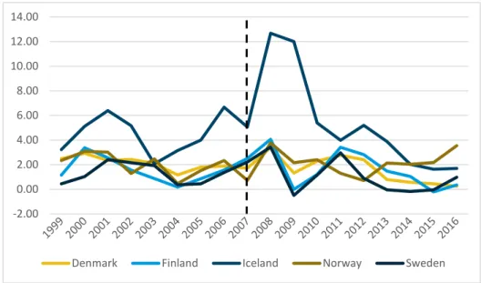
When comparing figure 1 and figure 2, there is a lag between the inflation and unemployment, inflation took on the effect of the crisis right after it started, while it took unemployment a year to start increasing. However, this is explained by the Phillips Curve, where lower inflation would mean higher unemployment rate for most of the countries, aside from Iceland.

Most of the Nordic countries, except for Iceland, have similar trend regarding the inflation rate, keeping it around 2+/-1%, this is due to the inflation target starting in the early 1990. There was some fluctuation during the recession. At the beginning of the Global Financial Crisis, we could see that there was an increase in the inflation rate for all the countries in 2008. However, the rate immediately dropped in the next year these countries, and even to the negative inflation rate in Sweden. The rates changed again to positive in 2010 and kept declining for most of the countries, except for Norway.

Sweden and Finland were the only two countries that experienced negative inflation rate during the observed period. This negative inflation could be explained by the monetary model of endogenous growth, suggesting the negative inflation-growth effect (Gillman, Harris and Mátyás, 2004). Hence, these countries wanted to lower the inflation for a positive growth. 0.00 2.00 4.00 6.00 8.00 10.00 12.00 14.00

Figure 2. Inflation rate in Nordic countries 1999-2016 Source: World Bank

To get a better understanding of the reasoning behind the effects of the Great Recession in the Nordic countries, each country will be looked at separately.

2.1.1 Denmark

Prior to the Global Financial Crisis, the Danish economy was overheated since 2005 due to the rapidly rising housing prices, as the credit policies in Denmark were lacking strictness and were managed badly. This led to deposit deficit which was impossible to finance when the interbank money market froze (Carstensen, 2011). Although the GDP of Denmark did not decrease significantly, it experienced a large increase in the unemployment rate, as can be seen from figure 1. Luckily, for Denmark, the government had large budget surpluses and strong fiscal position, when entering the recession, which helped them to decrease the impact of the crisis. During the crisis, the government took several temporary measures, to cope with the crisis and maintain the credibility of the banks (Lin, Edvinsson, Chen & Beding, 2014).

2.1.2 Finland

Although the banking sector in Finland was well-managed, Finland experienced a higher GDP loss than other Organisation for Economic Co-operation and Development (OECD) countries (Tervanen, 2009). That can largely be because of the rapid decrease in the trade in the IT sector and to one of its larger export markets in Russia (OECD, 2010a). Moreover, as the Finnish financial market is highly internationalized, it is really sensitive to the global

-2.00 0.00 2.00 4.00 6.00 8.00 10.00 12.00 14.00

crisis. In addition to that, Finland was involved in the Icelandic banks, which meant that the crash in Iceland, affected the banks’ branches in Finland as well (Tervanen, 2009). To reduce the aftermath of the crisis, the state, for example, reduced taxes, increase welfare benefits and a large portion of the taxes were spread to the local communities (Lin, Edvinsson, Chen & Beding, 2014).

2.1.3 Iceland

Before the crisis, Iceland had achieved high growth rates and quite low unemployment, which partially was due to the boom in demand after the privatization of the banking sector in the 2000. As in the case of Denmark, prior to the crisis, the housing market was overheated. This was accompanied by high inflation and high household and corporate debts, which were mainly in the Icelandic banks (Kredittilsynet, 2009). The expansions of the Icelandic banks to abroad and relatively large foreign currency debt led to a depreciation of the Icelandic currency and the collapse of three biggest banks. This is one of the reasons why the inflation rate in Iceland was relatively higher during the crisis years compared to others. Furthermore, the country’s current account was in deficit and the risk in the local financial market was high. After the collapse of the banking sector, the government needed to stabilize their currency, reduce their deficit and lower the inflation, if only to name some of their priorities. The country also got help from IMF in order to stabilize the economy (Lin, Edvinsson, Chen & Beding, 2014).

2.1.4 Norway

Norway’s economy differs a bit from other Nordic countries, as it is a combination of free-market and government intervention and it is dependent on the oil sector (OECD, 2010b). Furthermore, the country’s financial market depends heavily on the dollar, which meant when the Lehman Brothers’ collapsed, the situation for Norwegian banks worsened (Kredittilsynet, 2009). That led to a drop in the stock market and consumption which led to a negative GDP growth. However, the unemployment rate rose relatively less than in other Nordic countries. Although Norway’s situation was not bad, they still took action and through that, managed to strengthen the banks (Lin, Edvinsson, Chen & Beding, 2014).

2.1.5 Sweden

Sweden’s high dependency on the exports to international markets was one of the reasons behind the country’s crash during the crisis in 2008, despite the fact the financial market in Sweden was highly regulated due to the crisis in the 1990 (Öberg, 2009). The government

adopted a plan to stabilize the economy. Due to a well-managed financial system, they managed to stimulate the economy by supporting the labour market and cutting the tax rates, like the corporate tax. Additionally, they created a guarantee program to support the banks. All the government’s efforts helped to decrease the scope and the length of the financial crisis in Sweden (Jochem, 2010).

3. Literature

In this section, theory of the Phillips Curve, critiques on the applicability of Phillips Curve and the New Keynesian Phillips Curve will be discussed. A brief introduction of the Okun’s Law is also provided.

3.1 Phillips Curve

W. Phillips was the first to investigate the relationship between inflation and unemployment. The research was done using the rate of change of money wage and unemployment in the UK. He concluded that there is a trade-off, an inverse relationship between unemployment and inflation, showing that the higher the unemployment rate, the lower inflation would be (Phillips, 1958). This view was believed to be stable in the early 1960, however, Friedman and Phelps have challenged this view. They stated that the trade-off is only temporary, and that the government could not keep increasing the inflation rate in order to maintain a low unemployment rate or vice versa. The relation can be expressed as follows (Blanchard, Giavazzi & Amighini, 2010):

𝜋𝑡 = (𝑧 + µ) − 𝛼𝑢𝑡 (1) where 𝜋_𝑡 is inflation, 𝑢_𝑡 is unemployment, 𝑧 is the catchall variable, 𝜇 is the mark-up, 𝛼 is a constant with the expected value to be negative. There is no expected inflation due to in Phillips’s time, the inflation rate was almost close to zero.

Another version of the Philips Curve is the augmented Phillips curve taking into consideration of the expected inflation rate developed by Phelps and Friedman.

𝜋𝑡 = 𝜋𝑡𝑒+ 𝛼(𝑢𝑡− 𝑢𝑡∗ ) + 𝜖𝑡 (2) where 𝜋 is inflation, 𝜋𝑒 _{is the expected inflation, 𝑢 is unemployment, 𝑢}∗ _{is the natural rate} of unemployment, 𝜖 is the error term and 𝛼 is a constant with the expected value to be negative.

Ireland (1999) found that inflation and unemployment are cointegrated through testing a Barro-Gordon hypothesis, which was shown by Shadman-Mehta (2001). However, neither have shown evidence of causality between inflation and unemployment. Nevertheless, the Phillips Curve says that the changes in inflation lag behind unemployment. Thus, it could be

used to forecast future inflation and be useful when country’s policy aim is to target inflation (Napolitano & Montagnoli, 2010).

There have been several studies done on the linearity of the Phillips Curve. When the Phillips Curve is linear the shocks have an equal effect on the relationship and the overall effect would be zero on average. In contrast, when the relationship is nonlinear, positive shocks have a greater effect than negative shocks on inflation, which would lead to a lower average unemployment rate if the right policies are used straight away. Thus, the convex Phillips Curve is more realistic (Laxton, Rose & Tambakis, 1999). Stiglitz (1997) states that in the existence of monopolistic competition, the firms are willing to lower their prices when the economic growth is slow, but not to increase the prices when there is a boom, leading to an excess demand.

As an opposition to the original view from Phillips, it is suggested that there should be a short run and a long run Phillips Curve, which in the long run, the curve would be vertical. Moreover, with adaptive expectation, the expected inflation rate would gradually converge to the actual inflation rate, and the unemployment would return to its natural level (Friedman, 1968) (Phelps, 1967). This view was not popular until Friedman successfully predicted the Great Inflation during the 1970. This was when many countries had experienced stagflation, a combination of slow economic growth with rising prices (Law, 2014). A country could experience both rising inflation and rising unemployment rate under stagflation, which is in contrast with what Phillips has found. An argument had been brought up by Friedman (1968) saying that once a high inflation rate has been set, unemployment would catch up, which is defined as the natural rate of unemployment. This concept has been reintroduced as Non-Accelerating Inflation Rate of Unemployment (NAIRU) in 1975 by Modigliani and Papademos. NAIRU puts forward that instead of focusing on choosing between either higher inflation or higher unemployment, policymakers should target just one, either low inflation or low unemployment (Modigliani & Papademos, 1975).

The Taylor’s Rule, a guideline that has been made for the central bank to use monetary policy to alter interest rate in order to keep the economic balance in the long run, states that instead of looking at the expected rates, actual rates should be considered. During a transition, the impact of the policy rule would be different from the expectations. Hence, focusing on the real inflation rate and employment would benefit the policymakers in a greater way, and allow

Robert (1995) first introduced the New Keynesian Phillips Curve (NKPC), which was based on the studies from Taylor (1980) and Calvo’s (1983), has put an emphasis on how important stickiness is to monetary policy. This was followed by numerous studies of others on developing a new model that is more fitting to the newly developed economy, with some of the most popular papers from Fuhrer (1997), Redebusch (2002) and Sbordone (2002). A majority of recent research papers are based on the NKPC instead of the classical because it is too simple for the modern economy, and it might not be useful enough for monetary policy evaluation (Soderstrom, Soderlind & Vredin, 2005). However, it has been pointed out that there is a degree of inflation in persistence, hence it is not suitable for policy analysis (Rudd & Whelan, 2001). This was also backed up by the arguments on the robust to weak identification on this model and the possibility of spurious correlation on the role of lagged inflation (Nason & Smith, 2008).

The Phillips Curve has gotten some critique about its applicability to different countries (Forder, 2014). Hines (1964) thought that trade-union membership would be more useful when predicting wage inflation. Kuh (1967) suggested that instead of unemployment, productivity should be used. In recent years, Roberts (2017) said that using the Phillips Curve, the Reagan Administrator made budget forecasting incorrect, which is a reason for the large increases in the money supply.

Despite the critiques, and that the Phillips Curve has been widely viewed as not applicable. Gali (2011) has stated the Phillips Curve has returned through the New Keynesian model. The paper has shown that the relationship between wage inflation and inflation in the US still hold under strong assumption of a constant natural rate of unemployment even under price stability. This argument has also been backed up by Gordon (2013) demonstrating that the Phillips Curve is alive and well, and capable of explaining the behaviour of the US’ inflation rate. Svensson (2008) from Riksbanken has also claim the use of the Phillips Curve for policy making in Sweden (Fuhrer, 2009).

3.2 Okun’s Law

As one of the focal point among economists, GDP is a measurement for the market value for all final goods and services, which shows the health and the performance of a country’s economy. According to Okun’s Law (1962), there is an inverse relationship between the unemployment rate and GDP growth, stating that a one percent rise in the natural rate of

unemployment will result in a three percent decrease in national output. Due to the increase in size of the labour force and productivity level, in order to reduce the unemployment rate, the economy must grow at a rate above its potential. The GDP decrease has been adjusted to two percent in a more recent research by Freeman (2000). The model was developed by Okun (1962):

∆𝑢𝑡 = 𝛼 − 𝛽𝑦𝑡+ 𝜀𝑡 (1) where ∆𝑢𝑡 is the change in the unemployment rate, 𝑦𝑡 is the GDP growth rate and 𝜀𝑡 is the error term, 𝛽 is the Okun’s coefficient and 𝛼 is a constant.

This negative relationship was reinforced by Barro’s research in 1995. The data was gathered from 100 countries between 1960 and 1990 and resulted in the observation that an increase of 10% point in unemployment will lead to a decrease in 0.2%-0.3% point in GDP growth. The effect of Okun’s Law is country specific, during the Great Recession, while Germany and the Netherlands experienced a weakened relationship, Denmark and Canada had a significant increase. This is due to, firstly, the labour institutions, which tend to restrict the employers to fire workers, unemployment responding less to output changes during the expansion period. In addition to that, it has been argued that during the times of recession the employers are more pessimistic, leading to a decline in employment (Cazes, Verick & Al Hussami, 2013).

The literature has shown that the relationship between unemployment and inflation, presented by the Phillips Curve is ambiguous. Taking into consideration of the crisis period; hence, the Great Recession had changed the relationship between unemployment and inflation for the Nordic countries. The hypothesis is formulated in accordance with the original research, as there is a trade-off between the unemployment and the inflation rate, but also consider the different results achieved.

4. Methodology

This section shows the data, dependent variable, independent variables and the applied model.

4.1 Data

The data is retrieved from the World Bank and OECD database. The gathered data is for the chosen period from 1999 to 2016. The reasoning behind the timeframe is that it allows us to see the effect of the crisis on the relationship from the period before and also after the crisis for a better observation. Three control variables were also added to the regression to have a better control of the effect on the relationship between inflation and unemployment.

4.2 Dependent Variable

The first dependent variable in this analysis is the inflation rate, which is also the main focus of our thesis. According to the Phillips Curve in the short run has an inverse relationship to the unemployment. The inflation rate is measured as the yearly change in consumer price index (CPI) (Data World Bank, 2018). The yearly data of the inflation rate is gathered from the World Bank database.

4.3 Independent variables

The unemployment rate is the main independent variable in this analysis and is measured on a yearly basis. According to the World Bank (2018), unemployment is defined as the percentage of the labour force that does not have work but are seeking employment. There are some differences between the countries in the definition of the labour force.1

The first control variable used in the model is GDP growth rate. According to Keynesian model, in the short run, the AS curve is upward sloping, hence there is a positive relationship between inflation and GDP growth rate (Dornbusch, Fischer & Kearney, 1995). GDP is a measurement of the market value for all final goods and service. It also indicates the

1 _{According to Statistics Norway, prior to 2006 their labour force survey (LFS) included people aged 16-74}

since 2006 it includes people aged 15-74 ("Labour Force Survey", 2018). In addition to that, until 2000 Sweden defined the labour force as people aged 16-64 and from 2001 they defined it as 15-74 ("Labour Force Surveys", 2018). All other countries – Finland, Denmark and Iceland – use the ages 15-74 to define the labour force. In

economic performance of the country. Therefore, if GDP growth is positive, it means that the economic health is well. However, if the GDP growth is negative, the country might be in a recession, which would affect trade and employment through productivity. The data is gathered annually from the World Bank database.

The second control variable is the exchange rate. As the inflation shows the changes in the price level, the exchange rate might mainly affect the price of foreign goods. Dornbusch (1986) found out in his study that the depreciation of the currency will raise the inflation rate. Also, worth noting is that in the years 1999 to 2002 Finland used Finnish Markka as their currency, but Euro was also used as currency, during the transition period, so in this analysis, the exchange rates for Euro was used throughout the time period for Finland. The exchange rate for all the currencies is gathered on yearly basis from the World Bank database and is measured in US dollar (as exchange for local currency).

The third control variable is the annual wage growth. When describing the relationship between wage and inflation, the term wage-push inflation is used. This states that, an increase in prices will be caused by the rise of the wage level, which then increases the cost of production ("Wage-push inflation", 2018). The annual data for wage is gathered from the OECD database and measured in USD, an additional year for 1998 was collected to calculate the growth for 1999, then to calculate for the annual wage growth rate, the following equation was used:

𝑊𝑎𝑔𝑒 𝑔𝑟𝑜𝑤𝑡ℎ 𝑟𝑎𝑡𝑒 = ( 𝑤𝑎𝑔𝑒_{𝑤𝑎𝑔𝑒}𝑡− 𝑤𝑎𝑔𝑒𝑡−1

𝑡−1 )100 (4)

where 𝑤𝑎𝑔𝑒𝑡 is the present wage annual rate and 𝑤𝑎𝑔𝑒𝑡−1 is the previous annual wage rate. Finally, dummy variables are added to unemployment the year from 2007, which allows us to see if the crisis have had any effects on the observed relationship. The dummy variable (Dt) used in the regression indicates the period after the crisis. Hence, the years 1999-2006

has a value of zero and the years 2007-2016 the dummy takes a value of one. The use of the dummy will allow us to see how the relationship changed after the crisis. Therefore, the unemployment is multiplied with the dummy variable to capture the effects of the crisis on the relationship between the unemployment and inflation, whether the correlation still remains unchanged.

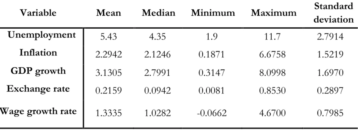
4.4 Descriptive statistics

To get an overview and the description of the independent and control variables, the descriptive statistics can be found in table 1 and 2. The thesis is focused on two periods, the first is shown in Table 1, which looks at the period before the crisis and the second period in Table 2, which captures the time during and after the crisis. The tables include the mean, median, standard deviations, maximum and minimum values for the variables used in the regressions. The standard deviation shows how much the values deviate from the mean.

Table 1 - Descriptive statistics for the period before crisis (1999-2006)

Variable Mean Median Minimum Maximum Standard deviation Unemployment _{5.43 4.35 1.9 11.7 2.7914}

Inflation _{2.2942 2.1246 0.1871 6.6758 1.5219} GDP growth _{3.1305 2.7991 0.3147 8.0998 1.6970} Exchange rate _{0.2159 0.0942 0.0081 0.8530 0.2897} Wage growth rate _{1.3335 1.0282 -0.0662 4.6700 0.7985}

Looking at Figure 1, which shows the unemployment rate in the Nordic countries, Finland already had a relatively high unemployment in the beginning of the period, driving the mean and median of the unemployment up. This could be the result of the early 2000 IT Bubble. Other countries are more stable economically which drives the mean down to a more stable value, with Iceland and Norway having relatively low unemployment rate during this period. The inflation’ mean and median do not differ much, however the maximum is quite high, the value is recorded in 2006 in Iceland. GDP growth had a high maximum from Iceland at 8.0998% in 2004, showing that before the crisis, Iceland was expanding. However, due to lower rate in other countries, especially Denmark, the mean and median was driven down. The exchange rate has also higher span of value, which can be explained by the exchange rate of the Icelandic currency, which is lower than others, this also lowers the value of the mean. During the before crisis period the exchange rates in these countries had an increasing trend overall. The wage growth rate, before the crisis, in the Nordic countries varied quite lot from -0.06 to 4.67 percent, this is mainly due to higher wage growth rates in the end of the 1990, after 2000 the wage shows a small growth, only around 1 percent.

Table 2 - Descriptive statistics for the period during and after crisis (2007-2016)

Variable Mean Median Minimum Maximum Standard deviation Unemployment _{6.034 6.5 2.2 9.4 2.0914}

Inflation _{2.3606 2.0300 -0.4945 12.6782 2.5324} GDP growth _{1.1686 1.4281 -8.2690 9.3501 3.1624} Exchange rate _{0.2372 0.1066 0.0052 0.9293 0.3203} Wage growth rate _{1.0287 1.0122 -0.4282 2.2853 0.3965}

In the period of during and after crisis, the unemployment rate shows more stable values and the maximum value is lower than that of the before crisis period. As mentioned before, Finland’s unemployment rate drives the mean value of unemployment before the crisis up. Most of the extreme values were recorded during and after the crisis, and returned to their prior levels afterwards, which affected the overall mean and median. Iceland had also experienced higher unemployment rates in the previous period, but unable to keep the unemployment low due to the harsh economic conditions during the crisis. In addition to that, the Icelandic Krona experienced a depreciation during the crisis and was impacted from their own banking crisis, which led to the collapse of its three major banks. These events led to higher inflation and the exchange rate decreased. In addition to that, the exchange rate had a peak value during the crisis, which increased the value of mean and the standard deviation in general. The inflation rate remains similar to before crisis regarding mean and median. However, negative inflation was recorded in Sweden and significantly lower than the maximum by about 13 unit in Iceland. The low minimum in GDP growth was in Finland, which was explained by the country’s poor economic policies. And the highest value was from Iceland, however this was in 2007, and the effect of the crisis did not take place until 2008. The trend for growth in all the countries were negative during the time of recession, hence the mean and median value seems to be quite low, even though all the countries had an increase shortly after 2008-2009. During and after the crisis, the wage growth rates had still higher differences between countries and between minimum and maximum values, but the span of the values were smaller, which of course can be explained by the effect the crisis had on wages and its growth rates.

4.5 Correlation matrix

In the table 3, the correlation matrix, presents a Spearman correlation coefficient, ranging between -1 and +1 (Gujarati, 2003). The highest Spearmen correlation coefficient value is 0.5902, which is between unemployment and natural logarithm of the exchange rate. In the next section both regressions, two-way fixed effects, and the OLS, were ran by removing the exchange rate from the regression to see how the exchange rate affected the result. Also, the fixed effects model was tested for autocorrelation using the Breusch-Pagan LM test, which turned out to be significant. The result of the test is presented in the Appendix.

Table 3 - Correlation Matrix

𝑖𝑖𝑡 𝑢𝑒𝑖𝑡 𝑢𝑒𝑖𝑡𝐷𝑡 𝑌𝑖𝑡 𝑤𝑖𝑡 ln (𝑒𝑖𝑡) 𝜋_𝑖𝑡 1 𝑢𝑒_𝑖𝑡 -0.3318 1 𝑢𝑒𝑖𝑡𝐷𝑡 -0.0873 0.4080 1 𝑌𝑖𝑡 -0.0690 -0.1786 -0.4216 1 𝑤_𝑖𝑡 -0.0925 -0.1352 -0.2463 0.0399 1 𝑙𝑛(𝑒_𝑖𝑡) -0.5278 0.5902 0.1375 -0.1638 -0.0481 1 4.6 Model

The model used in the analysis is based on the Phillips Curve. Due to the problem with expected inflation, we will be using a modified version of the Phillips Curve. The analysis is done by using panel data analysis and using a two-way fixed effect model. The equation for the model is as follows:

𝜋𝑖𝑡 = 𝛽0+ 𝛽1𝑢𝑒𝑖𝑡+ 𝛽2𝑢𝑒𝑖𝑡𝐷𝑡+ 𝛽3𝑌𝑖𝑡+ 𝛽4𝑙𝑛 (𝑒𝑖𝑡) + 𝛽5𝑤𝑖𝑡+ 𝛼𝑖+ 𝛿𝑡+ 𝑢𝑖𝑡 (4) where 𝜋𝑖𝑡 represents the country and t represent the year, 𝛼𝑖 represents country fixed effects, 𝛿𝑡 represents year fixed effects and 𝑢𝑖𝑡 is the general error term, 𝑢𝑒𝑖𝑡 represents unemployment, 𝑖_𝑖𝑡 is the inflation, 𝑌_𝑖𝑡 is the GDP growth rate, ln (𝑒_𝑖𝑡) is the natural logarithm of the exchange rate and 𝑤𝑖𝑡 is the wage growth. 𝛽0 is the intercept and 𝐷𝑡 represents the dummy variable, which indicates the period from 2007

A model is also developed for the OLS regression, and it is as follows:

where 𝜋𝑖𝑡 represents the country and t represent the year, 𝑢𝑖𝑡 is the general error term, 𝑢𝑒𝑖𝑡 represents unemployment, 𝑖_𝑖𝑡 is the inflation, 𝑌_𝑖𝑡 is the GDP growth rate, ln (𝑒_𝑖𝑡) is the natural logarithm of the exchange rate and 𝑤𝑖𝑡 is the wage growth. 𝛽0 is the intercept and 𝐷𝑡 represents the dummy variable, which indicates the period from 2007.

Table 4 - List of variables used in the model

Dependent Variable

Inflation rate 𝜋_𝑖𝑡

Independent Variables Expected Outcome

Unemployment Rate 𝑢𝑒_𝑖𝑡 -

Unemployment Rate from 2007 𝑢𝑒𝑖𝑡 × 𝐷𝑡 -

Control Variables Expected Outcome

Ln(Exchange rate) ln (𝑒𝑖𝑡) -

Wage Growth 𝑤_𝑖𝑡 +

GDP growth 𝑌_𝑖𝑡 +

Dummy Variable from 2007 𝐷𝑡

Table 4 shows list of variables used in this model and their expected outcomes according to theory. The expected outcomes of these variables are based on the theory. The relationship between inflation and unemployment is expected to be negative according to the Phillips curve. The exchange rate is assumed to have a negative effect on inflation, as the depreciation of the currency will raise the inflation rate. The wage is assumed to have a positive effect on inflation, due to the wage-push inflation. GDP growth is expected to have a positive effect on inflation.

5. Empirical results

The regression follows equation 4 and is a two-way fixed effects model. The results are as follows and will be discussed in the next chapter. In addition to that, the results of ordinary least squares (OLS) regression follows equation 5 is also presented for comparison.

5.1 Two-way fixed effect

By using two-way fixed effect model, we allow the slope to vary over the time and between the countries. The model also helps minimise the impact or bias the predictor by removing the effect of time-invariant characteristics. Furthermore, we have five different countries, with distinctive characteristics, which should not be correlated with each other. Thus, by using the fixed effect model, we can assess the impact of the crisis on the relationship between unemployment and inflation in the Nordic countries. The period effects and cross-section effects are presented in the appendices. The two-ways fixed effects model has helped us to have a better look at the effect in different countries, but also as a group during the observed period, which helps for better estimation of the crisis effect and also the recovering in the period after.

Table 5 - Two-way fixed effects regression results

Independent

Variable Inflation rate

Without exchange rate Without control variables Intercept -1.4615 (3.9352) 2.2850*** (0.7801) 1.1264 (1.0296) 𝒖𝒆_𝒊𝒕 0.0048 (0.1252) 0.0896 (0.1523) 0.1309 (0.1626) 𝒖𝒆_𝒊𝒕𝑫_𝒕 0.1239 (0.0806) 0.0677 (0.0881) 0.1342 (0.0821) Control variable 𝒘_𝒊𝒕 -0.3512** (0.1417) -0.3783** (0.1625) - 𝒀_𝒊𝒕 -0.0856 (0.0796) -0.1259 (0.0825) - 𝒍𝒏(𝒆𝒊𝒕) -1.6380 (1.5732) - - Year Fixed

Effects Yes Yes Yes

Country Fixed

Effects Yes Yes Yes

Observations 90 R2 _{0.68 R}2 _{0.68 R}2 _0.66

*p<0.1 **p<0.05 ***p<0.01

Robust standard errors in parentheses

As can be seen from the table, only several coefficients are significant, this should be taken into account when interpreting the results. As mentioned before the model was tested for autocorrelation and no problems were detected. In addition to that, the exchange rate was dropped in the second model, due to high correlation.

Unemployment and inflation are positively correlated. Hence, 1 percent increase in unemployment will increase inflation by 0.0048 percent. The small effect on inflation could be explained by the assumption that the Phillips curve is vertical in the long run. When comparing our results to the actual theory, then our result shows the opposite, as the relationship is positive between the main variables looked at this analysis.

When looking at the period during and after the crisis, the relationship becomes even more positive and larger, when comparing the coefficient value to the value for the whole period. Which means that the inflation rate is even more positively affected by the unemployment

rate. Hence, when the unemployment rate increases by one percent, then the inflation rate increases by 0.1239 percent. This is also in contrast with the findings by Phillips.

The only variable, that is significant in the first model, at the five percent level, is the first control variable, wage growth rate. The wage growth rate is negatively related to the inflation rate. Hence, when the wage growth rate increases by one percent, then the inflation rate will decrease by -0.3512 percent. This is in contrast with our theory

Second control variable that was looked upon was the GDP growth rate. It is also negatively related to the inflation rate. Hence, when the GDP growth rate increases by one percent, the inflation rate will decrease by -0.0856 percent. This is in contrast of previous theory, which stated that in the short run the relationship is positive. This could be due to the recession period, that is looked at in this analysis, as usually the GDP growth rate will slow down or be negative during the time of recession and the price will fluctuate a lot more.

And the last control variable in this analysis is the exchange rate. We have also taken natural logarithm of the exchange rate to make it more normal and avoid the extreme values. In order to find the exchange rate effect on the inflation rate, the coefficient value must be multiplied with 1/100. Hence, when the exchange rate increases by one dollar per local currency, then the inflation rate will decrease by 0.0164 percent, so it is negatively related to the inflation rate. This is in line with our theory, which states that an increase in the exchange rate will decrease the inflation.

When removing the exchange rate from the regression, in addition to the wage growth rate, the intercept has also become significant at 0.01 percent level. The relationships of the variables with our independent variable, inflation rate, stayed similar. One difference worth pointing out is that, the relationship between unemployment and inflation has become now more positive than in the previous model and the relationship during and after the crisis has become less positive. In addition to that, the intercept value has changed from negative to positive.

When running the regression without the control variables, none of the variables are significant. In addition to that, the positive effect of unemployment rate on inflation rate is almost equal in both of the time frames, which equals to around 0.13 percent.

When comparing the R-square values of those three models, the value decreases when running the last regression and stays the same for first two regressions.

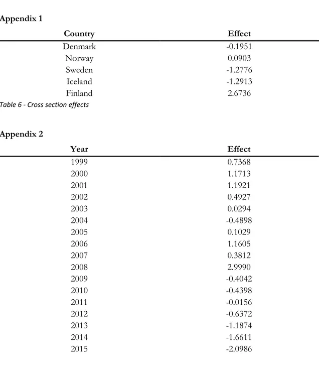
When looking at the period and country effects in the appendix, we can see that there are some trends. In the period effects, the effect is positive until 2009, when it turns to negative. In addition to that, when looking at the country effects, Finland shows the most extreme value, 2.6736, one reason behind that value could be the relatively large unemployment and inflation rate during the looked timespan.

5.2 OLS

We have also run the OLS regression to compare with the two-way fixed effects regression and the results are shown in table 6. When comparing the fixed effects results to the ordinary least squares (OLS) result, the variables are less significant than when using the fixed effects model. R-squared value is much lower, which also shows that the model is not as fitting in comparison with the fixed effects model. In both models, we can see that when removing the exchange rate from the model, the R-squared values decreased, but the decrease is higher in the case of the OLS regression. When running the original model, then only the intercept and control variables become significant. When removing the exchange rate from the model, unemployment becomes significant at one percent level, but the R square value is much lower, around 0.10. The intercept value is positive in all of the cases in the OLS regression, comparing to the fixed effects model, when the intercept value is negative in the first model. Also, the effect of unemployment on inflation is negative in the OLS model in comparison with the fixed effects results.

Table 6 - OLS regression results

Independent Variable Inflation rate Without exchange rate Without control variables Intercept 1.7586* (0.9693) 5.0618*** (0.8197) 4.0308*** (0.5145) 𝒖𝒆𝒊𝒕 -0.0140 (0.1037) -0.3222*** (0.0806) -0.3155*** (0.0809) 𝒖𝒆_𝒊𝒕𝑫_𝒕 -0.0820 (0.0693) -0.0222 (0.0625) 0.0362 (0.0617) Control variable 𝒘𝒊𝒕 -0.4938** (0.2128) -0.4940* (0.2678) - 𝒀_𝒊𝒕 -0.1609** (0.0712) -0.1095 (0.0701) - 𝒍𝒏(𝒆𝒊𝒕) -0.7626*** (0.1907) - - Observations 90 R2 _{0.33 R}2 _{0.15 R}2 _0.11 *p<0.1 **p<0.05 ***p<0.01 Robust standard errors in parentheses

6. Discussion

As mentioned previously, the original Phillips Curve has gotten critique about its applicability to today’s economy. When interpreting the results, the downsides of the Phillips Curve need to be taken into consideration. Firstly, it might be the case that Phillips Curve is not applicable for all countries, and it might be outdated for modern times. Secondly, it is also pointed out in one of the research papers, that the Phillips Curve is not stable over time and that it is not a good model for forecasting (Lucas, 1976). Furthermore, the original analysis was conducted with data from the 19th _{and 20}th _{century, making it even less convincing with}

nowadays’ data leading to our results.

The relationship between unemployment and inflation is related to the use of monetary policy as well as being affected by it (Malikane & Mokoka, 2012). Low inflation is expected from the monetary policy these five countries have applied, which is setting the inflation target at around 2%, despite it being decided by the country’s central banks. As the Phillips Curve flattens and, the relationship between the two factors decreases, the monetary policy should react more strongly to unemployment (Laseen & Taheri Sanjani, 2016). This shows that the major advanced economies had only a small decrease in the inflation rate, but a relatively large increase in unemployment. The IMF believes that the decreased responsiveness of the inflation rate is due to better and more precise inflation forecasting methods, showing the success of inflation targeting (International Monetary Fund, 2013). This alongside with globalisation, has clearly shown that the Phillips Curve has become flatter, especially for advanced economies, supporting our conclusion (IMF, 2006).

Price stability is another factor that affected the relationship. Strict controls over the price level in European Union and in the Nordic countries are set to help to keep inflation low, which is control by the European Central Bank and also by the central bank in each country (Central Bank of Iceland, n.d.) (Riksbanken, 2018) (Suomen Pankki, n.d.) (Norges Bank, 2006) (Danmarks Nationalbank, 2017).

Since our model was based on the old Phillips equation, we did not take the nominal rigidity or sticky wage into account, where wages fail to adjust to the new level. Firms are unable to cut wage due to the stickiness, leading to a reduction in the number of employment, thus increasing the unemployment rate. This situation can also be called downward nominal wage

1936). Downward nominal wage rigidities have also been indicated to be a cause of the bending Phillips Curve by Daly (2014). It has also been shown that there is a strong connection between nominal wage growth and inflation for 25 European countries through a survey done in 2014 by European Central Bank. Therefore, we can say that there is a strong connection between wage growth, inflation and unemployment, hence after removing wage growth, significant differences can be seen from the regression results.

Another crucial element is the development of Information Communication Technology (ICT) sector. Poor productivity would prevent inflation from falling, keeping the labour unit cost high, affecting wage and nominal price. However, thanks to the development of better technology in production, productivity has experienced high growth, which also lead to the relative price change in the market and wage, hence affecting the inflation rate. In the Nordic countries, the ICT sector is more concentrated than the private sector in general. In 1998, these sectors contributed 13-15% of turnover to the economy in Finland and Sweden and were a major economic importance already back then (The ICT sector in the Nordic countries, 2000). With higher productivity, the inflation rate decreased, which has also led to the negative inflation rate in Sweden and Finland as these countries are more advanced in technology, meaning less labour work is used, in contrast with Iceland, which still relies somewhat heavy on labour work for fishing.

7. Conclusion

The purpose of this thesis was to research the effect of the Great Recession upon the relationship between unemployment and inflation rate during the period between 1999 and 2016. We have found that the relationship has changed and is scarcely applicable in the present time for the Nordic countries, this result might be due to the effect of the Global Financial Crisis.

Our finding has led us to further believe that for better decision making, policymakers should not only rely on looking at this relationship. Since the trade-off between unemployment and inflation is only valid in the short run, it cannot be used to permanently lower the unemployment rate through monetary policy. This is also shown by previous studies done by Roberts (2017) and Forder (2010), on the applicability of the Phillips Curve during the time of globalization. It cannot be confirmed whether inflation and unemployment have a causal relationship or not, however, there are other elements that affects both the two variables. Monetary policy, ICT and wage stickiness are a few to mention that affect both inflation and unemployment. Hence, due to the low inflation rate, further research could focus on the NKPC in order to capture the effect of the wage stickiness. Also, a study on the effect of different monetary policy should also be considered due to the impact of it on unemployment and inflation.

In the thesis, inflation was set to be the dependent variable to capture the effects of the crisis by how other variables, such as unemployment. The study was done by looking at the period from 1999 to 2016 across five Nordic countries. Additionally, the before- and after-crisis were considered, which allowed us to fully observe the changes to the variables during and after the Global Financial Crisis. By using the fixed effects model, we could assess the net effect of the crisis on the relationship between unemployment and inflation in the Nordic countries.

8. Reference list

Andersen, T. (2007). The Nordic model. Helsinki.

Bakhshi, Z., & Ebrahimi, M. (2016). The effect of real exchange rate on unemployment.

Marketing and Branding Research, 3(1), 5. http://dx.doi.org/10.19237/MBR.2016.01.01

Baltagi, B. (2008). Econometric analysis of panel data (3rd ed., p. 165). Chichester: John Wiley.

Basistha, A., & Nelson, C. (2007). New measures of the output gap based on the forward-looking new Keynesian Phillips Curve. Journal of Monetary Economics, 54(2), 498-511.

http://dx.doi.org/10.1016/j.jmoneco.2005.07.021

Beckhart, B., & Keynes, J. (1936). The General Theory of Employment, Interest and Money. Political Science Quarterly, 51(4), 600. doi: 10.2307/2143949

Blanchard, O. (2016). The Phillips Curve: Back to the '60?. American Economic Review, 106(5), 31-34. http://dx.doi.org/10.1257/aer.p20161003

Blanchard, O., Giavazzi, F., & Amighini, A. (2010). Macroeconomics (pp. 189-190). Harlow: Prentice Hall.

Bulligan, G., & Viviano, E. (2017). Has the wage Phillips Curve changed in the euro area?. IZA Journal Of Labor Policy, 6(1), 1-5. http://dx.doi.org/10.1186/s40173-017-0087-z

Cambridge University Press. (2018). Wage-push inflation. Cambridge Dictionary. Retrieved from https://dictionary.cambridge.org/dictionary/english/wage-push-inflation

Carstensen, M. (2011). New Financial Regulation in Denmark after the Crisis – or the Politics of Not Really Doing Anything. Danish Foreign Policy Yearbook 2011, 106-129. Retrieved from https://www.diis.dk/en/research/danish-foreign-policy-yearbook-2011

Cazes, S., Verick, S., & Al Hussami, F. (2013). Why did unemployment respond so

differently to the Global Financial Crisis across countries? Insights from Okun’s Law. IZA

Journal Of Labor Policy, 2(10), 5-7. doi: 10.1186/2193-9004-2-10

Chapter III. How Has Globalization Affected Inflation?. (2006). Retrieved from

https://www.imf.org/external/pubs/ft/weo/2006/01/pdf/c3.pdf

Crespo Cuaresma, J., & Silgoner, M. (2013). Economic Growth and Inflation in Europe: A Tale of Two Thresholds. JCMS: Journal Of Common Market Studies, 52(4), 843-860.

http://dx.doi.org/10.1111/jcms.12117

Data World Bank. (2018). Exports of goods and services (current US$) | Data. Data.worldbank.org. Retrieved 13 April 2018, from

Data World Bank. (2018). GDP growth (annual %) | Data. Data World Bank. Retrieved 12 April 2018, from

https://data.worldbank.org/indicator/NY.GDP.MKTP.KD.ZG?locations=CN

Data World Bank. (2018). Imports of goods and services (current US$) | Data. Data.worldbank.org. Retrieved 13 April 2018, from

https://data.worldbank.org/indicator/NE.IMP.GNFS.CD

Dornbusch, R. (1986). Inflation, exchange rates and stabilization (p. 5). Princeton, N.J.: International Finance Section, Department of Economics, Princeton University.

Dornbusch, R., Fischer, S., & Kearney, C. (1995). Macroeconomics. Sydney: McGraw-Hill Book Co.

European Central Bank, E. Monetary Policy. European Central Bank. Retrieved 13 March 2018, from https://www.ecb.europa.eu/mopo/html/index.en.html

European Central Bank. (2014). Wage Dynamics Network (WDN). Retrieved from

https://www.ecb.europa.eu/pub/economic-research/research-networks/html/researcher_wdn.en.html

European Commission (2009). Economic crisis in Europe: Causes, Consequences and Responses. (p. 24). Luxembourg.

Evans-Pritchard, A. (2009). Thanks to the Bank it's a crisis; in the eurozone it's a total catastrophe. Telegraph.co.uk. Retrieved 18 March 2018, from

https://www.telegraph.co.uk/finance/comment/ambroseevans_pritchard/4958395/Than ks-to-the-Bank-its-a-crisis-in-the-eurozone-its-a-total-catastrophe.html

Exports to our 30 largest trade partners. (2018). Statistiska Centralbyrån. Retrieved 7 March 2018, from https://www.scb.se/en/finding-statistics/statistics-by-subject-area/trade-in-

goods-and-services/foreign-trade/foreign-trade---exports-and-imports-of-goods/pong/tables-and-graphs/exports-to-our-30-largest-trade-partners/

Fontinelle, A. (2018). Goldilocks Economy. Investopedia. Retrieved 13 March 2018, from https://www.investopedia.com/terms/g/goldilockseconomy.asp

Forder, J. (2010). Friedman's Nobel Lecture and the Phillips Curve Myth. Journal Of The History Of Economic Thought, 32(3), 330-331.

http://dx.doi.org/10.1017/s1053837210000301

Forder, J. (2014). Macroeconomics and the Phillips Curve myth (p. 3). Oxford Scholarship Online.

Friedman, M. (1968). The Role of Monetary Policy. The American Economic Review, 58(1), 1-17. Retrieved from http://www.jstor.org/stable/1831652

Fuhrer, J. (2009). Understanding inflation and the implications for monetary policy (pp. 433-444). Cambridge, MA: MIT Press.

Fuhrer, J., Kodrzycki, Y., Little, J., & Olivei, G. (2009). Understanding inflation and the implications for monetary policy (p. 6). Cambridge, MA: MIT Press.

Galí, J. (2011). THE RETURN OF THE WAGE PHILLIPS CURVE. Journal Of The

European Economic Association, 9(3), 436-461. doi: 10.1111/j.1542-4774.2011.01023.x

Gali, J., & Gertler, M. (1999). Inflation dynamics: A structural econometric analysis. Journal Of Monetary Economics, 44(2), 195-222.

http://dx.doi.org/10.1016/s0304-3932(99)00023-9

Gärtner, M. (2016). Macroeconomics (5th ed., pp. 488-490). Harlow [etc.]: Pearson. Gillman, M., Harris, M. and Mátyás, L. (2004). Inflation and growth: Explaining a negative effect.

Gordon, R. (2013). The Phillips Curve is Alive and Well: Inflation and the NAIRU During the Slow Recovery. doi: 10.3386/w19390

Gujarati, D. (2003). Basic econometrics (4th ed., p. 86). Boston: McGraw-Hill.

Gylfason, T., Holmström, B., Korkman, S., Söderström, H., & Vihriälä, V. (2010). Nordics in global crisis (p. 33). Helsinki: Research Institute of the Finnish Economy (ETLA). Imports from our 30 largest trade partners. (2018). Statistiska Centralbyrån. Retrieved 7 March 2018, from https://www.scb.se/en/finding-statistics/statistics-by-subject- area/trade-in-goods-and-services/foreign-trade/foreign-trade---exports-and-imports-of-goods/pong/tables-and-graphs/imports-from-our-30-largest-trade-partners/

Inflation, consumer prices (annual %). (2018). The World Bank. Retrieved 13 March 2018, from https://data.worldbank.org/indicator/FP.CPI.TOTL.ZG

International Monetary Fund (2013). World economic outlook, April 2013: Hopes, Realities and

Risks. (pp. 84-85). Washington DC.

Isard, W. (1954). Location Theory and Trade Theory: Short-Run Analysis. The Quarterly

Journal of Economics, 68(2), p.305.

Jochem, S. (2010). Managing the Crisis: Sweden Country Report (pp. 1-41). Gütersloh: Bertelsmann Stiftung.

Kitov, I. (2006). Inflation, Unemployment, Labour Force Change in the USA. SSRN Electronic Journal, (28), 13. http://dx.doi.org/10.2139/ssrn.886662

Kredittilsynet. (2009). The Financial Market in Norway 2008: Risk outlook. Oslo: Kredittilsynet.

Kuh, E. (1967). A Productivity Theory of Wage Levels--An Alternative to the Phillips Curve. The Review Of Economic Studies, 34(4), 333. http://dx.doi.org/10.2307/2296554

Labour Force Survey. (2018). Statistics Norway. Retrieved 13 March 2018, from

https://www.ssb.no/en/arbeid-og-lonn/statistikker/aku/kvartal

Labour Force Surveys (LFS). (2018). Statistiska Centralbyrån. Retrieved 13 March 2018, from

http://www.scb.se/en/finding-statistics/statistics-by-subject-area/labour-market/labour-force-surveys/labour-force-surveys-lfs/

Laseen, S., & Taheri Sanjani, M. (2016). Did the Global Financial Crisis Break the U.S. Phillips Curve?. IMF Working Papers, 16(126), 4,5.

http://dx.doi.org/10.5089/9781498348645.001

Law, J.(Ed.), (2014). Stagflation. A Dictionary of Finance and Banking. : Oxford University Press. Retrieved 7 Mar. 2018, from

http://www.oxfordreference.com.proxy.library.ju.se/view/10.1093/acref/9780199664931. 001.0001/acref-9780199664931-e-5674.

Laxton, D., Rose, D., & Tambakis, D. (1999). The U.S. Phillips Curve: The case for asymmetry. Journal Of Economic Dynamics And Control, 23(9-10), 1481-1482.

http://dx.doi.org/10.1016/s0165-1889(98)00080-3

Liang, Y. (2012). Global Imbalances as Root Cause of Global Financial Crisis? A Critical Analysis. Journal Of Economic Issues, 46(1), 101.

http://dx.doi.org/10.2753/jei0021-3624460104

Lin, C., Edvinsson, L., Chen, J., & Beding, T. (2014). National Intellectual Capital and the Financial Crisis in Denmark, Finland, Iceland, Norway, and Sweden. Springerbriefs In Economics, 7. http://dx.doi.org/10.1007/978-1-4614-9536-9

Lucas, R. (1976). Econometric policy evaluation: A critique. Carnegie-Rochester Conference

Series On Public Policy, 1, 19-46. http://dx.doi.org/10.1016/s0167-2231(76)80003-6

Malikane, C., & Mokoka, T. (2012). Monetary policy credibility: A Phillips Curve view. The

Quarterly Review Of Economics And Finance, 52(3), 266-271.

http://dx.doi.org/10.1016/j.qref.2012.05.002

Mankiw, N., & Reis, R. (2002). Sticky Information versus Sticky Prices: A Proposal to Replace the New Keynesian Phillips Curve. The Quarterly Journal Of Economics, 117(4), 1295-1328. http://dx.doi.org/10.1162/003355302320935034

Modigliani, F., & Papademos, L. (1975). Targets for Monetary Policy in the Coming Year. Brookings Papers On Economic Activity, 1975(1), 141.

http://dx.doi.org/10.2307/2534063

Monetary and exchange-rate policy. (2017). Danmarks Nationalbank. Retrieved 14 March 2018, from

http://www.nationalbanken.dk/en/monetarypolicy/implementation/Pages/Default.aspx

Monetary policy. (2006). Norges Bank. Retrieved 14 March 2018, from

https://www.norges-bank.no/en/about/Mandate-and-core-responsibilities/Monetary-policy-in-Norway/

Monetary Policy. Seðlabanki Íslands. Retrieved 14 March 2018, from https://www.cb.is/monetary-policy/

Monetary policy. Suomen Pankki. Retrieved 14 March 2018, from

https://www.suomenpankki.fi/en/monetary-policy/

Napolitano, O., & Montagnoli, A. (2010). The European Unemployment Gap and the Role of Monetary Policy. Economics Bulletin, 30(2), 1347. Retrieved from

http://www.accessecon.com/Pubs/EB/2010/Volume30/EB-10-V30-I2-P125.pdf

Nason, J., & Smith, G. (2008). Identifying the new Keynesian Phillips Curve. Retrieved 17 March 2018, from http://onlinelibrary.wiley.com/doi/10.1002/jae.1011/pdf

Öberg, S. (2009). Sweden and the financial crisis. Speech, Stockholm.

OECD Economic Surveys: Finland 2010: Overcoming the crisis and beyond. (2010a) (pp. 19-52). Paris.

OECD Economic Surveys: Norway 2010: Overcoming the crisis and beyond. (2010b) (pp. 19-66). Paris.

Okun, A. M. (1962). Potential GNP & Its Measurement and Significance, American Statistical Association, Proceedings of the Business and Economics Statistics Section, 98-104.

Phelps, E. (1967). Phillips Curves, Expectations of Inflation and Optimal Unemployment over Time. Economica, 34(135), 254. http://dx.doi.org/10.2307/2552025

Roberts, J. (1995). New Keynesian Economics and the Phillips Curve. Journal Of Money, Credit And Banking, 27(4), 979-980. http://dx.doi.org/10.2307/2077783

Roberts, P. (2017). Phillips Curve, R.I.P. The International Economy, 31(4), 36-37. Retrieved from

https://search.proquest.com/docview/1984836617/abstract/B83B69532C3E4800PQ/1?a ccountid=11754

Rouksar-Dussoyea, B., Ming-Kang, H., Rajeswari, R., & Yin-Fah, B. (2017). Economic Crisis in Europe: Panel Analysis of Inflation, Unemployment and Gross Domestic Product Growth Rates. International Journal Of Economics And Finance, 9(10), 147-148.

http://dx.doi.org/10.5539/ijef.v9n10p145

Rudd, J., & Whelan, K. (2001). New Tests of the New-Keynesian Phillips Curve. SSRN Electronic Journal. http://dx.doi.org/10.2139/ssrn.278442

Russell, D. (1963). Wages and Unemployment | Dean Russell. Fee.org. Retrieved 16 April 2018, from https://fee.org/articles/wages-and-unemployment/

SEB Large Corporates & Financial Institutions. (2017). Nordic Outlook (p. 14). Stockholm: Skandinaviska Enskilda Banken AB (SEB). Retrieved from

https://sebgroup.com/siteassets/large_corporates_and_institutions/prospectuses_and_do wnloads/research_reports/nordic_outlook/2017/no_1709_en.pdf

Skarica, B. (2016). Revisiting the Eurozone Phillips Curve. Economic Outlook, 40(1), 28-36. http://dx.doi.org/10.1111/1468-0319.12198

Soderstrom, U., Soderlind, P., & Vredin, A. (2005). New-Keynesian Models and Monetary Policy: A Re-examination of the Stylized Facts*. Scandinavian Journal Of Economics, 107(3), 521-546. http://dx.doi.org/10.1111/j.1467-9442.2005.00421.x

Statistics Dennmark. (2000). The ICT sector in the Nordic countries. København. Statistics Sweden (2017). Quality Declaration: Labour Force Surveys (LFS). Statistics Sweden, p.5.

Statistics Sweden. (2018). Exports to our 30 largest trade partners. Statistiska Centralbyrån. Retrieved 13 March 2018, from http://www.scb.se/en/finding-statistics/statistics-by- subject-area/trade-in-goods-and-services/foreign-trade/foreign-trade---exports-and-imports-of-goods/pong/tables-and-graphs/exports-to-our-30-largest-trade-partners/ Stiglitz, J. (1997). Reflections on the Natural Rate Hypothesis. Journal Of Economic Perspectives, 11(1), 9. http://dx.doi.org/10.1257/jep.11.1.3

Taylor, J. (1993). Discretion versus policy rules in practice. Carnegie-Rochester Conference Series

On Public Policy, 39, 200-205. http://dx.doi.org/10.1016/0167-2231(93)90009-l

Tervanen, K. (2009). Impact of Financial Crisis on the Banking Sector. International Law Office. Retrieved 17 March 2018, from

http://www.internationallawoffice.com/Newsletters/Banking/Finland/Procop-Hornborg/Impact-of-Financial-Crisis-on-the-Banking-Sector

Unemployment, total (% of total labour force). (2018). The World Bank. Retrieved 13 March 2018, from https://data.worldbank.org/indicator/SL.UEM.TOTL.NE.ZS

W.Cashell, B. (2014). Inflation and Unemployment: What is the connection? (p. 1). Federal Publications.

Wiczer, D. (2014). Are Wages and the Unemployment Rate Correlated. Stlouisfed.org. Retrieved 16 April 2018, from https://www.stlouisfed.org/on-the-economy/2014/december/are-wages-and-the-unemployment-rate-correlated

9. Appendices

Table 6 - Cross section effects

Appendix 2 Year Effect 1999 0.7368 2000 1.1713 2001 1.1921 2002 0.4927 2003 0.0294 2004 -0.4898 2005 0.1029 2006 1.1605 2007 0.3812 2008 2.9990 2009 -0.4042 2010 -0.4398 2011 -0.0156 2012 -0.6372 2013 -1.1874 2014 -1.6611 2015 -2.0986

2016 -1.3321

Table 7 - Period effects

Appendix 3

Null hypothesis: No cross-section correlation

Statistic Degrees of freedom Probability Breusch-Pagan LM test 37.4534 10 0.0000