Analysis of the process-induced piping defect in extrusion with conical discs, An

AN ANALYSIS OF THE PROCESS-INDUCED PIPING DEFECT IN EXTRUSION WITH CONICAL DIES

by

All rights reserved INFORMATION TO ALL USERS

The qu ality of this repro d u ctio n is d e p e n d e n t upon the q u ality of the copy subm itted. In the unlikely e v e n t that the a u th o r did not send a c o m p le te m anuscript and there are missing pages, these will be note d . Also, if m aterial had to be rem oved,

a n o te will in d ica te the deletion.

uest

Published by ProQuest LLC(2018). C op yrig ht of the Dissertation is held by the Author.

All rights reserved.

This work is protected against unauthorized copying under Title 17, United States C o d e M icroform Edition © ProQuest LLC.

ProQuest LLC.

789 East Eisenhower Parkway P.O. Box 1346

A thesis submitted to the Faculty and the Board of Trustees of the Colorado School of Mines in partial fulfillment of the requirements for the degree of Master of Science

(Metallurgical and Materials Engineering).

Golden, Colorado . H i ! D a t e : Signed Gokhan Erdem Approved:

Dr. C.&K Van Tyne Thesis Advisor Golden, Colorado D a t e : M I M f t ---Dr{/ John J. Moore

Professor and Department Head, Department of

Metallurgical and Materials Engineering

ABSTRACT

The piping defect which can occur near the end of the stroke in the extrusion process with conical dies has been modeled by applying the upper bound approach and the finite element method. The influence of the process conditions such as billet length, die angle, radius, and reduction ratio on the formation of piping defect is presented.

For the extrusion process both with and without a pipe, kinematically admissible velocity patterns have been

developed and analyzed by the upper bound approach. The analyses divide the workpiece into four zones separated by three surfaces of velocity discontinuity. The power terms are calculated for each zone separately and the formation of the piping defect is investigated. The results which were obtained from the upper bound method were used to determine criteria for the occurrence of the piping defect as a

function of the major process parameters. It is observed that decreasing the billet length, increasing the die angle, increasing the product radius and increasing the non-angled portion of the die cause an increased potential for

formation of the piping defect. Although the friction causes a large increase in the required extrusion pressure,

an increase in the friction factor increases the domain for piping by a small amount.

The extrusion process is also analyzed by the finite element method (FEM). The results obtained from the upper bound approach have been correlated to the results from the finite element method. The finite element method exhibits reasonable agreement with the upper bound model for both the prediction of pipe size and the criteria curve for the

prevention of the piping defect.

TABLE OF CONTENTS

page

ABSTRACT ... iii

TABLE OF CONTENTS ... V LIST OF FIGURES ... vii

LIST OF TABLES ... x

NOMENCLATURE ... xi

ACKNOWLEDGMENTS ... xiv

1. INTRODUCTION ... 1

2. BACKGROUND ... 14

2.1 THE UPPER BOUND APPROACH ... 14

2.2 THE FINITE ELEMENT METHOD IN METAL FORMING PROCESS MODELING ... 23

3. OBJECTIVE OF STUDY ... 27

4. ANALYSIS OF THE PROCESS ... 29

4.1 UPPER BOUND ANALYSIS ... 29

4.2 FINITE ELEMENT ANALYSIS ... 49

5. RESULTS AND DISCUSSION ... 53

5.1 UPPER BOUND ANALYSIS.... ... 53

5.1.1 Characteristics of the Process ... 54

5.1.2 Criteria Curves for Defect Prevention ... 67

5.2 FINITE ELEMENT METHOD ANALYSIS ... 77

6. CONCLUSIONS ... 84

REFERENCES ... 85

APPENDIX I ... 88

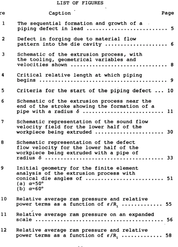
LIST OF FIGURES

Figure Caption Page

1 The sequential formation and growth of a

piping defect in lead ... 5 2 Defect in forging due to material flow

pattern into the die cavity ... 6 3 Schematic of the extrusion process, with

the tooling, geometrical variables and

velocities shown ... . ... 8 4 Critical relative length at which piping

begins ... ... 9 5 Criteria for the start of the piping defect ... 10 6 Schematic of the extrusion process near the

end of the stroke showing the formation of a

pipe with a radius 6 ... 11 7 Schematic representation of the sound flow

velocity field for the lower half of the

workpiece being extruded ... 30 8 Schematic representation of the defect

flow velocity for the lower half of the workpiece being extruded with a pipe of

radius 6 ... 33 9 Initial geometry for the finite element

analysis of the extrusion process with

conical die angles of ... 51 (a) a=50°

(b) a=60°

10 Relative average ram pressure and relative

power terms as a function of e/R± ... 55 11 Relative average ram pressure on an expanded

scale ... 56 12 Relative average ram pressure and relative

power terms as a function of e/R± ... 58 vii

13 Relative average ram pressure on an expanded

scale ... 59 14 Relative average ram pressure at the

transition point between sound flow and

defect flow ... 61 15 The relative pipe size as a function of

relative length of the non extruded portion

of the billet for a die angle a=7 5 ° ... 63 16 The relative pipe size as a function of

relative length of the non extruded portion

of the billet for a die angle a = 6 0 ° ... 64 17 The relative pipe size as a function of

relative length of the non extruded portion

of the billet for a die angle a = 4 5 ° ... 65 18 Criteria curve for piping defect formation .... 68 19 Criteria curve for piping defect formation .... 69 20 Criteria curve for piping defect formation .... 70 21 Criteria curve as a function of the relative

length of the non extruded portion of the billet and the relative radius of the

conical region of the die ... 73 22 Criteria curve as a function of the relative

length of the non extruded portion of the

billet and the inverse reduction ratio ... 74 23 The formation of piping defect for a=50°

using NIKE2D, ... 78 (a) Full view, and

(b) an expanded scale

24 The formation of piping defect for a=60°

using NIKE2D, ... 79

(a) Full view, and (b) an expanded scale

25 Comparison of relative pipe size as determined by the finite element

method and the upper bound approach ... 80 26 Comparison for occurrence of a pipe as

determined by the finite element method

and the upper bound approach ... 82

LIST OF TABLES

Table Caption Page

1 The specific material properties used in the

finite element analysis ... 52

NOMENCLATURE A = dimensionless function B = dimensionless function e = dimensionless function E = Young's modulus f = dimensionless function J* = upper bound on power k = Mises' yield constant

L = length of the non extruded portion of the billet

m = constant friction factor p = dimensionless function Pave = average ram pressure q = dimensionless function

R = cylindrical coordinate in radial direction Ra = radius of the angled portion of the die Ri = product radius

R _O = ram radius S = surface

Sr. = surface of velocity discontinuity t = time

T± = external traction

U = velocity of ram

UR = radial component of velocity Uy = axial component of velocity

\Jg = circumferential component of velocity v± = velocity

V = volume

V = slope of W(R) as a function of R V = slope of Z(R) as a function of R Av = tangential velocity difference

W(R) = axial position of die face as a function of R Wi = internal power of deformation

Ws = shear power losses

Wf = frictional power losses

y = cylindrical coordinate in axial direction

Z (R) = axial position of r3 surface as a function of R a = conical die angle

/3 = dimensionless function V = dimensionless function

6 = crack length (a pseudo-independent parameter)

e = position of T3 surface on axis of symmetry (a pseudo-independent parameter)

e.. = strain rate

p = dimensionless radial position variable

direction shear stress

ACKNOWLEDGEMENT

I am very thankful to Dr. Chester J. Van Tyne, my thesis advisor, for his guidance, patience, valuable discussions, and helpful comments during my research at Colorado School of Mines.

It is a pleasure to express my deep gratitude to Dr. George Krauss and Dr. Robert H. Frost for serving as members on the committee and their assistance to this study.

For financial support throughout this research, I would like to thank Eregli Iron and Steel Inc. Partial support of a portion of this work by the AMAX Foundation is gratefully acknowledged.

Special thanks are due to Mr. W.A. Gordon of Torrington Company for interest in my research.

Finally, I owe a considerable debt to my family who provided help and understanding in a great number of w a y s . Especially, I would like to thank to my grandmother Hayriye Tetik, my father Abdurrahman Erdem and my mother Ozden Erdem

for their love and support.

1.INTRODUCTION

Metal deformation processes can be viewed as systems with a large number of interacting variables such as

material properties of the workpiece and the tooling,

tribological conditions in the contact zone between the work piece and tools, the tool geometry, process temperature, velocity, etc. In metal forming, the prediction of metal flow is a very important consideration under a given set of processing conditions. Thus, many metal forming models require a good understanding of the interaction between these parameters in order to operate actual processes with optimal metal flow.

The modeling of metal forming processes can be considered as a key to improved product quality and

optimized production. The primary reason for using a model is that it can yield information about the actual process, which would be inaccessible or expensive to provide without the model (1). The other aim of a model is the generation of quantitative statements concerning the process

parameters. This quantification can be used to determine the optimal manufacturing conditions for a forging or extrusion. The results generated by the model should be more readily accessible, less costly or more complete than can be

obtained by laboratory experiments or tests during actual manufacturing. Clearly, the need for the development of process models is particularly great in situations where it is technically difficult to measure the process parameters in question. When complicated die geometry, complex

material characteristics, including work hardening,

tribological conditions, etc. are considered, mathematically exact solutions for the actual metal forming become very difficult, if not impossible.

Many idealized models (1-5) are usually assumed to find approximate solutions to real metal forming problems. Among the various approximation methods for solution, limit

analysis (3,4) is an analytical approach often used for metal forming operations. Two separate solutions are

developed: one is the upper bound solution, which provides a value for the required power that is equal or greater than the actual power and the other one is the lower bound

solution, which provides a value that is equal or lower than actual power. Hence, the actual value is bracketed between the two limits.

When applying the upper bound approach, the first step of the investigation is to assume a velocity field for the deforming body. Velocity can be measured directly or it can sometimes be observed in model experiments. For a lower

bound solution, however, the first step is the formulation of a stress tensor, which is far more difficult to conceive and can be measured only indirectly from experimentation. Therefore, the upper bound approach is used more often for theoretical analysis of metal forming processes.

The upper bound method considers kinematically

admissible velocity fields (i.e. those which satisfy the incompressibility requirement and the velocity boundary conditions). From the velocity field the internal power of deformation, the internal shear power losses and the

frictional power losses are computed and summed to determine the total power required for deformation. From the

knowledge of the total forming power and the tooling geometry and velocity, the instantaneous forming load or averaged forming pressure can be determined.

An upper bound solution can provide information about the effect each individual process parameter has on the loads required for the actual manufacturing process. More important, the upper bound method coupled with principle of minimum energy can be used to indicate process conditions which might produce a defect during metal forming operations

(4,7-9). A piping defect, which can occur during forging or extrusions, is produced because the flow associated with such defect formation is energetically more favorable under

the given process conditions than sound flow. The

prediction of piping defect is a matter of establishing under what conditions the energy for defect formation is less than that for sound flow.

The work presented in this study analyzes the piping defect in extrusions. Figure 1 shows the formation and growth of an actual piping defect in lead (10). The formation of the piping defect is not desirable. A

considerable portion of the material can be rendered useless in the extruded product because of it. Knowledge of the processing conditions which cause this type defect will aid the design engineer considerably, by providing reliable information about the non-defect processing requirements without expensive, time-consuming laboratory and plant-scale experiments.

In addition to the piping defect in extrusions, a similar type of defect can occur in forgings due to the material flow away from a die face (see Figure 2). This type of flow produces a cavity similar to a pipe and it is known in the forging industry as the extrusion defect (11). The results from the present work on extrusion can be

judiciously applied to forging processes so that this type of defect can be avoided.

Cn c •H a •H 04 <o 4-1 o .C -p s o u O' T3 3 <d c o •H ■p CO . e — M O O •—1 4-1 W •H T3 <d •H 0) ■P — I e Q> 3 3 CT 0 x> m u 0 Q) 4-1 .30 Eh *o 0 P 3 O' •H EH

C

av

it

schematically shown in Figure 3. The initial billet is a cylinder of radius R0. The billet is in contact with the chamber wall. The length of this contact is L which is also the length of the non extruded portion of the billet. In the extrusion process understudy, the ram pushes on the back side of the billet with a velocity U. A rod of radius Rj exits the extrusion die with a velocity vf.

Figure 4 shows the criteria developed by Avitzur. The critical relative length when piping begins for three

constant friction factor, m, can be seen. Figure 5

illustrates the criteria for the start of the piping defect developed by Gordon and Van Tyne.

Near the end of the stroke in a extrusion process, a cavity can be produced at the back end of the billet. The billet material along the axis of symmetry is moving forward more rapidly than the ram and a separation occurs (see

Figure 6). This cavity is termed a pipe since the product is a tube or a pipe rather than a solid rod. When the piping cavity starts the extrusion process should be stopped so that no defective product is produced (8).

There have been several analyses of the piping defect by other investigators. Johnson established a very simple criteria for the piping defect in a plane strain extrusion process (12,13). He indicates that a pipe will form when

Chamber o F i g u r e 3 S c h e m a t i c of th e e x t r u s i o n p r o c e s s , w i t h th e t o o l i n g , g e o m e t r i c a l v a r i a b l e s an d v e l o c i t i e s

0 .1 0

CH/l)

i»UT8 •AfV*im

Chamber CL >x F i g u r e 6 S c h e m a t i c of th e e x t r u s i o n p r o c e s s n e a r th e end th e s t r o k e s h o w i n g th e f o r m a t i o n of a p i p e w i t h

the product width is larger than one half the length of the non extruded part of the billet. In the present analysis this would be equilavent to Rj > L. Avitzur (3) has used the upper bound approach to analyze the piping defect. His analysis uses a two zone velocity field. The die has a conical region of angle a and radius Ra. A three zone velocity field has been used by Gordon and Van Tyne (8) to examine the piping defect at the end of the stroke in

extrusions with flat dies (i.e. a = 90°). This study uses a four zone velocity field and the upper bound approach to examine the formation of a pipe in an extrusion with a conical die.

This study uses another powerful mathematical technique called the finite element method (FEM) to examine the

formation of pipe. The FEM program utilized in this work is NIKE2D which is an implicit finite deformation formulation developed by J.O. Hallquist at the Lawrence Livermore

National Laboratory (14). NIKE2D uses the interactive preprocessor program called MAZE and the interactive post­ processor called ORION (15-16). The primary focus of an FEM analysis for plastic deformation is on the internal stress and strain states that the workpiece experiences during the forming operation. The upper bound approach which is based on energy balance technique cannot provide these stress and

strain states. The most notable disadvantage of the finite element analysis are the inaccuracy of the derivatives of the approximated solution, the difficulty in imposing the boundary conditions along nonstraight boundaries, the

difficulty in accurately representing geometrically complex domains, and the inability to employ nonuniform and

nonrectangular meshes (17). In this study the reason for the FEM analysis is primarily to confirm the results which are determined from the upper bound method.

2. BACKGROUND

2.1 THE UPPER BOUND APPROACH

In general, because of the complexity of the

mathematics, exact analytical solutions for metal forming processes and operations are extremely difficult, and, at present approximations and simplifying assumptions are inevitable. Analytical models rely on the closed-form solution of the plasticity equations to obtain information about forming loads, tool-workpiece interface pressure

distributions, etc. These methods are typically applicable only for the simplest of geometries and boundary

conditions (18). There are several requirements for exact analytical solutions and they can be obtained only by

following strict rules to satisfy completely a predetermined set of conditions (3-5). The requirements:

1. The equations of equilibrium for the stress tensor must be satisfied throughout the deforming body.

2. Continuity of flow must be maintained; that is, volume constancy must be satisfied.

3. The relationship between internal stresses and flow in the real material must be known and obeyed.

4. The geometric and static boundary conditions must be satisfied, including friction behavior over the indent

interface between the tool and the workpiece.

When all of the above conditions are satisfied, the solution completely and uniquely determines the state of the stress and the state of strain throughout the entire

workpiece and over its boundaries. Because of the complexity of these restrictions and the nature of the equations, there is no set prescription for obtaining a complete solution. In fact, there is not presently

available one complete solution for the unique stress and strain fields in the workpiece of any metal-forming process. However, when an upper bound solution is developed, some of the exact conditions are satisfied, while others are relaxed

(3-5). By relaxing several of the necessary conditions, the upper bound solution loses its uniqueness. For an upper bound solution, the requirements are relaxed to the extent that the equations of equilibrium, the stress-strain

relationship, and the stress-boundary conditions are not necessarily satisfied. An infinite number of flow patterns can satisfy the relaxed conditions for an upper bound

solution. The actual solution will be one which provides the lowest upper bound.

The upper bound approach often uses a simplified

version of material behavior. Although this is not totally realistic, it does reasonablely approximate the material

properties of metals which are being hot worked. If this simplification were not used, then the equations used by the upper bound would be too complex to be solved mathematically negating the possibility of a solution being determined.

The workpiece material is also assumed to be homogenous and isotropic. Therefore, the effects of strain hardening,

strain rate hardening and/or strain induced softening on the flow stress are ignored. The deviatoric stress tensor for a Mises material is related to the strain rate tensor in such a manner that if all strain rate components are changed proportionately, the deviatoric stress components remain unchanged (3-5).

A description of the upper bound approach as an

application of limit analysis to metal forming processes is presented by Avitzur (4). The upper bound theorem

formulated by Prager and Hodge (19) states that of all kinematically admissible strain rate fields, the one that occurs, minimizes the expression:

where J* is the upper bound on power,

k is the shear yield strength of the material,

e is a strain rate component,

V is the volume of the deforming material, T. is an external traction,

vi is a velocity component, and

St is the surface over which the traction is exerted.

In this approach, since the material is assumed to be a perfectly plastic material, which obeys the Mises stress- strain rate relation, (i.e. no volumetric change and no work-hardening), the relationship between the shear yield strength and the flow strength of the material, ao, is

a

k = — (2)

When Eq. (2) is substituted into Eq. (1), the upper bound equation becomes:

T± vA dS (3)

The first term on the right side of Eq. (3) is the internal power of deformation, and the second term is the power required to overcome external tractions, T±, opposing the deformation process.

In metal forming operations, shear power along surfaces of velocity discontinuity within the deforming workpiece and frictional power loses between the tool and the workpiece need to be included. These additions presented by Drucker

(20), modify Eq. (3) to become:

(4) + rf | AV| dS - T. v ^ S

where r is the internal shear stress,_{S '}

rf is the frictional stress on the interface, Sri is a surface of velocity discontinuity within

the deforming workpiece, and

Sr2 is a surface between the tool and the workpiece where friction is present.

This form of the equation has been used extensively for upper bound solutions of metal forming processes. The first term on the left side of Eq. (4) represents the power for internal deformation over the volume of the deforming body. The second term includes all the shear power losses over internal surfaces of velocity discontinuity. The third term includes the power losses due to friction between the

tooling and the workpiece and the last term is the power supplied to overcome any external tractions.

In the upper bound approach, because the body is fully plastic, the friction is usually described by the constant friction factor formulation. This relationship is assumed to occur at all workpiece-tool interfaces. Therefore, the friction stress is

m a.

(5)

where m is the constant friction factor.

die, workpiece, and lubricant under constant surface and temperature conditions (3-6,21). It has values between 0.0 for frictionless conditions and 1.0 for sticking friction.

In order to analyze a metal flow process by applying the upper bound analysis, it is necessary to make several assumptions and to perform the following steps (3-6).

1. Assume a velocity field which satisfies the conditions of incompressibility and the velocity boundary

conditions.

2. Calculate the energy rates for deformation such as the internal power of deformation, the frictional power losses, the internal shear power losses etc.

3. Determine the total energy, J*.

4. Assume another velocity field and find if it produces a lower J*.

This process continues until the lowest J* is determined.

The deformation load for the process can be obtained by dividing the energy rate by the normal velocity of the die acting on the workpiece. The total energy rate, J*, can be expressed as

J* = W + W + W

internal shear friction ( 6 )

By the upper bound theorem (3-4), the load calculated will be greater than the actual load and hence represent an upper bound to the actual forming load. When the upper bound load becomes lower, the prediction becomes better.

In order to examine a large number of flow patterns at the same time, the velocity field may contain an extra

parameter. This parameter is often used to determine the position of one of the internal surfaces of velocity

discontinuity. The value of this parameter, which minimizes the total power of deformation, is the one that provides the most realistic velocity field. This parameter can also be used to determine whether or not a defect would exist under a given set of process conditions. Although this parameter is initially considered as an independent variable, it is not truly independent since its value is determined by minimizing the total power. Because of the dual

characteristic of independency and dependency, this variable is classified as a pseudo-independent parameter.

Often, the flow pattern for deformation processes

includes one or more pseudo-independent parameters (4) whose values are determined by minimizing the total energy rate, J*, with respect to such parameters. When the number of pseudo-independent parameters increases in the flow pattern, the solution improves, but the mathematical computations

become more complex. More detailed information about the use of a pseudo-independent parameter for the determination of the pipe defect in extrusions is given in Section 4.

2.2. THE FINITE ELEMENT METHOD IN METAL FORMING PROCESS MODELING

Process modeling for deformation mechanics has been a major concern in metal working technology. Proper design and control of metal forming processes requires global as well as local knowledge of the mechanics during deformation. Several analytical techniques are available which simulate the forming of metals. As computers become increasingly efficient, the numerical modeling of metal forming processes is an attractive and economical means of understanding a variety of metal working operation (22).

The finite element method (FEM) is a powerful technique for determining stresses and displacements in deforming

workpiece too complex for strictly analytical methods. Indeed the finite element process is established as a general numerical method for solutions of partial

differential equation systems, subject to known boundary and/or initial conditions (17). This method has found

greater usage in engineering practice due to the common use of computer graphics and availability of powerful computer workstations. The finite element method appeared in the metal forming field in the early 1970s. When this method was introduced for the analyses of metal forming processes, accurate determination of the effects of various parameters

involved in the processes in the detailed metal flow became possible (23). The first applications of the finite element analysis utilized infinitesimal elasto-plastic formulations for small deformations (24,25) and soon it became evident that metal forming required greater sophistication.

In order to simulate metal flow during a deformation process by the finite element method, a number of finite points are identified in the domain of the workpiece. These points are called nodal points. The domain of the function being sought is represented approximately by a finite

collection of subdomains called finite elements. The domain then is composed of an assemblage of elements connected

together appropriately within each element by continuous functions which are uniquely described in terms of the nodal point values associated with the particular element. The basis of finite element metal flow modeling, using the variational approach, is to formulate proper functionals, depending upon specific constitutive relations. The

solution of the original boundary value problem is obtained by the solution of dual variational problem where the first- order variation of the functional vanishes. An approximate interpolation function for the field variable is used within these elements. The functional is expressed locally within each element in terms of the nodal points. The local

element equations are then assembled into the overall

problem. Thus, the functional is approximated by a function of global nodal point values (23).

In many metal forming operations, the geometry of the workpiece changes with time. Part of the surface that was

free may come in contact with the tooling, becoming

restricted in the normal direction with frictional forces applied in the tangential direction. The possibility of defining one or more dies, moving or not, with arbitrary shape, together with all geometric verifications and adoptions, requires sophisticated programming. These

procedures can be done by commercial finite element programs which have pre- and post-processors (26).

The advancements in the application of the finite element method have been mainly toward expanding its

applicability to a variety of metal forming processes. With continual effort on improving the finite element technique, this method has became a most powerful theoretical tool in analyzing metal forming problems. Recently, the finite element method has been used to calculate parameters that change locally with deformation, such as, the parameters used in damage rules (27,28). Almost all FEM applications so far have dealt with two dimensional problems, but this method will undoubtedly be extended to three-dimensional

3. OBJECTIVE OF STUDY

The axisymmetric extrusion process examined in this investigation is used to produce a cylindrical rod. This study models the process by dividing the workpiece into four deformation regions. Both sound flow and defect flow

patterns are analyzed. The criteria for the occurrence of the piping defect as a function of the process parameters for extrusion through conical dies is developed based on an upper bound approach. The criteria separate regions of sound flow from regions where piping would most likely occur.

The reason for using the upper bound approach is that there is no available method for finding exact analytical solutions in metal forming operations, and more importantly, the upper bound approach coupled with the principle of

minimum energy can be used to indicate the conditions when piping would occur.

The goal of the present study is to determine the

process parameters such as billet geometry, tooling design, and friction conditions which induce a pipe. This knowledge will provide a means of understanding the process and allows the optimal manufacturing conditions without the cost and time involved with the traditional trial and time error investigation.

In addition to the upper bound approach, the finite element method is applied to the extrusion process. The relative pipe size and the first appearance of a pipe are determined by the finite element method. The finite element method results are used to verify the results obtained from the upper bound method.

4. ANALYSIS OF THE PROCESS

4.1 UPPER BOUND ANALYSIS

The process to be analyzed is shown in Figures 3 and 6. The cylindrical coordinate system (R,0,y) is assumed to have the y axis along the axis of symmetry and the origin is

fixed to the left end of the billet. The billet is assumed to be a Mises material with a flow stress o . _o The initial cylindrical billet begins with a radius Ro. The non

extruded portion of the billet has a length L. The ram pushes on the back side of the billet with a velocity 0. The cylindrical product exits the extrusion die with a velocity vf. The radius of the product is R±. The

extrusion die has a conical region of radius Ra and angle a. A schematic representation of one half of the process is given in Figure 7. The workpiece is divided into four zones. Zone I is the outer portion of the billet and it is a ring element of inner radius Ra/ outer radius Ro and

thickness L. The side of zone I adjacent to the rams moves in the same direction as the ram with velocity 0. Zone IV is the product and it is assumed to be rigid body which moves with a velocity vf. Zone III is a complex-shaped region in which both axial and radial flow are occurring. Material deformation is occurring in zone III. Zone II is

o if) d> U 0) •H Q* M P O * d) A ■P T3 C M-l 3 o o 10 *w d) a ■p M-l o c o •H .p (0 ■P c a) <D £ -p p o CO *w 0) P T3 CU»—I 0) a) P -H M-t u •H (0 £ a) £ u cn +j •H u o «H d) > •d 0) •d 3 p -p X CD O' c •H d) A d> P 3 O' • H En

similar to zone III and there is also material deformation in this zone. The volumes of zone II, zone III and zone IV are all dependent on the die angle a and a pseudo­

independent parameter, e, whose value changes with the other process variables. In order to use the upper bound

approach, the velocity fields must be determined for each zone.

As seen in Figure 7, Sa is the interfacial surface between zone II and the die. SK is the inter facial surface between zone I and the die. S is the interfacial surface_C between zone I and the chamber. S., is the inter _a facial surface between zone I and the ram. S is the interfacial_e surface between zone II and the ram. Sf is the interfacial surface between zone III and the ram.

The four zones are separated by three surfaces of

velocity discontinuity. Surface T1 is a cylindrical surface which separates zone I from zone II. The surface is fixed at the radial position Ra. Surface T2, which separates zone II and zone III, is also a cylindrical surface, bit at the radial position R±. The surface r3, which is assumed to be a conical surface, between zone III and zone IV is shown as a linear function in Figure 7. Its exact position is

variable, depending on the pseudo-independent parameter s. The actual value that e possesses is determined through the

material will be deformed to produce a sound flow. If the optimal value of e is negative, then separation between the billet and the ram will occur. A schematic representation of this case is shown in Figure 8. When the billet material along the axis of symmetry moves forward more rapidly than the ram, a cavity occurs which is termed a pipe since the product is a tube or a pipe. Therefore, the value of e can be used to determined whether or not, for a set of geometric and process conditions, piping would occur. If the piping cavity were present the radius of the pipe would be given by the value 6 as illustrated in Figure 8.

The axial location of the T3 surface can be expressed as a function of the radial component, R. If Z is the axial position of T3, then for e > 0, the relative axial position

ox GO rx CO cn C •H (D XX 0 5 u o 0 1—1•H P 04 M P U U O 0 z P 0 0 T3 .c • ■p «o 0 XX P 10 p o 3 •H p p *0 O «H 03 03 P C XX o P •H U O p 0 03 S 0 P o 04 C r—t •P 0 04 0 0 0 XX 03 O p 04 XX 0 U P U o •H p U •H >iT3 P P 0 03 •H T3 e U 3 0 O P XX rH P u 0 X w > 0 00 0 O 3 cn •H t-i

where

For any constant value of 0, this is an equation of straight line, which is to be expected since r3 is a conical surface.

If e < 0, then the axial position of r3 as a function of R can be expressed in terms of 6. In this case

Z

K

jl R c ___

R0 R± i

-(9)

The values of e and 6 are also related to one another. Such a relationship is shown graphically in Figure 8. This relationship can be expressed mathematically by using the point where p = 0. At this point Z = e and substituting

_6 Ri i 1

-R i

(10)

In order to obtain 6 as a function of e, Eq. (10) can be rearranged, yielding _6 R, e E Ri R o R i (1 1)

The derivations of the velocity fields and the power terms for each zone are presented in Appendix I . A summary of this work is presented below. The equations for defect flow using the pseudo-independent parameter 6 will be

presented below. The equivalent equations for sound flow using e can be obtained by substitution of Eq. (11) in the equations that follow. The final equation for the ram pressure is a function of process geometry, frictional conditions and the pseudo-independent parameter.

The velocity field for each zone is calculated in cylindrical coordinates. The velocity field for each zone

is as follow: For zone I U = - UR R 2L v R '( — )2 Uy = U(1 - |) - 1 (1 2 )

This is an equivalent velocity field to the one presented by Avitzur and Van Tyne (29) in their analysis of ring forming.

For zone II u = -H ff R 2W ( — v R ')2 - 1 U = U_y 1 - I W 1 R dVI 1 2WcfR ( - ° ) 2 v R ' (13) U« = 0 where

Z = Z Z ° + cot«(l* - Z )

(14)

of the die surface (i.e. Sa in Figure 7). For zone III

u = -H ? R 2Z 6,2 1 - (i ) R_ ( — ) - 1 Ri 6,2 1 " (i ) U = U_y 1

+

This is equivalent to the velocity field for a similarly shaped zone as presented by Gordon and Van Tyne (8).

For zone IV Ur = 0 U y = v f U Rc R (_?)* - ( * )2 (16) 6 ,2 U„ = 0

of deformation for a perfectly plastic material is determined from the following equation:

r 20

"i ■ J,

-& N

^ * dv

(17)

where V is the volume of the material, and, the s is a strain rate component.

For zone I, the internal power of deformation is

W« = R22

-K A

3 (T a)4 + 1

(18)

+ In

This is the equivalent internal power of deformation as the one presented for ring forming by Avitzur and Van Tyne (29).

For zone II

VI1 = — rrUR2

P a/Rl J?

11 Jl 2 s/l + B + Bln 1 + ^ + B i/b J. pdp (19) where B ( f + 2 + Y ) + f + ( 2 + y ) p V 2 (2 0 ) and p = 2 y V „ + (f + 4)V„ -

av„

p = t

aw

H

_{11 w}

This power term requires a numerical integration to obtain a specific value for it as a function of the process

parameters.

For zone III

Lm ( — ) - 1 Ri i - (^-)2

q

av

with ' - i V = az v i i i 7 5d dR (26) e = 1 - i ( — )2 p2 ^ Rt fi = p e V m -J

This internal power of deformation is equivalent to the one presented by Gordon and Van Tyne (8 ) for a similarly shaped zone. A numerical integrations is required to solve for values of this power term.

Zone IV is assumed to move as a rigid body, therefore there is no deformation and no internal power of deformation in this zone.

There are internal shear losses along the surfaces of velocity discontinuity. These power losses can be

calculated by the following equation:

Ws = f ^ | A v | d S JSr \[3

where Sr is the surface between the two regions, and,

Av is the tangential velocity difference that exists along the surfaces.

For the surface r i# between zone I and zone II,

For the surface r2, between zone II and zone III

r r. ^)2 - 1 i 2 (29) - ( -cota - VrlI|Ei)

where

v I = L +(R* “ R i ) c o t a

111 1 Ri

----For the surface r3, between zone III and zone IV,

Wc

=jr

-(R'

1)2

\j

l + v:

l - Jlvli - (i)2'

R

A

The friction power losses along a workpiece/tool interface can be determined from the following equation:

where m is the constant friction factor,

Av is tangential velocity difference between the tool and the workpiece and S is the interfacial surface. The friction power losses along Sa, between zone II and the die are

(33) 2 • In . + _ ( ) l7Wq 2 v cota' (34) cota 1, l/r, 2 cota

The friction power losses along Sb, between zone I and the die are mo n . 2 W. = 1 _ U R{ — ) 1/3 Rc L 1 -3 R„ + i ( ^ f )33 R„ (35)

The friction power losses along Sc/ between zone I and the chamber are

W f = !!^?nlJR2(il)

y[3 R°

(36)

The friction power losses along Sd, between zone I and the ram, are equal to the frictional power losses along surface Sb. Therefore,

mo.

W f = -TTU R ( _ )

d v j R°

The friction power losses along Se, between zone II and the ram are

mcr/T . 2 W, = UR* tana & L 1 - ( tana + _*) In L R a Ri — tana + ( — - -i) Rn _o v R _o R_o -ttana R„ + 3-ttana( R0 o R0o R1 (38) 1 R. Rj , R_ R_ Rj + i ( _ I - -1)2 + 2 — (— - — ) 2 R_ _o R_ _o R_ R_ _{o o} R__o

The friction power losses along Sf/ between zone III and the ram are

m — in UR" ( — )3i_{O ' D 7 O}Ri R„ R (39) 1 * ( _ ) 2 Ri R R, __ + (— - _i)cota

The upper bound on power is

J* = w, + w, + w, + wq + w„ + w*.

AI rl r2 r3 (40)

+ VL + VL + VL + VL + VL + VL

The total power requirement for the process is supplied by the moving ram. Instead of presenting the influence a change in a process variable has on the value of the J*, it is more meaningful to relate J* to the ram pressure and show how the ram pressure is affected. This relationship can be expressed mathematically, as,

(41)

J* = U n p AVERQ2

where pAVE is the average ram pressure.

By equating Eq. (41) to the sum of the internal powers of deformation, internal shear power loses and the

frictional power loses, the relative average ram pressure can be determined. This would be

A V E J* U n R ‘ (42) or in function form = _ , a , m , & — ) Rj. R0 Rq Ri

The above function form shows that the relative average ram pressure is dependent on the geometry of the billet and tooling, the frictional conditions and the pseudo­

4.2 FINITE ELEMENT ANALYSIS

This study uses the finite element code NIKE2D which was developed by Hallquist. NIKE2D is a vectorized

implicit, finite deformation, large strain, finite element code for analyzing the response of two-dimensional

axisymmetric, plane strain, and plane stress solids (14). A variety of loading conditions can be handled including

traction boundary conditions, displacement boundary conditions, concentrated nodal points loads, body force

loads due to base accelerations, and body force loads due to spinning. NIKE2D has been applied to a wide range of large deformation, inelastic response calculations, by a number of users and generally, the results have been quite

satisfactory.

MAZE (15) is an interactive program that has been

developed as a input generator for NIKE2D. This program is used in the present work as the preprocessor for NIKE2D.

ORION (16) is the interactive color post-processor for NIKE2D. ORION reads the binary plot files generated by NIKE2D and plots contours, time histories, and deformed shapes. ORION also can compute strain measures, interfaces pressures along constrained boundaries, and momentum. This post-processor is also utilized in the present work.

The initial geometry which is used in the finite

element analysis for the billet and the tooling is shown in Figure 9. The views are cross sections through the three dimensional axisymmetric process. The orientation of the process has been rotated 90° as compared to the schematic shown in Figures 3 and 6 . The ram is at the top the diagram and the die is at the bottom . The extrusion is in the

downward direction. Different conical die angles are used in the FEM simulations. A die angle of 50° is shown in Figure 9a and an angle of 60° is shown in Figure 9b. For this process, a 50 x 15 rectangular element mesh is used to model the workpiece.

In the finite element model, the material properties need to be defined. An elastic-plastic behavior for the workpiece and an elastic behavior for the ram and chamber are assumed. The specific material properties which are used in the finite element method are given Table 1. These properties are representative of steel for tooling and hot- worked aluminum for the workpiece.

The finite element code NIKE2D uses the Coulombic friction coefficient (p) to model the interaction between the workpiece and the tool at frictional surfaces. The upper bound analysis uses the constant friction factor (m) for modeling frictional conditions.

0) -D

E

c

c

•H a\ C N o\ C N n •H O O C O O ■P in T a b l e 1 T h e s p e c i f i c m a t e r i a l p r o p e r t i e s u s e d in the f i n i t e e l e m e n t a na l ys i s.

5. RESULTS AND DISCUSSION

5.1 UPPER BOUND ANALYSIS

In this section, the results that have been obtained for the upper bound analysis are described. Results from the assumed velocity fields will be presented. First, the characteristics of the sound flow pattern will be described and then the characteristics of the defect flow pattern will be presented. The size of the piping defect as a function of the process parameters is determined. The criteria curves which can be used for the prevention of the piping defect will be generated.

5.1.1 Characteristics of the Process

As a discussed in Section 4, the pseudo-independent parameter used for sound flow is the s parameter. The 6 parameter which is the pipe size is used for defect flow. Using 6 as the pipe size only becomes relevant when a defect is present. From a flow-pattern perspective, either

parameter can be used as the pseudo-independent variable and would yield the same results. The value of this parameter

is determined through the principle of minimum energy. The optimum value of £ is the one at which the ram pressure is a minimum for a given set of process conditions.

Figure 10 shows the individual power terms as a

function of the relative pseudo-independent parameter e/R±. An enlargement of the scale for the relative average ram pressure is presented in Figure 11. The process geometry

for these figures is L/Ro = 0.45, a = 75°, Ra/R0 = 0.75 and R./R = 0.50 with friction m = 0.00. _{1 O} When m is zero (i.e._' there is no friction) only internal shear power losses and the internal powers of deformation contribute to the total power. In order to generate these curves Eqns. (19), (22),

(23), (28), (29) and (31) are used. These equations

incorporate the internal deformation powers and the internal shear power losses. The values generated by these equations are divided by U n Ro2 o q in order to present relative power

3

.

0

0

o

o

o

o

o

o

o

cr

.

3

3

o

d

O O O CM O ID O

in

m

o

o

o

o

o

o

o

o

o

o

o

o

\

E

£

_o

C

a

_x

(

0

o

0

(

0

0

H

s

0

_u

'H

3

*H