Analysis of synchronous machines with bypassed coils using FEM-based modeling software

(1)

i

ANALYSIS OF SYNCHRONOUS MACHINES WITH

BYPASSED COILS USING FEM-BASED

MODELING SOFTWARE

by

(2)

ii

A thesis submitted to the Faculty and the Board of Trustees of the Colorado School of Mines in

partial fulfillment of the requirements for the degree of Master of Science (Electrical Engineering).

Golden, Colorado Date ___________________________ Signed: _________________________ Moshe J. Redmon Signed: _________________________ Dr. Pankaj Sen Thesis Advisor Golden, Colorado Date ___________________________ Signed: _________________________ Randy Haupt Professor and Head Department of Electrical Engineering

(3)

iii ABSTRACT

This thesis examines the viability of analyzing large synchronous machine performance with bypassed stator coils using modeling software. Defined operating points of an existing hydro-electric generator with bypassed coils are simulated using Finite Element Method (FEM)-based electromagnetic modeling software using a 2-D model of the generator consisting of the rotor and stator core, rotor poles, field winding, damper bars, and stator coils. Separate electrical circuits for the field winding, the damper winding, and the stator circuits are also defined to simplify the model. The resulting model is then used to simulate a machine at rated operating conditions without bypassed coils and then at various operating conditions with bypassed coils. The results for the model are further analyzed and compared to corresponding measured field data to assess the accuracy of the model.

(4)

iv

TABLE OF CONTENTS

ABSTRACT ... iii

LIST OF FIGURES ... vi

LIST OF TABLES ... vii

ACKNOWLEDGMENTS ... ix

NOMENCLATURE ...x

CHAPTER 1 INTRODUCTION ...1

1.1 Overview ...1

1.2 Motivation ...2

1.3 Performing Bypass Work on Synchronous Machines ...2

1.4 Scope of Problem ...3

CHAPTER 2 GENERAL BACKGROUND ...4

2.1 Introduction ...4

2.2 Synchronous Machines ...4

2.3 Finite Element Analysis ...9

2.3.0 MagNet ...11

2.3.0.1 Circuit Window ...11

2.3.0.2 Solving in MagNet ...12

CHAPTER 3 APPLICATION TO GLEN CANYON POWER PLANT ...15

3.1 Introduction ...15

3.2 Unit G2 Damage & Repair History ...15

3.3 Unit G2 Nameplate Data ...16

3.4 Field Measurements ...18

3.4.1 Diagnostic Measurement Process ...18

3.4.2 Resulting Data ...20

3.5 Unit G2 Model ...26

(5)

v

3.5.2 Model Inputs & Assumptions - Circuit Window ...30

3.6 Simulation Results ...34

3.7 Conclusion ...42

CHAPTER 4 CONCLUSIONS & FUTURE WORK ...43

4.1 Conclusions ...43

4.2 Thesis Contribution ...43

4.3 Future Work ...44

REFERENCES ...46

APPENDIX MATLAB CODE USED TO CALCULATE RMS OF SIMULATED MACHINE VOLTAGES & CURRENTS ...47

(6)

vi

LIST OF FIGURES

Figure 2.1 Synchronous Machine Diagram [7] ... 6

Figure 2.2 Synchronous Machine Rotor Diagram Showing Damper Bars [7] ... 6

Figure 2.3 Synchronous Machine Stator Diagram Showing Coil Locations [7] ... 7

Figure 2.4 Glen Canyon Unit G2 – Stator Core Slot ... 7

Figure 2.5 Glen Canyon Unit Rotor ... 8

Figure 2.6 Glen Canyon Unit Stator ... 9

Figure 2.7 MagNet Mesh Grid Example... 10

Figure 2.8 MagNet Circuit Window [10] ... 12

Figure 3.1 Glen Canyon Unit G2 Timeline [8] ... 16

Figure 3.2 Glen Canyon Unit Nameplate – Ratings Prior to 2002 Rewind [Ref] ... 17

Figure 3.3 Glen Canyon Unit Nameplate – Existing Ratings [Ref] ... 17

Figure 3.4 Clamp CT Location on Machine Winding [Ref] ... 19

Figure 3.5 Glen Canyon Unit G2 – Neutral Bar Drawing with CT Locations [Ref] ... 20

Figure 3.6 Glen Canyon Unit G2 – Measured Operating Points ... 21

Figure 3.7 Glen Canyon Unit G2 – Synchronous Machine Model... 27

Figure 3.8 Coil Components Example [Ref] ... 30

Figure 3.9 Glen Canyon Unit G2 Circuit Window - Field Winding ... 31

Figure 3.10 Glen Canyon Unit G2 Circuit Window - Damper Winding [Ref] ... 31

Figure 3.11 Glen Canyon Unit G2 – Stator Winding Connections [Ref] ... 33

(7)

vii

LIST OF TABLES

Table 3.1 Glen Canyon Unit G2 – Measured Field Current and Phase Currents ... 22

Table 3.2 Glen Canyon Unit G2 – Measured A-Phase Circuit Currents ... 22

Table 3.3 Glen Canyon Unit G2 – Measured B-Phase Circuit Currents ... 23

Table 3.4 Glen Canyon Unit G2 – Measured C-Phase Circuit Currents ... 23

Table 3.5 Glen Canyon Unit G2 – Measured A-Phase Per-Unit Circuit Currents ... 24

Table 3.6 Glen Canyon Unit G2 – Measured B-Phase Per-Unit Circuit Currents ... 25

Table 3.7 Glen Canyon Unit G2 – Measured C-Phase Per-Unit Circuit Currents ... 25

Table 3.8 Glen Canyon Unit G2 – General Information ... 28

Table 3.9 Glen Canyon Unit G2 – Physical Dimensions... 29

Table 3.10 Glen Canyon Unit G2 – Solver Parameters ... 34

Table 3.11 Unit G2 Model Simulation Results (Phase Voltages & Currents) – Existing ... 35

Table 3.12 Unit G2 Simulation Results (Phase Voltages & Currents) – 23% Load, PF = 1.0 ... 36

Table 3.18 Unit G2 Simulation Results (Parallel Circuit Currents) – 23% Load, PF – 1.0 ... 39

Table 3.19 Unit G2 Simulation Results (Parallel Circuit Currents) – 58% Load, PF = 1.0 ... 39

(8)

viii

(9)

ix

ACKNOWLEDGEMENTS

I would first like to thank my advisor, Dr. Pankaj K. Sen, for the guidance and support he provided to me while working towards my Master’s degree. I would also like to thank Dr. Ravel Ammerman, for teaching the ‘Power Systems Analysis’ and ‘Analysis and Design of Advanced Energy Systems’ courses, which helped to solidify my understanding of power systems

fundamentals.

I would like to thank Shawn Patterson and James Zeiger for giving me the opportunity to work at the Bureau of Reclamation, as well sponsoring my education at the Colorado School of Mines over the last three years.

I would finally like to thank my family for their love and financial support throughout this process, which enabled me to better pursue my degree.

(10)

x

NOMENCLATURE

FEM Finite Element Method

E Electric Field

H Magnetic Field

μ Magnetic Permeability

(11)

1 CHAPTER 1 INTRODUCTION 1.1 Overview

Damage to individual stator coils (which occurs more often in the older units running in excess of their operating life) within a synchronous machine can render the unit inoperable and lead to a significant loss in revenue for the unit’s owner, as well as decrease the amount of generation available to the overall power grid. In order to mitigate these problems, the damaged unit can be temporarily repaired and operated at reduced loading until permanent repairs can be scheduled and performed. While the new operating limits of a unit were traditionally determined using a set of hand calculations outlined by sources including EPRI report EL-4983 [1], they could be more effectively determined using sophisticated numerical modeling software.

The main objective of this thesis is to examine a more accurate method of determining the operating limits of synchronous machines with temporarily bypassed coils using finite element analysis software. Chapter two covers the topics relevant to modeling synchronous machines in Finite Element Method (FEM)-based software. Chapter three details a study

performed on a temporarily repaired unit at the Glen Canyon (owned and operated by the Bureau of Reclamation, Department of the Interior) power plant, where a model of the unit was

developed in the modeling software MagNet [10] and assessed for its accuracy. Chapter four concludes the thesis and covers future work to be performed.

(12)

2 1.2 Motivation

Whenever a section of a unit’s armature (stator) winding is damaged, the unit is taken out of service to prevent further damage to the unit or harm to plant personnel. This leaves the unit unavailable to provide energy to the grid to stabilize it in the event that more power is demanded than can be supplied, which could be caused by an unexpected outage at another power plant generating power. In the case of hydroelectric power plants, the loss of one unit at Glen Canyon would result in 165 MW of lost generation, while the loss of one unit at Grand Coulee (owned and operated by the Bureau of Reclamation) would result in up to 805 MW of lost generation.

Such an outage would also lead to a significant loss of revenue for the affected power plant. For the Glen Canyon power plant, the average monthly net generation per hydro unit in 2014 was 19,116 MWh [4]. At an estimated cost of $30.00/MWh (or 3¢/kWh), taking a unit offline at Glen Canyon could cost roughly $573,000.00 per month. Similarly, for the Grand Coulee power plant, the average monthly net generation for one of the largest units in 2014 was 215,170 MWh [5]. At the rate mentioned above, an outage of one of these units could cost roughly $6,455,000.00 per month. With these potential losses, it is not only imperative to bring the damaged unit back online as soon as possible, but also to accurately determine the new temporary operating limits of the unit in order to salvage as much generation as possible.

1.3 Performing Bypass Work on Synchronous Machines

When stator winding coils in a synchronous machine are damaged, they can be

electrically bypassed in procedures that allow the damaged unit to continue operating at reduced loading until permanent repairs can be made, or until the unit winding can be replaced.

(13)

3

currents in the stator winding [1]. Alternatively, depending on the resulting current between parallel stator circuits and the overall current unbalance between phases, it may be more

beneficial to electrically isolate the entire affected circuit(s) to prevent overloading the remaining undamaged ones. Ultimately, to determine which method of repair, if any, is most beneficial to the damaged unit, the operational limits of each potential resulting scenario should be examined. This, however, is the beyond the scope of this research.

1.4 Scope of Problem

The performance of a unit with temporarily bypassed coils should to be determined prior to bringing it back online to avoid needlessly underutilizing or overloading the unit. This

includes examining the circulating current in each parallel circuit of the stator winding to make sure the current limit of each isn’t exceeded, which limits the maximum power generation. A more accurate assessment of this limit ensures a more reliable and cost effective operation of the unit in question.

Therefore, the method of determining the operating limits of synchronous machines with temporarily bypassed coils using finite element analysis software needs to be examined to determine if it is a more viable alternative to traditional methods.

(14)

4 CHAPTER 2

GENERAL BACKGROUND

2.1 Introduction

To develop a finite element method (FEM)-based numerical model of a synchronous machine, a general understanding of the principles relevant to the operation and design of synchronous machines, as well as an understanding of finite element analysis, is necessary. This chapter briefly covers each of these topics, and examines a specific FEM-based modeling software, MagNet, and its usefulness in modeling and analyzing synchronous machines. 2.2 Synchronous Machines

A synchronous machine generates electrical power at a frequency equal to the frequency of the grid system that it is connected to, which in the United States is 60 Hz. In the rotating portion of the machine, called the rotor, magnetic flux produced by the DC field winding current flows from the rotor poles and interacts with the flux in the stationary part of the machine, called the stator, across an air gap while rotating. This allows for power transfer between the rotor and the stator, which can occur in either direction depending on whether the machine is a generator (turbine to the grid) or a motor (the grid to the pump).

Synchronous machine operation can be explained based on two of Maxwell’s equations (equations 2.1 and 2.2 below) describing electromagnetism, also called Ampere’s law and Faraday’s law. Ampere’s law states that a magnetic flux can be induced either around a current

(15)

5

or a time-changing electric flux density [6]. Faraday’s law states that a voltage can be induced counter to a time-changing magnetic flux.

∇ × E = -μ𝜕𝐻_𝜕𝑡 (Faraday’s Law) (2.1)

∇ × H = J + ε𝜕𝐸_𝜕𝑡 (Ampere’s Law) (2.2)

Most of the large salient-pole synchronous machines have three different sets of windings: the field winding, the armature (or stator) winding, and the amortisseur (or damper) winding. The field winding carrying DC field current, located on the rotor poles, employs

ampere’s law to generate the DC flux through the entire winding. The amount of flux induced by this winding depends not only on the amount of current in the winding, but also on the number of turns, or number of times the winding is wrapped around each pole and of course, the reluctance of the magnetic circuit. The windings on each adjacent pole, which are all connected in series, are wrapped in alternating directions from pole to pole to ensure that the induced flux also flows between these poles. The armature winding (or stator winding) which is usually three-phase, located on the stator of the machine, interacts with the rotating DC flux from the rotor to induce three-phase voltages via Faraday’s law. Three-phase currents in turn are flowing in these

windings corresponding to the amount of power being generated or consumed by the machine. The amortisseur winding (or damper bars), located on each pole face of the rotor, is used to dampen any oscillations in the rotor due to a sudden change in power, which improves the

machine’s stability. Each of these bars are shorted together either on each pole or the entire rotor. Figure 2.1 shows an example of a synchronous machine, including the field and armature

windings, Figure 2.2 shows an example of the damper bars located on the rotor pole faces, and Figure 2.3 shows an example of how the stator coils are fitted into the slots of the stator core.

(16)

6

Figure 2.4 shows a single stator core slot of a unit at Glen Canyon (taken from Reclamation drawings).

Figure 2.1 Synchronous Machine Diagram [7]

(17)

7

Figure 2.3 Synchronous Machine Stator Diagram Showing Coil Locations [7]

(18)

8

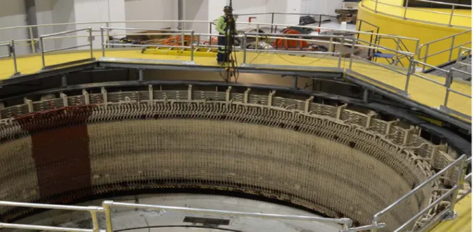
In larger synchronous machines, the stator coils are connected to each other in series and form multiple parallel circuits per phase, which allows the machine to generate significantly more current and thus more power for the same voltage level and coil current rating. These “hydro” units also have a large number of poles, which reduce the machine’s operating speed and stator coil pitch, or the distance between the top half of a stator coil and the bottom half. The top half of a stator coil is the side of the coil which is slotted radially closest to the rotor (or center of the machine), and the bottom half is the side that is slotted radially farthest from the rotor. Figures 2.5 and 2.6, taken from Reclamation site visit pictures, provide an example of the actual rotor and stator of a large synchronous generator, respectively, at the Glen Canyon power plant.

(19)

9

Figure 2.6 Glen Canyon Unit Stator

2.3 Finite Element Analysis

Finite Element Analysis (FEA) is a numerical tool used to approximate solutions to complex systems. To implement FEA, a physical model of the problem is first developed and then overlaid with a mesh grid that divides the model into smaller simpler geometric pieces (triangles, rectangles, etc.) which are called elements. Figure 2.7 shows an example of a mesh grid applied to a synchronous machine model that divides the model into various triangles. The resulting elements of the physical model have a set of approximated difference equations applied to them (i.e. based on Maxwell’s equations). These equations are then solved iteratively (or using other techniques) for each element using either numerical linear algebra, which is preferable for steady state problems, or numerical integration, which is preferable for transient problems. At the end of this process, when the equations for all of the model’s elements are solved for, a global set of equations are obtained that describe the solutions of the entire model.

(20)

10

Figure 2.7 MagNet Mesh Grid Example [10]

The main issues with this or any numerical method involve the convergence of a given model’s solution, the simulation time for the model, and the accuracy of the solution. It is essential that simulations performed on an FEM-based numerical model converge on a solution within a reasonable amount of time, and that the solution accurately describes or predicts the physical properties being analyzed in the model. When developing and analyzing FEM-based models, there is also a tradeoff between the model’s complexity and its accuracy. If an FEM-based model is divided into more elements, it will take longer to obtain a solution, but the solution will be more accurate. On the flip side, a model with less elements can be solved more quickly, but the solution will not be as accurate.

(21)

11 2.3.0 MagNet [10]

MagNet is a FEM-based analysis software, available commercially, which allows the examination of the electromagnetic fields resulting from a given physical model. It allows one to create or import a model whose components each have physical properties including the

component’s magnetic permeability, electric permittivity, and mass density. These properties can be manually specified in a custom material, or a pre-defined material can be applied from

MagNet’s material library. The software solves the given model by first applying a mesh grid that divides a given model into either triangular (2-D modeling) or tetrahedral (3-D modeling) elements. The resulting elements have Maxwell’s equations applied to them, which are then solved using both the Newton Raphson and the Conjugate Gradient methods. Once a solution is obtained, MagNet uses the resulting data (electric and magnetic fields, current densities, etc.) to calculate other parameters for each element, including their forces, currents, and voltages. The solver can perform both steady state and transient simulations, which obtain solutions for multiple time increments instead of just one for steady state simulations.

2.3.0.1 Circuit Window

For each component specifically defined as a coil, MagNet will take the solutions from Maxwell’s equations and calculate the corresponding voltages across the coils and currents through the coils. To analyze the voltages and currents of coils modeled in MagNet, they can be modeled electrically in the software’s circuit window, which allows various components that are connected to the coils but are external to the model. Figure 2.8 shows an example of the circuit window in MagNet.

(22)

12

Figure 2.8 MagNet Circuit Window Example [10]

When a coil is defined in the main window, a corresponding electrical model is created in the circuit window. This model, which appears in a separate sub-window on the left (as shown in Figure 2.8), can be placed in the main window on the right and connected to resistors, inductors, capacitors, voltage or current sources, and other simple electrical components. This feature can be used to drastically reduce the complexity of the entire model while still allowing for a detailed examination of the electrical characteristics of the model’s coils, which reduces the model’s simulation time.

2.3.0.2 Solving in MagNet

When solving a given model, Magnet uses two layers of numerical methods to improve the accuracy of the solution. The Conjugate Gradient method is the inner layer that performs the main calculation, and the Newton Raphson method is the outer layer that refines the solution.

(23)

13

The Conjugate Gradient Method iteratively solves Maxwell’s equations for each element using equations 2.3-2.9 shown below [9]. Once the residual vector r is within a specified

tolerance (called the CG tolerance), the solution is obtained [10].

Ax = b (Linear Matrix System) (2.3)

f(x) = xTAx – 2xTb (2.4) αn = 𝑝𝑛𝑇𝑟𝑛 𝑟𝑛𝑇𝐴𝑟𝑛 (2.5) xn+1 = xn + αnpn (2.6) rn+1 = rn + αnApn (2.7) βn = −𝑝𝑛𝑇𝐴𝑟𝑛+1 𝑝𝑛𝑇𝐴𝑝𝑛 (2.8) pn+1 = rn+1 + βnpn (2.9) Where: x – Solution Vector

A – Positive Definite Matrix (linearized)

b – Given Vector

f(x) – Quadratic Function (Minimized at x)

xT – Transposed Solution Vector p – Direction Vector

(24)

14

r – Residual Vector (Initially set to Ax - b) α – Scalar Multiplier (for Incrementing x)

β – Scaling Multiplier (for Adjusting p)

n – Iteration Number

Once the Conjugate Gradient method obtains a solution, the Newton Raphson method further refines the solution using equations 2.10-2.12 shown below [11]. Similar to the Conjugate Gradient method, once the solution difference ∆x comes within a specified tolerance, the solution is obtained. ∆yn = y – f(xn) (2.10) ∆xn = Jn-1·∆yn (2.11) xn+1 = xn + ∆xn (2.12) Where: x – Solution Vector y – Given Vector f(x) – Given Function Vector

J – Jacobian Matrix n – Iteration Number

(25)

15 CHAPTER 3

APPLICATION TO GLEN CANYON POWER PLANT

3.1 Introduction

There are two hydro units at the Glen Canyon power plant which have had temporary bypass work performed on their stator windings after sustaining significant damage. While performing load tests on unit G2, the Bureau of Reclamation’s (BOR) Diagnostics Team measured the parallel winding currents flowing in this unit at various operating points. A

numerical model was recently developed in Finite Element Method (FEM) modeling software to represent the bypass work performed on the unit. With this model, the operating points measured by the Diagnostics Team were simulated, and the resulting currents calculated in the winding were compared to the corresponding field data to assess the model’s accuracy.

This chapter outlines the history of unit G2 at Glen Canyon power plant from when its winding sustained damaged to when the unit was rewound, details the measurement process and results, describes the inputs and assumptions used to create the numerical model, and shows the simulation results and compares them to the field measurements.

3.2 Unit G2 Damage & Repair History

The stator winding of unit G2 sustained damage on December 1, 2001, as it was being manually brought online [2]. When water from cooling equipment located one floor above the unit leaked into the unit’s air housing deck and into the machine, it caused a ground fault to

(26)

16

occur in the A-phase of the winding. This was detected by the unit’s ground fault relay, which tripped the unit offline before the unit breaker was closed.

During multiple visits to the plant, Reclamation’s Diagnostics Team worked with plant personnel to assess G2’s electrical and physical condition and dried the stator winding by operating the unit into a bolted terminal short. They then located the two stator coils where the fault occurred and electrically isolated them by bypassing the entire parallel circuit that

contained them. The unit was then successfully brought back online on February 20, 2002, and was subsequently operated at reduced capacity until the unit was rewound in November of that year. Figure 3.1 shows a timeline of the events described in this section.

Figure 3.1 Glen Canyon Unit G2 Timeline [8]

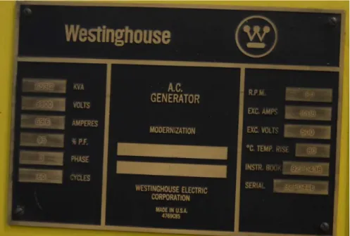
3.3 Unit G2 Nameplate Data

Before the unit was rewound in November 2002, G2’s winding was rated for 165 MVA at 13.8 kV and a lagging power factor of 0.95. After it was rewound, the rating was increased to

(27)

17

174 MVA at the same voltage and power factor. Examples of the full nameplate ratings for each winding (taken from Reclamation site visit pictures) are shown in Figures 3.2 and 3.3 below.

Figure 3.2 Glen Canyon Unit Nameplate – Ratings Prior to 2002 Rewind

(28)

18 3.4 Field Measurements

Prior to unit G2’s rewind, the Diagnostic Team recorded data on the unit’s temporarily repaired winding to examine the effects of electrically bypassing an entire parallel circuit. The measurements consisted of the current flowing in each of the unit’s parallel circuits (excluding the one that was electrically removed), as well as the total current flowing out of each phase of the machine.

3.4.1 Diagnostic Measurement Process

The measurements on G2’s stator winding were recorded while the Diagnostics Team was performing an operating limit test. During the first part of this test, the maximum unit load at unity power factor was determined by incrementally increasing the amount of MW being

generated by the unit and monitoring the resulting currents flowing in each parallel circuit [2]. The maximum load was reached when the maximum circuit current went above the rated current per circuit of the unit, which was 865A. In the second part of this test, the MW output of the unit was lowered to just below the maximum loading limit and the MVAR output was varied so that MVAR flowed into and out of the unit. This allowed the Diagnostics Team to evaluate the effects of MVAR loading on current flow in the winding.

To measure the parallel circuit currents, clamp CTs were connected around each of the remaining 23 jumpers running between the neutral end of the stator circuits and the ring bus along the outside of the winding. An example of this (Also taken from Reclamation site visit pictures) is shown in Figure 3.4. The leads of these clamp CTs were then connected to a given burden board, which produced voltages corresponding to the current flowing into the board. These voltages were related to the input currents by a simple conversion factor determined by the

(29)

19

burden board. Once the output voltage was obtained, the circuit currents were calculated using the burden board and CT ratios.

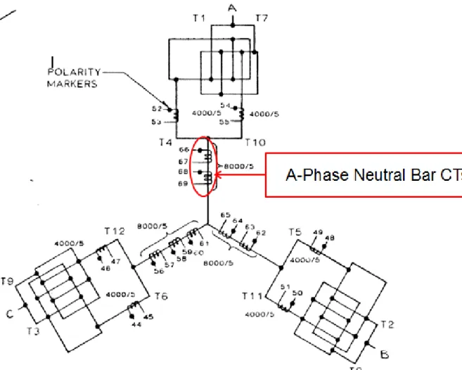
Figure 3.4 Clamp CT Location on Machine Winding

Similarly, the line currents were measured by connecting transducers to the existing metering circuits for the units, which included CTs connected around the neutral bar of each phase of the stator winding. Figure 3.5, which is taken from electrical drawings for unit G2, shows the location of these CTs on the neutral bars. The conversion factor for the transducers and the metering CT ratios were used to calculate the line currents.

(30)

20

Figure 3.5 Glen Canyon Unit G2 – Neutral Bar Drawing with CT Locations

3.4.2 Resulting Data

The measurements made on G2 by the Diagnostics Team were collected at six different operating points, as shown in Figure 3.6. For four of these points, no MVARs were generated or absorbed by the unit (unity power factor) while the maximum loading limit was being

determined; for the other two points, MVARs were generated and absorbed by the unit at a MW loading just below the maximum limit previously determined.

(31)

21

Figure 3.6 Glen Canyon Unit G2 – Measured Operating Points

The following tables detail the resulting currents measured from G2. Table 3.1 shows the field and line currents measured for each operating point. Tables 3.2, 3.3, and 3.4 show the parallel circuit currents for phases A, B, and C, respectively, as well as the percentage of total line current each circuit generates. Note that there are no measurements for circuit A5, as this was the circuit electrically removed from G2’s winding. There are also no measurements for circuit B7, since the clamp CT placed on this circuit’s jumper failed during testing.

0 20 40 60 80 100 120 140 160 180 200 -200 -150 -100 -50 0 50 100 150 200

Glen Canyon Unit 2 - Measured Operating Points

Active Power (MW) R eac ti v e P ow er ( M V A R )

Stator Limit (Undamaged Unit) Stator Limit (Damaged Unit) Measured Operating Points

(32)

22

Table 3.1 Glen Canyon Unit G2 – Measured Field Current and Phase Currents

Glen Canyon Unit 2 - Measured Field Current and Phase Currents MW MVAR If (A) Ia (A) Ib (A) Ic (A) Average Current (A) 39.4 -1.3 466 1552 1648 1776 1659 100 0 580 4032 4240 4336 4203 130 0 650 5216 5536 5600 5451 135 0 662 5488 5760 5800 5683 124.5 29 772 5088 5312 5456 5285 125.8 -32.6 500 5264 5584 5696 5515

Table 3.2 Glen Canyon Unit G2 – Measured A-Phase Circuit Currents

Glen Canyon Unit 2 - Measured A-Phase Circuit Currents

Unit Loading T4-26 T10-71 T4-116 T10-161

MW MVAR A1 (A) % of Ia A2 (A) % of Ia A3 (A) % of Ia A4 (A) % of Ia

39.4 -1.3 230 14.80% 168 10.80% 212 13.70% 211 13.60% 100 0 582 14.40% 570 14.10% 564 14.00% 565 14.00% 130 0 753 14.40% 740 14.20% 732 14.00% 730 14.00% 135 0 785 14.30% 774 14.10% 768 14.00% 765 13.90% 124.5 29 735 14.40% 721 14.20% 715 14.10% 713 14.00% 125.8 -32.6 759 14.40% 740 14.10% 734 13.90% 740 14.10% Unit Loading T4-206 T10-251 T4-296 T10-341

MW MVAR *A5 (A) % of Ia A6 (A) % of Ia A7 (A) % of Ia A8 (A) % of Ia

39.4 -1.3 N/A N/A 236 15.20% 230 14.80% 222 14.30% 100 0 N/A N/A 608 15.10% 584 14.50% 575 14.30% 130 0 N/A N/A 788 15.10% 756 14.50% 747 14.30% 135 0 N/A N/A 824 15.00% 790 14.40% 780 14.20% 124.5 29 N/A N/A 768 15.10% 735 14.40% 727 14.30% 125.8 -32.6 N/A N/A 792 15.00% 765 14.50% 756 14.40%

(33)

23

Table 3.3 Glen Canyon Unit G2 – Measured B-Phase Circuit Currents

Glen Canyon Unit G2 - Measured B-Phase Circuit Currents

MW MVAR B1 (A) % of Ib B2 (A) % of Ib B3 (A) % of Ib B4 (A) % of Ib

MW MVAR B5 (A) % of Ib B6 (A) % of Ib **B7(A) % of Ib B8 (A) % of Ib

39.4 -1.3 242 14.70% 214 13.00% N/A N/A 202 12.30% 100 0 624 14.70% 538 12.70% N/A N/A 517 12.20% 130 0 805 14.50% 692 12.50% N/A N/A 667 12.00% 135 0 843 14.60% 723 12.60% N/A N/A 696 12.10% 124.5 29 777 14.60% 667 12.60% N/A N/A 641 12.10% 125.8 -32.6 817 14.60% 705 12.60% N/A N/A 681 12.20%

** Clamp-on CT failed, no data recorded

Table 3.4 Glen Canyon Unit G2 – Measured C-Phase Circuit Currents

Glen Canyon Unit G2 - Measured C-Phase Circuit Currents

MW MVAR C1 (A) % of Ic C2 (A) % of Ic C3 (A) % of Ic C4 (A) % of Ic

MW MVAR C5 (A) % of Ic C6 (A) % of Ic C7 (A) % of Ic C8 (A) % of Ic

39.4 -1.3 258 14.50% 226 12.70% 221 12.40% 217 12.20% 100 0 634 14.60% 538 12.40% 525 12.10% 524 12.10% 130 0 822 14.70% 691 12.30% 678 12.10% 675 12.10% 135 0 850 14.70% 715 12.30% 697 12.00% 696 12.00% 124.5 29 802 14.70% 672 12.30% 657 12.00% 654 12.00% 125.8 -32.6 828 14.50% 704 12.40% 695 12.20% 686 12.00%

(34)

24

Tables 3.5, 3.6, and 3.7 similarly show the parallel circuit currents for phases A, B, and C, respectively; they also include a comparison to the expected currents in an equivalent undamaged machine using a per-unit current calculation. This calculation is performed using equations 3.1 and 3.2, where 𝑉_𝑡 represents the rated terminal voltage of the machine and ‘# of circuits’ represents the number of parallel circuits per phase in the machine winding.

Ibase = √𝑀𝑊2+ 𝑀𝑉𝐴𝑅2

√3∗𝑉𝑡∗(# 𝑜𝑓 𝑐𝑖𝑟𝑐𝑢𝑖𝑡𝑠) (3.1)

Ipu = 𝐼𝑚𝑒𝑎𝑠𝑢𝑟𝑒𝑑

𝐼𝑏𝑎𝑠𝑒 (3.2)

Table 3.5 Glen Canyon Unit G2 – Measured A-Phase Per-Unit Circuit Currents

Glen Canyon Unit G2 - Measured A-Phase Per-Unit Circuit Currents

MW MVAR Ibase (A) A1 (A) P.U. A2 (A) P.U. A3 (A) P.U. A4 (A) P.U.

39.4 -1.3 206.15 230 1.12 168 0.81 212 1.03 211 1.02 100 0 522.96 582 1.11 570 1.09 564 1.08 565 1.08 130 0 679.85 753 1.11 740 1.09 732 1.08 730 1.07 135 0 706.00 785 1.11 774 1.10 768 1.09 765 1.08 124.5 29 668.50 735 1.10 721 1.08 715 1.07 713 1.07 125.8 -32.6 679.64 759 1.12 740 1.09 734 1.08 740 1.09 Unit Loading T4-206 T10-251 T4-296 T10-341

MW MVAR Ibase (A) *A5

(A) P.U. A6 (A) P.U. A7 (A) P.U. A8 (A) P.U.

39.4 -1.3 206.15 N/A N/A 236 1.14 230 1.12 222 1.08 100 0 522.96 N/A N/A 608 1.16 584 1.12 575 1.10 130 0 679.85 N/A N/A 788 1.16 756 1.11 747 1.10 135 0 706.00 N/A N/A 824 1.17 790 1.12 780 1.10 124.5 29 668.50 N/A N/A 768 1.15 735 1.10 727 1.09 125.8 -32.6 679.64 N/A N/A 792 1.17 765 1.13 756 1.11

(35)

25

Table 3.6 Glen Canyon Unit G2 – Measured B-Phase Per-Unit Circuit Currents

Glen Canyon Unit G2 - Measured B-Phase Per-Unit Circuit Currents

MW MVAR Ibase (A) B1 (A) P.U. B2 (A) P.U. B3 (A) P.U. B4 (A) P.U.

MW MVAR Ibase (A) B5 (A) P.U. B6 (A) P.U. **B7

(A) P.U. B8 (A) P.U.

39.4 -1.3 206.15 242 1.17 214 1.04 N/A N/A 202 0.98 100 0 522.96 624 1.19 538 1.03 N/A N/A 517 0.99 130 0 679.85 805 1.18 692 1.02 N/A N/A 667 0.98 135 0 706.00 843 1.19 723 1.02 N/A N/A 696 0.99 124.5 29 668.50 777 1.16 667 1.00 N/A N/A 641 0.96 125.8 -32.6 679.64 817 1.20 705 1.04 N/A N/A 681 1.00

** Clamp-on CT failed, no data recorded

Table 3.7 Glen Canyon Unit G2 – Measured C-Phase Per-Unit Circuit Currents

Glen Canyon Unit G2 - Measured C-Phase Per-Unit Circuit Currents

MW MVAR Ibase (A) C1 (A) P.U. C2 (A) P.U. C3 (A) P.U. C4 (A) P.U.

MW MVAR Ibase (A) C5 (A) P.U. C6 (A) P.U. C7 (A) P.U. C8 (A) P.U.

39.4 -1.3 206.15 258 1.25 226 1.10 221 1.07 217 1.05 100 0 522.96 634 1.21 538 1.03 525 1.00 524 1.00 130 0 679.85 822 1.21 691 1.02 678 1.00 675 0.99 135 0 706.00 850 1.20 715 1.01 697 0.99 696 0.99 124.5 29 668.50 802 1.20 672 1.01 657 0.98 654 0.98 125.8 -32.6 679.64 828 1.22 704 1.04 695 1.02 686 1.01

(36)

26

The maximum load limit from the measurements shown above was determined to be 135 MVA, or roughly 82% of the rated operating limit for G2 prior to sustaining damage. Overall, this meant an 18% reduction in loading from the rated operating limit for G2. The reduction in loading recommended based on EPRI report EL-4983 [1] was only half of this (9%), which would have put the loading limit at 91% of the rated operating limit.

From these measurements, the effect of removing an entire parallel circuit from G2’s stator winding can be seen. Since circuit A5 was removed, the magnetic flux from the rotor induced higher voltages (and thus higher currents) in the corresponding circuits B5 and C5. The highest parallel circuit current measured in G2’s stator winding at the maximum load limit was 850A in circuit C5, which is just below the rated current per circuit, 865A. As shown by Table 3.7, this value was 20% higher than what the current would have been in a similar undamaged winding.

3.5 Unit G2 Model

A 2-D symmetrical model, shown in Figure 3.7, was created for unit 2 at Glen Canyon using the FEM-based software, MagNet [10]. This model was developed primarily using drawings and machine data provided by the U.S. Bureau of Reclamation (USBR), which included nameplate ratings, physical dimensions, and winding coil connections. The numerical model was used to run simulations of both the damaged winding from 2002 and the current undamaged winding, and the results were compared to the previously mentioned field data to assess the accuracy of the model.

(37)

27

(38)

28 3.5.1 Model Inputs & Assumptions

The general information that was used to create the 2-D synchronous machine model in MagNet included information on the number of poles and stator coils, the number of turns per coil (rotor and stator coils), the stator coil pitch, the air gap thickness, and the depth of the core material (which was used to define the depth of the entire model). These inputs are listed in Table 3.8.

Table 3.8 Glen Canyon Unit G2 – General Information

General Parameters Value

Number of Poles 48

Number of Rotor Coil Turns (per pole) 33

Number of Stator Coils 360

Number of Stator Coil Turns (per coil) 3

Stator Coil Pitch 1 to 8

Air Gap Thickness (inches) 0.58

Model Depth (inches; based on core depth) 83.5

Number of Stator Circuits (per phase) 8

The physical dimensions used to develop the model for G2 were divided among those for the stator, those for the rotor, and those for the damper bars. Table 3.9 shows these dimensions, which were used to create the outlines for the rotor core, poles and coils, the stator core and coils, and the damper bars.

Once the model outline was finished, each of the components was created using the model depth specified in Table 3.8. The damper bars, rotor coils, and stator coils were modeled as solid pieces (including insulation) using the pre-defined model material ‘Copper: 101% IACS (ETP)’ from MagNet’s material library. Both cores and all 48 poles were modeled with user defined materials. The magnetic permeability and loss data for these materials were referenced

(39)

29

from a similar CEATI study [3], whose report is titled Operation of Hydro Generators with Bypassed Stator Coils. The mass density for these materials was provided by USBR.

Table 3.9 Glen Canyon Unit G2 – Physical Dimensions

Stator Parameters Value (inches)

Stator Inner Radius 155

Stator Outer Radius 168.875

Wedge Offset 0.015

Wedge Length (radial) 0.188

Wedge Width 0.1085

Stator Coil Length 3.2185

Stator Coil Width 0.907

Rotor Parameters Value (inches)

Core Inner Radius 124.5

Core Outer Radius (w/out poles) 139.045

Core + Poles Outer Radius 154.42

Coil Length 11.022

Coil Width 2.085

Pole Length w/out Tooth 13

Tooth Inner Width 10.75

Tooth Outer Width 14.75

Pole Face Radius - Center 42.6473

Pole Face Radius - Side 0.9884

Damper Winding Parameters Value (inches)

Damper Bar Diameter 0.75

Damper Bar Radius 0.375

Pole Face Edge (Center) to Center Bar 0.5857

Pole Face Edge (Center) to 1 Bar out 0.6589

Pole Face Edge (Center) to 2 Bars Out 1.025

Center Bar to 1 Bar out 2.9286

(40)

30

3.5.2 Model Inputs and Assumptions – Circuit Window

To model the coil connections for the field winding, stator winding, and damper bars, the coil components were grouped together and defined as coils which created corresponding

electrical components for them in the circuit window. An example of this is shown in Figure 3.8.

Figure 3.8 Coil Components Example (Taken from Unit G2 Model)

Since the field winding was not altered during the bypass work, all 48 coils were grouped together to form a single component in the circuit window, which was connected to an

independent current source that supplied the DC field current. This current was updated with the measured field currents from Table 3.1. The damper bar components in the circuit window were all shorted together on both ends, just like the actual damper bars on unit G2. The resulting field and damper windings are shown in Figures 3.9 and 3.10, respectively.

(41)

31

Figure 3.9 Glen Canyon Unit G2 Circuit Window - Field Winding

(42)

32

The stator coils for G2 are connected together in alternating groups of two and three coils in series going around the stator. Each stator circuit consists of six coil groups, or fifteen

individual coils, and there are eight circuits paralleled together per phase (24 circuits total). Since the end windings were not modeled in the main window, they were modeled in the circuit

window as a single resistor and inductor for each parallel circuit, which represented the total resistance and leakage reactance of all 15 coils per circuit lumped together. The values used for the end winding resistance and leakage reactance were referenced from the CEATI study

mentioned in section 3.5.1. To represent the loading of the unit, a simple three-phase impedance was connected to each phase of the stator winding. The value of this impedance was changed with loading, and was calculated using equations 3.3-3.6. Figure 3.11 shows a portion of the Reclamation drawing referenced for the winding connections, and Figure 3.12 shows the resulting circuit of one phase (including the load impedance). To model the bypass work performed on G2, circuit A5 was disconnected from the rest of the A-phase circuit; the circuit removed is circled in Figure 3.12.

Zload = 𝑉𝑡2 √𝑀𝑊2_{+ 𝑀𝑉𝐴𝑅}2 (3.3) Rload = Zload*PF (3.4) Lload = �𝑍𝑙𝑜𝑎𝑑 2_{− 𝑅} 𝑙𝑜𝑎𝑑2 120∗𝜋 (3.5) Cload = 120∗𝜋 �𝑍𝑙𝑜𝑎𝑑2_{− 𝑅𝑙𝑜𝑎𝑑}2 (3.6) Where: Vt – Terminal Voltage

(43)

33

Zload – Load Impedance Rload – Load Resistance

PF – Power Factor

Lload – Load Inductance (Lagging PF Load Only)

Cload – Load Capacitance (Leading PF Load Only)

(44)

34

Figure 3.12 Glen Canyon Unit G2 Circuit Window – Stator Winding Including Load Impedance

3.6 Simulation Results

Using the model developed for Glen Canyon Unit G2, transient simulations were

performed at seven different operating points: one at the rated conditions of the existing unit, and six at the operating points described in section 3.4.2.The solver parameters used for these

simulations are detailed in Table 3.10.

Table 3.10 Glen Canyon Unit G2 – Solver Parameters

Parameter Value

Maximum Newton Iterations 50

Newton Tolerance 1%

Polynomial Order 2

CG Tolerance 0.01%

Transient Simulation Stop Time 450ms Transient Simulation Time Step 1ms

(45)

35

To assess the accuracy of the simulated voltages and currents, the simulation results were compared to the machine ratings and the field measurements in the following tables. Since MagNet produces time domain currents and voltages, the RMS of these values were calculated using MATLAB code (given in Appendix A). The simulated voltages were each expressed in kV and as a per unit value of the machine’s rated phase voltage. For the phase and parallel circuit currents, the percentage difference between the simulated and measured currents were displayed below the simulated and measured values. The percentage difference for each simulated current was calculated using equation 3.7. Tables 3.11-3.17 cover the phase voltages and line currents calculated for each simulation. Tables 3.18-3.23 cover the parallel circuit currents calculated for each simulation.

Margin of Error = (𝐼𝑠𝑖𝑚𝑢𝑙𝑎𝑡𝑒𝑑

𝐼𝑚𝑒𝑎𝑠𝑢𝑟𝑒𝑑 - 1)*100% (3.7) Table 3.11 Unit G2 Model Simulation Results (Phase Voltages & Currents) – Existing Ratings

Glen Canyon Undamaged Model - 100% Load, PF = 0.95 Lagging

S (MVA) 173.7

P (MW) 165.0

Q (MVAR) 54.2

Terminal Voltage (kV) 13.8

Field Current (A) 1040

Simulation Results

Phase A B C

Voltage

Simulated Phase Voltage (kV) 8.31 8.29 8.31 Per Unit Voltage (p.u.) 1.04 1.04 1.04

Current

Simulated Current (A) 7514 7512 7511

Measured Current (A) 7267 7267 7267

Margin of Error (%) 3.40 3.37 3.36

(46)

36

Table 3.12 Unit G2 Simulation Results (Phase Voltages & Currents) – 23% Load, PF = 1.0

Glen Canyon Unit 2 - 23% Load, PF = 1.0 (Unity; Modeled with leading PF due to small amount of MVAR absorbed)

S (MVA) 39.4

P (MW) 39.4

Q (MVAR) -1.3

Simulation Results

Phase A B C

Voltage

Current

Margin of Error (%) 0.52 -5.64 -11.71

*All results are rms, symmetrical

Glen Canyon Unit 2 - 58% Load, PF = 1.0 (Unity)

S (MVA) 100.0

P (MW) 100.0

Q (MVAR) 0.0

Simulation Results

Phase A B C

Voltage

Current

Margin of Error (%) 1.74 -3.68 -4.84

(47)

37

S (MVA) 130.0

P (MW) 130.0

Q (MVAR) 0.0

Simulation Results

Phase A B C

Voltage

Current

Margin of Error (%) 3.59 -2.93 -2.88

S (MVA) 135.0

P (MW) 135.0

Q (MVAR) 0.0

Simulation Results

Phase A B C

Voltage

Current

Margin of Error (%) 2.33 -3.04 -2.50

(48)

38

Table 3.16 Unit G2 Simulation Results (Phase Voltages & Currents) – 74% Load, PF = 0.97 Lag

Glen Canyon Unit 2 - 74% Load, PF = 0.97 Lagging

S (MVA) 127.8

P (MW) 124.5

Q (MVAR) 29.0

Simulation Results

Phase A B C

Voltage

Current

Margin of Error (%) 6.03 1.34 -0.31

Table 3.17 Unit G2 Simulation Results (Phase Voltages & Currents) – 58% Load, PF = 0.97Lead

Glen Canyon Unit 2 - 75% Load, PF = 0.97 Leading

S (MVA) 130

P (MW) 125.8

Q (MVAR) -32.6

Simulation Results

Phase A B C

Voltage

Current

Margin of Error (%) -3.04 -9.29 -9.88

(49)

39

Table 3.18 Unit G2 Simulation Results (Parallel Circuit Currents) – 23% Load, PF – 1.0

Glen Canyon Unit 2 - 23% Load, PF = 1.0 (Unity; Modeled with leading PF due to small amount of MVAR absorbed)

A-Phase A1 A2 A3 A4 A5 A6 A7 A8 Simulated Current (A) 221.3 220.8 220.5 221.4 0 229.3 224.3 222.7 Measured Current (A) 230 168 212 211 0 236 230 222 Margin of Error (%) -3.78 31.43 4.01 4.93 N/A -2.84 -2.48 0.32 B-Phase B1 B2 B3 B4 B5 B6 B7 B8 Simulated Current (A) 194.2 193.6 193 200 220 200.7 197.1 195.4 Measured Current (A) 209 186 179 200 242 214 N/A 202 Margin of Error (%) -7.08 4.09 7.82 0.00 -9.09 -6.21 N/A -3.27 C-Phase C1 C2 C3 C4 C5 C6 C7 C8 Simulated Current (A) 193.6 192.6 192.7 209.3 217.3 197.2 195.9 194.1 Measured Current (A) 214 205 201 233 258 226 221 217 Margin of Error (%) -9.53 -6.05 -4.13 -10.17 -15.78 -12.74 -11.36 -10.55 *All results are rms, symmetrical

Table 3.19 Unit G2 Simulation Results (Parallel Circuit Currents) – 58% Load, PF = 1.0

A-Phase A1 A2 A3 A4 A5 A6 A7 A8 Simulated Current (A) 584.8 583.2 581.5 577.4 0 599.5 589 586.9 Measured Current (A) 582 570 564 565 0 608 584 575 Margin of Error (%) 0.48 2.32 3.10 2.19 N/A -1.40 0.86 2.07 B-Phase B1 B2 B3 B4 B5 B6 B7 B8 Simulated Current (A) 499.2 497.2 494.7 522.9 582.9 509.1 502.7 501.1 Measured Current (A) 532 500 490 528 624 538 N/A 517 Margin of Error (%) -6.17 -0.56 0.96 -0.97 -6.59 -5.37 N/A -3.08 C-Phase C1 C2 C3 C4 C5 C6 C7 C8 Simulated Current (A) 513.4 510.3 508.6 576.9 593.8 517.1 516.5 514 Measured Current (A) 518 515 515 585 634 538 525 524 Margin of Error (%) -0.89 -0.91 -1.24 -1.38 -6.34 -3.88 -1.62 -1.91 *All results are rms, symmetrical

(50)

40

A-Phase A1 A2 A3 A4 A5 A6 A7 A8 Simulated Current (A) 767.1 766.1 765.7 761.4 0 797.3 775.6 769.9 Measured Current (A) 753 740 732 730 0 788 756 747 Margin of Error (%) 1.87 3.53 4.60 4.30 N/A 1.18 2.59 3.07 B-Phase B1 B2 B3 B4 B5 B6 B7 B8 Simulated Current (A) 651.1 650 648 680.4 764.8 670 657.2 653.4 Measured Current (A) 692 652 642 681 805 692 N/A 667 Margin of Error (%) -5.91 -0.31 0.93 -0.09 -4.99 -3.18 N/A -2.04 C-Phase C1 C2 C3 C4 C5 C6 C7 C8 Simulated Current (A) 675.3 673.4 671.9 761.9 793.6 685.8 680.4 675.6 Measured Current (A) 672 667 672 756 822 691 678 675 Margin of Error (%) 0.49 0.96 -0.01 0.78 -3.45 -0.75 0.35 0.09 *All results are rms, symmetrical

A-Phase A1 A2 A3 A4 A5 A6 A7 A8 Simulated Current (A) 797 796 795.7 791.3 0 829.6 806.3 800 Measured Current (A) 785 774 768 765 0 824 790 780 Margin of Error (%) 1.53 2.84 3.61 3.44 N/A 0.68 2.06 2.56 B-Phase B1 B2 B3 B4 B5 B6 B7 B8 Simulated Current (A) 675.9 674.8 672.8 705.9 794.2 696.3 682.6 678.4 Measured Current (A) 698 684 674 715 843 723 N/A 696 Margin of Error (%) -3.17 -1.35 -0.18 -1.27 -5.79 -3.69 N/A -2.53 C-Phase C1 C2 C3 C4 C5 C6 C7 C8 Simulated Current (A) 701.8 699.9 698.6 792.4 826.8 713.6 707.4 702.3 Measured Current (A) 695 690 692 780 850 715 697 696 Margin of Error (%) 0.98 1.43 0.95 1.59 -2.73 -0.20 1.49 0.91 *All results are rms, symmetrical

(51)

41

Table 3.22 Unit G2 Simulation Results (Parallel Circuit Currents) – 74% Load, PF – 0.97 Lag

Glen Canyon Unit 2 - 74% Load, PF = 0.97 Lagging

A-Phase A1 A2 A3 A4 A5 A6 A7 A8 Simulated Current (A) 766.1 765.1 764.8 759.1 0 796.7 774.6 768.6 Measured Current (A) 735 721 715 713 0 768 735 727 Margin of Error (%) 4.23 6.12 6.97 6.47 N/A 3.74 5.39 5.72 B-Phase B1 B2 B3 B4 B5 B6 B7 B8 Simulated Current (A) 644.9 643.8 641.9 672.7 755.1 664.2 650.7 647.1 Measured Current (A) 642 632 627 657 777 667 N/A 641 Margin of Error (%) 0.45 1.87 2.38 2.39 -2.82 -0.42 N/A 0.95 C-Phase C1 C2 C3 C4 C5 C6 C7 C8 Simulated Current (A) 676.9 675 674 765.7 801.8 687.9 682 677.2 Measured Current (A) 656 650 652 737 802 672 657 654 Margin of Error (%) 3.19 3.85 3.37 3.89 -0.02 2.37 3.81 3.55 *All results are rms, symmetrical

Table 3.23 Unit G2 Simulation Results (Parallel Circuit Currents) – 75% Load, PF – 0.97 Lead

Glen Canyon Unit 2 - 75% Load, PF = 0.97 Leading

A-Phase A1 A2 A3 A4 A5 A6 A7 A8

Simulated Current (A) 725.1 723.7 722.7 721 0 751.7 732.1 727.8

Measured Current (A) 759 740 734 740 0 792 765 756

Margin of Error (%) -4.47 -2.20 -1.54 -2.57 N/A -5.09 -4.30 -3.73

B-Phase B1 B2 B3 B4 B5 B6 B7 B8

Simulated Current (A) 623.3 621.9 619.4 649.5 719.9 640.4 628.8 625.7

Measured Current (A) 675 660 756 695 817 705 N/A 681

Margin of Error (%) -7.66 -5.77 -18.07 -6.55 -11.88 -9.16 N/A -8.12

C-Phase C1 C2 C3 C4 C5 C6 C7 C8

Simulated Current (A) 635.7 633.6 631.5 707.9 731.8 643.3 640 636.5

Measured Current (A) 678 678 680 765 828 704 695 686

Margin of Error (%) -6.24 -6.55 -7.13 -7.46 -11.62 -8.62 -7.91 -7.22

(52)

42

While the simulation performed at a loading of 23% (Tables 3.12 & 3.18) was effectively a unity power factor operating point, there was a small amount of MVAR absorbed by the unit when the corresponding field measurements were made, and it was thus modeled with a leading power factor to account for this. The resulting currents from this simulation also appear to vary greatly from the corresponding measured currents, with the greatest margin of error being calculated at over 30%. However, since the loading per circuit was measured at lower levels around 200A, the deviation between simulated and measured current levels is exaggerated. A difference in magnitude of 60A at this loading would result in a margin of error of about 30%, whereas the same difference at a loading of roughly 700A per circuit would result in a less than 10% margin of error.

3.7 Conclusion

An FEM-based model was developed for unit G2 at the Glen Canyon power plant to assess the accuracy of numerical modeling in determining new operating points for synchronous machines with bypassed coils. The simulations performed at the operating points with either a unity power factor (excluding the low loading operating point) or a lagging power factor produced currents that were within a 7% margin of error. The simulations performed at the operating points with a leading power factor produced currents that were less accurate, with the worst case margin of error at roughly 18%. Overall, while the majority of simulations performed for this unit produced results within an acceptable margin of error, the inputs and assumptions could be refined to obtain more accurate results for operating points with a leading power factor. This may include modifying the mesh grid to create more elements along the unit’s air gap or within the stator coils, or updating the passive load impedances in MagNet’s circuit window to more accurately represent the current flow in the stator winding.

(53)

43 CHAPTER 4

CONCLUSIONS & FUTURE WORK 4.1 Conclusions

This thesis examined the viability of determining the operating limits of synchronous machines with temporarily bypassed coils using finite element method based software. A study was performed on a synchronous machine with bypassed coils at the Glen Canyon power plant, in which the operation of unit G2 was modeled and the resulting stator winding current data was compared to field measurement data to assess the model’s accuracy.

The model developed for unit G2 accurately simulated the majority of the data points measured at Glen Canyon, with all but one simulation producing stator winding currents within 7% of the corresponding measured values. These results validate the model as an effective means of examining the stator winding currents produced by a synchronous machine with bypassed coils. However, refining the inputs and assumptions that were used to develop the model may yield more accurate results, particularly when simulating an operating point with a leading power factor.

4.2 Thesis Contribution

In order to help ensure the reliability of synchronous machines, the adequate evaluation of their performance after sustaining damage and having temporary repairs performed on them is essential. A more accurate assessment of the performance capabilities of these machines further guarantees their reliability and value to the public.

(54)

44 The main contributions of this thesis include:

1. Examining a more accurate method for determining machine operating limits through numerical modeling in Finite Element Method-based software.

2. Developing a machine modeling process which can be used to investigate other issues relevant to the operation of synchronous machines, including:

a. Normal steady-state operation of machines

b. Various fault scenarios within machine windings – single turn faults in coils, etc. c. Performing/Validating Relay Coordination

4.3 Future Work

With the work discussed in this thesis, there are a number of projects that will be undertaken in the future moving forward:

• Further refine the inputs and assumptions for the existing model for unit G2 at Glen Canyon to potentially improve its accuracy further in modeling current flows in the stator winding.

• Perform additional simulations using G2 model to examine: [1] single turn faults in rotor or stator coils.

[2] alternative repair methods (i.e., only removing damaged coils instead of entire circuit)

[3] existing protective relay settings and how it affects the protection of the machine.

• Develop numerical models for units similar to G2 (bypassed coils) that are overseen by the Bureau of Reclamation and perform similar studies with them.

(55)

45

• Develop visual basic code to be implemented within MagNet to drastically reduce model creation time.

(56)

46 REFERENCES

[1] Brightly, W.B., Brown, C.A., Kelch, E.J., Rhudy, R.G., and Snively, H.D., Synchronous Machine Operation with Cutout Coils, EPRI EL-4983, 1987.

[2] Dehaan, J., Research Field Test Results for Glen Canyon Unit 2 (Draft), U.S. Bureau of Reclamation, Denver 2003

[3] Elez, A. et al., Operation of Hydro Generators with Bypassed Stator Coils, Center for Energy Advancement through Technological Innovation (CEATI). Montreal 2014 [4] Glen Canyon Operating Hours_2014, Retrieved from

http://intra.usbr.gov/itops/information-services/apps/POMTS [5] Grand Coulee Operating Hours_2014, Retrieved from

http://intra.usbr.gov/itops/information-services/apps/POMTS

[6] Inan, A., and Inan, U., Engineering Electromagnetics, Addison Wesley Longman, Inc., California 1999

[7] Pyrhonen, J., Jokinen, T., and Hrabovcova, V. Design of Rotating Electrical Machines, 2nd Edition, John Wiley and Sons, West Sussex, United Kingdom 2014. [8] Rux, L., Dehaan, J., and Atwater, P., Glen Canyon Powerplant Unit 2 Stator Winding

Insulation Failure Diagnostics and Temporary Repair (Draft), U.S. Bureau of Reclamation, Denver 2002

[9] Silvester, P., and Ferrari, R., Finite elements for electrical engineers, 3rd Edition, Cambridge University Press, New York 1996

[10] MagNet. Version 7.5.0.121. Computer software. Infolytica Corporation, 1998. Windows 7.

[11] Glover, J., Overbye, T., and Sarma, M., Power System Analysis and Design, 5th Edition, Cengage Learning, Stamford, Connecticut 2008

(57)

47 APPENDIX

MATLAB CODE USED TO CALCULATE RMS OF SIMULATED MACHINE VOLTAGES & CURRENTS

% Moshe Redmon

% MagNet Results - Analysis % 8-1-2014 %--- clear all close all clc %--- % Simulation Results

disp(['Open Simulation Data File']);

[NUMI,TXTI,RAWI] = xlsread('GLENC_3BP - 1.0 PF (39.4MW) MATLAB data.xlsx',1); [NUMV,TXTV,RAWV] = xlsread('GLENC_3BP - 1.0 PF (39.4MW) MATLAB data.xlsx',2); disp(['Simulation Data File Successfully Opened']);

% Simulation Data for Machine Currents & Voltages Ia = NUMI(34:51,9:16)'; Iat = NUMI(34:51,17)'; Va = NUMV(34:51,3)' + NUMV(34:51,4)'; Ib = [NUMI(34:51,18:21),NUMI(34:51,23:26)]'; Ibt = NUMI(34:51,22)'; Vb = NUMV(34:51,5)' + NUMV(34:51,6)'; Ic = NUMI(34:51,27:34)'; Ict = NUMI(34:51,35)'; Vc = NUMV(34:51,7)' + NUMV(34:51,8)'; time = [0:(length(Ia(1,:))-1)]; time2 = [0:0.01:100/6]; % Curve-Fitting Parameters Ni = 11; Pia = zeros(length(time2),(Ni+1),8); Pib = zeros(length(time2),(Ni+1),8); Pic = zeros(length(time2),(Ni+1),8);

(58)

48 for ii = 1:8 Pia(:,:,ii) = ones(length(time2),1)*polyfit(time,Ia(ii,:),Ni); Pib(:,:,ii) = ones(length(time2),1)*polyfit(time,Ib(ii,:),Ni); Pic(:,:,ii) = ones(length(time2),1)*polyfit(time,Ic(ii,:),Ni); end Piat = ones(length(time2),1)*polyfit(time,Iat,Ni); Pibt = ones(length(time2),1)*polyfit(time,Ibt,Ni); Pict = ones(length(time2),1)*polyfit(time,Ict,Ni); Nv = 9; Pva = ones(length(time2),1)*polyfit(time,Va,Nv); Pvb = ones(length(time2),1)*polyfit(time,Vb,Nv); Pvc = ones(length(time2),1)*polyfit(time,Vc,Nv);

% Resulting Current & Voltage Waveforms Ia2 = zeros(8,length(time2)); Ib2 = zeros(8,length(time2)); Ic2 = zeros(8,length(time2)); Iat2 = zeros(1,length(time2)); Ibt2 = zeros(1,length(time2)); Ict2 = zeros(1,length(time2)); Va2 = zeros(1,length(time2)); Vb2 = zeros(1,length(time2)); Vc2 = zeros(1,length(time2)); for ii = 1:Ni+1 for jj = 1:8

Ia2(jj,:) = Ia2(jj,:) + Pia(:,ii,jj)'.*time2.^(Ni+1-ii); Ib2(jj,:) = Ib2(jj,:) + Pib(:,ii,jj)'.*time2.^(Ni+1-ii); Ic2(jj,:) = Ic2(jj,:) + Pic(:,ii,jj)'.*time2.^(Ni+1-ii); end

Iat2 = Iat2 + Piat(:,ii)'.*time2.^(Ni+1-ii); Ibt2 = Ibt2 + Pibt(:,ii)'.*time2.^(Ni+1-ii); Ict2 = Ict2 + Pict(:,ii)'.*time2.^(Ni+1-ii); end

for ii = 1:Nv+1

Va2 = Va2 + Pva(:,ii)'.*time2.^(Nv+1-ii); Vb2 = Vb2 + Pvb(:,ii)'.*time2.^(Nv+1-ii); Vc2 = Vc2 + Pvc(:,ii)'.*time2.^(Nv+1-ii); end

(59)

49

% RMS Currents & Voltages Iarms = zeros(9,1); Ibrms = zeros(9,1); Icrms = zeros(9,1); Vrms = zeros(3,1); Iarms(1:8) = sqrt(sum(Ia2(1:8,:)'.^2)/length(Ia2(1,:))); Iarms(9) = sqrt(sum(Iat2.^(2))/length(Iat2)); Vrms(1) = sqrt(sum(Va2.^2)/length(Va2)); Ibrms(1:8) = sqrt(sum(Ib(1:8,:)'.^2)/length(Ib(1,:))); Ibrms(9) = sqrt(sum(Ibt2.^(2))/length(Ibt2)); Vrms(2) = sqrt(sum(Vb2.^2)/length(Vb2)); Icrms(1:8) = sqrt(sum(Ic(1:8,:)'.^2)/length(Ic(1,:))); Icrms(9) = sqrt(sum(Ict2.^(2))/length(Ict2)); Vrms(3) = sqrt(sum(Vc2.^2)/length(Vc2));