Adaptive Sub band GSC Beam forming using Linear Microphone-Array for Noise Reduction/Speech Enhancement.

Master’s Thesis:

Electrical Engineering with Emphasis on Signal Processing

Adaptive Sub band GSC Beam forming using Linear

Microphone-Array for Noise Reduction/Speech

Enhancement.

Mamun Ahmed

This thesis is presented as part of Degree of

Master of Science in Electrical Engineering with emphasis on Signal Processing

Blekinge Institute of Technology

February 2012

Blekinge Institute of Technology School of Engineering

Department of Signal Processing Supervisor: Dr. Nedelko Grbic Examiner: Dr. Benny Sällberg

Contact Information

Mamun Ahmed

E-mail: maah09@student.bth.se, mamuncse99cuet@yahoo.com

Supervisor:

Dr. Nedelko Grbic Department of Signal Processing Blekinge Institute of Technology SE-371 79, Karlskrona, Sweden

Tel +46-455-385727 Fax +46-708-178744 E-mail: nedelko.grbic@bth.se

Examiner:

Dr. Benny Sällberg Department of Signal Processing Blekinge Institute of Technology SE-371 79, Karlskrona, Sweden

Tel +46-455-385000 Fax +46-708-178744 E-mail: benny.sallberg@bth.se

Abstract

This report presents the description, design and the implementation of a 4-channel microphone array that is an adaptive sub-band generalized side lobe canceller (GSC) beam former uses for video conferencing, hands-free telephony etc, in a noisy environment for speech enhancement as well as noise suppression. The side lobe canceller evaluated with both Least Mean Square (LMS) and Normalized Least Mean Square (NLMS) adaptation.

A testing structure is presented; which involves a linear 4-microphone array connected to collect the data. Tests were done using one target signal source and one noise source. In each microphone‟s, data were collected via fractional time delay filtering then it is divided into sub-bands and applied GSC to each of the subsequent sub-sub-bands. The overall Signal to Noise Ratio (SNR) improvement is determined from the main signal and noise input and output powers, with signal-only and noise-only as the input to the GSC. The NLMS algorithm significantly improves the speech quality with noise suppression levels up to 13 dB while LMS algorithm is giving up to 10 dB.

All of the processing for this thesis is implemented on a computer using MATLAB and validated by considering different SNR measure under various types of blocking matrix, different step sizes, different noise locations and variable SNR with noise.

Acknowledgement

From the bottom of my heart I want to thanks my supervisor, Dr. Nedelko Grbic, whose encouragement, guidance and support from the preliminary to the concluding level in a right way

during the thesis work.

Lastly, I would like to thanks my family members, especially my mother and closest friends for supporting and encouraging me to pursue this degree.

Mamun Ahmed, February 2012.

Contents

Abstract

Acknowledgement

List of Tables

List of Figures

1.2 Aim of the Thesis work……… 12

1.3 Organization of the Thesis………..13

2. Literature Review………14

2.1 The Basics of Beam forming………..14

2.1.1 Time Delay and Sum Beam forming………15

2.1.2 Filter-Sum Beam forming

………..

2.3 Fractional Time Delay Filtering………18

2.3.1 The Order of the Filter………20

2.4 Fundamentals of Sub-band………20

3.2 General Approach………...24

3.2.1. The LMS algorithms and adaptive arrays………24

3.2.2. Formulation of the LMS algorithm………..26

3.2.3 Convergence and Stability of the LMS algorithm…………27

3.3 Normalized LMS (NLMS) algorithm………..27

4. Generalized Side lobe Canceller and Full System Overview…… ……….29

4.1 Generalized Side lobe Canceller (GSC)……….29

4.1.1 Structure of GSC……….29

4.2 Blocking Matrix Design……….32

4.2.1 Singular Value Decomposition (SVD)………32

4.2.2 Cascaded Columns of Differencing (CCD)……….33

4.3 Sub-band Adaptive Beam forming……….34

4.4 General Sub-band Adaptive Beam forming………35

4.5 Sub-band Adaptive Generalized Side lobe Canceller (GSC)…….36

5. System Design and Simulations…….……….38

5.1 System Block Diagram………..38

5.2 SNR Measurement Scenario………..39

5.3 Simulations & result analysis……….40

5.3.1 Original signal……….40

5.3.2 Random noise………..40

5.3.3 Selection of conventional beam former and different Blocking matrix...42

5.5 SNR measurement by NLMS algorithm………..46

6. Conclusion and Future Works……….49

6.1 Concluding Summary……….49

6.2 Future Works………..50

List of Tables

Table 5.4.1: SNR Measurement Based on LMS Algorithm………..44 Table 5.5.1: SNR Measurement Based on NLMS Algorithm………...46

List of Figures

Figure 2.1: Visualization of a realistic Beam former……….14

Figure 2.1.1: Delay and Sum Beam former with J sensors………...15

Figure 2.1.2: Filter-sum beam former structure……….16

Figure 2.2: Top view of a smart microphone system utilizing a uniform linear array of 4 microphones...………17

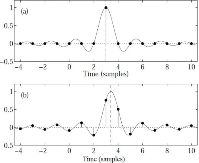
Figure 2.3: Continuous-time (solid line) and sampled (dots) impulse response of the ideal fractional delay filter, when the delay is (a) D= 3.0 samples and (b) D= 3.4 samples. The vertical dashed lines indicate the middle of the continuous-time impulse response in each case……….18

Figure 2.4: The arrangement of a K-channel filter bank with a decimation factor N………21

Figure 3.1: A general Sub-band Adaptive Beam forming (SAB) structure with a Generalized Side lobe Canceller (GSC) at each set of the sub-bands………22

Figure 3.1.1: Signal, noise and microphones position………..23

Figure 3.2.1: LMS adaptive beam forming network………25

Figure 4.1.1: Structure of Generalized Side lobe Canceller………..30

Figure 4.2.2: The blocking matrix obtained by S cascaded columns of differencing………33

Figure 4.3: General SAF structure, where sub-band splitting and full-band error reconstruction is performed by the filter banks……….35

Figure 4.4: A general sub-band adaptive beam forming structure………36

Figure 4.5: A general SAB structure with a GSC in every sub-band………37

Figure 5.2: SNR measurement scenario……….39

Figure 5.3.2.2: Original signal, signal with noise in microphone-1………..41 Figure 5.4: Original signal, Mic1 signal with noise, output signal at GSC………45 Figure 5.5.3: Noise reduction rate after using LMS and NLMS algorithm………47 Figure 5.5.4: Noise reduction rate after using LMS and NLMS algorithm with DFT matrix...48 Figure 5.5.5: Noise reduction rate after using LMS and NLMS algorithm with Hadamard matrix………..48

Chapter 1

Introduction

Some challenging speech applications, such as videoconferences and smart-rooms, might use microphones that can be several meters away from speakers. In these conditions recorded signals are severely degraded by noise and reverberation, and usually some kind of processing is necessary to enhance the speech signal [1].

Adaptive beam forming is becoming increasingly important in acoustical applications. Beam forming can be applied to multiple sound sources, which can be divided into two groups: main signal and noise signals. The purpose of beam forming is to enhance a target signal while suppress the noise signals. One of the good acoustical applications in video conferencing, where a speaker is the main signal and the noise sources that are in the same room seen as jammers [2]. Adaptive beam forming based on a GSC has been widely considered because of its effectiveness and simplicity for achieving multiple linearly constrained beam forming and partially adaptive beam forming. However, many reports show that the GSC-based adaptive beam formers are usually very sensitive to the mismatches in steering angle and weight vectors [3].

1.1 Problem Statement

In this project, my aim is to analyze, design and implement a 4-channel microphone array that is an adaptive sub-band GSC beam former in a noisy environment for speech enhancement as well as SNR improvement using LMS and Normalized LMS algorithm.

1.2 Aim of the Thesis work

The first aim of this thesis is to understand speech enhancement in a noisy environment approaches, most importantly have a thorough understanding of a fully adaptive sub-band GSC beam forming based on LMS and Normalized LMS algorithm. The focus of this thesis will be an investigation of adaptive algorithms. The investigation includes a study of fractional time delay filtering, sub-bands, GSC, different blocking matrixes etc.

The main contributions of this thesis are:

 Modeling an adaptive sub-band GSC beam forming for noise reduction as well as speech enhancement with the help of LMS and Normalized LMS algorithm in adaptive section.

 Noise suppression using different blocking matrixes, variable step sizes, different noise locations with variable SNR in noise.

 Implementation on MATLAB.

 Method validation by the simulation.

1.3 Organization of Thesis

The first chapter has already provided an introduction, aim of the thesis work and main contributions. Chapter two will provide a discussion on literature review where mainly focus on basics of beam forming, fractional time delay filtering and fundamentals of sub-band approaches. Chapter three describes about problem formulation, description of LMS algorithm and Normalized LMS algorithm. Chapter four briefly discusses about GSC, target signal, noise and microphone‟s position, blocking matrix design and generalized sub-band adaptive beam forming. Chapter five provides a detailed understanding of the system block diagram, SNR measurement scenario, simulations, extracted data from the simulation and their analysis. Chapter six concludes the thesis with a summary and scope for future research in the area of adaptive sub-band GSC beam forming for noise suppression in an acoustic environment.

Chapter 2

Literature Review

2.1 The Basics of Beam forming

Beam forming is one of the good methods to combined sound or electromagnetic signals in the process, from only a specific direction and contact of different sensors at the receiver. Since the phase coherence with appropriate compensation, the signals generated at each sensor to provide a higher intensity in the resultant signal. Therefore, the sensor's final gain signal looks like a big dumbbell-shaped lobe to the way of interest. This significant idea is used in different communication, sonar and audio /video voice applications. Normally, beam former is essentially a directivity measure. Beam forming is the process of trying to focus on a particular direction where signal is coming from that direction. It looks like a large dumbbell-shaped expected in the direction of importance which shown as Figure in 2.1[9].

Figure 2.1: Visualization of a realistic beam former.

Beam former includes the sensor array in a specific configuration. The outputs of each sensor are the correctly filtered and after that outputs (filtered) of all the sensors are added together. The second very important advantage of using a sensor array of spatial filtering flexibility provided

by the discrete sampling. The typical beam forming used to form in sonar, radar, communications, imaging, geophysical investigation, biomedical, source localization etc [4].

2.1.1 Delay and Sum Beam forming

Simple delay and sum beam former is a model of data-independent beam forming. Delays and sum beam forming, the delay are inserted after each microphone to make up for the arrival time difference of the speech signal of each microphone (Figure 2.2.1). Time alignment delays of the output signal are then summed. This is to enhance the desired speech signal at the same time as the unnecessary off-axis noise signal is more unpredictable combination of effects. The SNR of the total signal is superior than (or in the worst case, equal), any individual microphone signals. The system makes a more sensitive to the source of the desired array pattern from a particular direction.

The main drawback of the delay and beam forming systems is a lot of sensors needed to improve the SNR. The increase in the number of sensors will provide an additional 3 dB increase in SNR, and this will happen when the incoming interference signals are totally uncorrelated between the sensors and with the desired signal. Another drawback is that no nulls are located directly placed in the position of the interference signal. The purpose of delay and sum beam forming, in order to improve the signal in the direction where the array is currently steered[4].

Figure 2.1.1: Delay and Sum beam former with J sensors.

)

(k

Y

)

(

k

X

2.1.2 Filter-Sum Beam forming

The delay and sum beam former fit in to a more common class which is called the filter sum beam formers, where amplitude and phase weights both are frequency dependent. In practice, most of the beam formers are a kind of filter and sum beam former. Its output is like as below [5].

The structure of a general filter-sum beam former‟s block diagram is given in Figure 2.1.2 [5]

2.2 Adaptive Beam forming problem setup

Figure 2.2: Top view of a smart microphone system utilizing a uniform linear array of 4 microphones.

An adaptive beam former, shown in Figure 2.2, consists of multiple microphones such as 4 microphone; complex weights, the function of which is to amplify (or attenuate) and delay the signals from each microphone element; and a adder to add all of the processed signals, in order to tune out signals not of interest, while enhancing signals of interest.

2.3 Fractional Time Delay Filtering

In classic applications of fractional delay (FD) filters, interpolation between samples is required and uniform sampling is used. Fractional delay, which is a non-integer multiple of sampling interval delay. Employ FD filters to facilitate the use of traditional well-known uniform sampling of signal and signal values at random locations between the samples [6].

A digital edition of a continuous-time delay line is a perfect fractional delay element. The delay system must provide band limited using an ideal low-pass filter at the same time as the delay is only transferred in the time domain impulse response. Therefore, an ideal fractional delay filter‟s impulse response is the transferred and sampled of the sinc function, that is h (n) =sinc (n-D), where

Figure 2.3: Continuous-time (solid line) and sampled (dots) impulse response of the ideal fractional delay filter, when the delay is (a) D= 3.0 samples and (b) D= 3.4 samples. The vertical

n is the (integer) sample index and D is the delay with an integer part floor (D) and a fractional part d=D-floor(D). The floor function returns the greatest integer less than or equal to D. Figure 2.3 shows the ideal impulse response, d = 0.0, d = 0.4 sample. In the latter case, the impulse response length is unlimited. For this reason, the impulse response corresponding to a non-causal filter cannot be ready causal for a finite shift in time. The filter is not absolutely stable. A number of finite-length, causal approximation for the sinc function has to be used for produce a realizable fractional delay filter[6].

One of the finest solutions for the target is a FD all-pass filter. The filter can be applied group delays in samples in the entire audio spectrum. In different types of FD filters, one could satisfy the requirements in the maximally flat. A discrete-time all-pass filter‟s transfers function as follows:

=

(2)

Where N is the filter order and the coefficients of filters,

a

coefficients

a

(3) Where

Specify the K th binomial coefficient. The coefficient a0 is all the time 1, there is no need to

normalize the coefficient vector [7].

Thiran (1971) showed that if D>N; the roots of the denominator (poles) are within in the complex plane unit circle. This means that the filter is stable. The filter is also stable when N-1<D<N. The nominator is a mirrored version of the denominator and the poles are inside the unit circles as well as the zeroes are outside the unit circle. Zeroes and pole‟s angles are the same, but the radius is inverse of each other. For this reason, the filter amplitude response is flat. It is likely to say [8]:

2.3.1 The Order of the Filter

The order of the filter depends on the required time delay and sampling rate, the sample was taken from the group delays. The order of the filter can be calculated as follows:

N = Time delay * sample rate (5)

N has been rounded to the nearest integer number. Such as the concern to create a time delay of 2.5095 ms at the sampling rate 16KHz, the filter order is N=40. With this filter order we can make a delay over an audio signal which has been sampled at 16KHz, between 39.5 and 40.5 samples. The correctness of delay depends on the numbers of the separated steps in this field[8].

2.4 Fundamentals of Sub-band:

When the full band signal is dividing into sub-bands, sample it at a lower rate due to the reduced bandwidth. The resultant individual sub-bands can be dealt with independently in further processing, such as audio coding. These sub-band signal processing can be reconstructed using the synthesis filter bank to acquire a full band system output at the basis sampling rate. Usually different sampling rates are employed in different parts of the system; they are also known as multi-rate filter bank.

There are two major merits for using sub-band adaptive beam forming. First one is for reduced computational complexity due to a lower sampling rate at the decimated sub-bands and other is the convergence speed which was happened due to the pre whitening result of the sub-band decomposition [10].

Figure 2.4 shows the arrangement of a K-channel filter bank with a decimation factor of N, where the inputs signal x[n] is decomposed into K sub-bands by an analysis filter bank H0 (z)…

Figure 2.4: The arrangement of a K-channel filter bank with a decimation factor N.

Chapter 3

Problem Formulation and Algorithm

3.1. Overall System

An overview of the whole system will be presented. After that a detailed explanation of every step will be given in order to better understand. Figure 3.1 summarizes the process.

Figure 3.1: A general Sub-band Adaptive Beam forming (SAB) structure with a Generalized Side lobe Canceller (GSC) at each set of the sub-bands.

Figure 3.1 shows a general SAB structure, where each of the M received array signals xm[n], m =

0, 1,...,M −1 is decomposed into K sub-bands by a K-channel analysis filter bank and a GSC beam former is then set up at each set of the M corresponding decimated sub-band signals. The output yk [n], k = 0, 1... K −1, of these K sub-band beam formers are then combined by a

synthesis filter bank to form the full band output y[n].

In Figure 3.1, the blocks labeled „A‟ are the analysis filter banks (including the down-sampling) and the block labeled „S‟ is the synthesis filter bank (with up-sampling). In total there are M analysis filter banks and one synthesis filter bank.

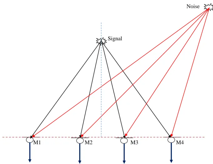
As mentioned in the earlier sections, the main target is to obtain the better SNR as well as speech enhancement in a noisy environment where from a signal source is emitting a voice signal which was situated at in front and middle of microphones and noise was taken from right or left of main signal source. SNR improvement has been verified to putting voice signal and noise source in different location and one of its sample figures is shown in below.

Y noise (3, 2) Noise (-3, 1.5) Signal (0, 1) -X M1 (-0.075, 0) M2 (-0.025, 0) M3 (0.025, 0) M4 (0.075, 0) X d= 0.05m

Figure 3.1.1: Target signal, noise and microphones position.

To achieve that, the system shown in Figure 3.1.1 was designed in Mat Lab code. After used the fractional time delay filter in both voice signal and noise were captured by the microphones then split each of the microphones signals into sub-bands and applied GSC to each of the corresponding sub-bands and take the overall SNR improvement with verified by the different scenarios.

This chapter provides a detailed understanding of the working of the Least Mean Square algorithm (LMS) and Normalized LMS algorithm in section 3.2 and then in section 3.3 the next steps leading to obtain the direction.

3.2. General approach

The LMS algorithm was invented by Bernard Widrow and Ted Hoff in 1959[12]. The LMS is algorithms are a class of adaptive filter used to mimic a desired filter in which a simplification of the gradient vector computation. This algorithm is widely used in various applications of adaptive filtering due to its simplicity in computational complexity. Compared with others LMS algorithm is relatively simple, it requires no correlation function calculation and not require matrix inversions.

The LMS algorithm is by far the most widely used algorithm in adaptive filtering for several reasons. The best features that attracted the use of the LMS algorithm is the low computational complexity, evidence of convergence in the stationary environment, unbiased convergence in the mean to the Wiener solution and stable behavior when implemented with finite precision arithmetic[13].

3.2.1. The LMS algorithms and adaptive arrays

Consider a Uniform Linear Array with M microphone elements, which forms the integral part of the adaptive beam forming system as shown in the figure below [14].

The output of the microphone array X (n) is given by,

Figure 3.2.1: LMS adaptive beam forming network.

S(n) denotes the desired signal arriving at in front and middle of microphones and N(n) denotes interfering signals arriving at either left or right of microphones. Therefore it is required to construct the desired signal from the received signal and the interfering signal N (n).

As stated above, the outputs of the individual microphones are linearly combined after being scaled by the corresponding weights so that the microphone pattern is optimized to have maximum gain in the direction of the desired signal and null in the direction of the noise signal. The weights here will be calculated using the LMS algorithm based on Minimum Squared Error (MSE) criterion [14].

Therefore, spatial filtering problem involves the estimation of the signal s(n) from the received signal x(n) (i.e. the array output) by minimizing the error between the reference signal d(n), which is nearly matches or have some correlation with the desired signal estimation and beam former output y(n). This is a classic Weiner filtering problems where the solution can be iteratively found using the LMS algorithm.

3.2.2. Formulation of the LMS algorithm

According to steepest descent, the weight vector equation is given by [15],

w (n+1) = w (n) -

μ

Where μ is the step size parameter and controls the convergence properties of LMS algorithm; e2(n) is the mean square error between the beam former output y(n) and the reference signal which is given by,

e2 (n) = [d*(n)-wH x (n)] 2 (8)

The gradient vector in the above equation can be computed as

(n)}) = -2r+2 Rw(n) (9)

In the method of steepest descent the main problem is the calculation to find the values of r and R matrices in real time. LMS algorithm, on the other hand, simplifies this by using the instantaneous values of the covariance matrices r and R instead of their native values i.e.

R (n) = x(n) xH (n) (10)

r (n) =d*(n) x(n) (11)

Therefore the weight update equation can be given by the following way,

w (n+1) = w(n)+μx(n)[

w(n)+μx(n)

The LMS algorithm initiated with an arbitrary value w(0) for the weight vector at n=0.The gradual correction of the weight vector leads eventually to the lowest value of the mean squared error.

Therefore the LMS algorithm‟s equations can be summarized in following way;

Output, y (n) = wH x(n) (13)

Weight update equation,

w(n+1)

w(n)+μx(n)

3.2.3 Convergence and Stability of the LMS algorithm

Optimum value for the step size would be [16]:

μ

=

and

The convergence of the algorithm is inversely proportional to the Eigen value spread of the correlation matrix R(n).When the Eigen values of R(n) is large, convergence can be slow. The Eigen value spread of the correlation matrix is estimated by calculating the ratio of the largest Eigen value to the smallest Eigen value of the matrix. If μ is chosen to be very small then the algorithm converges very slowly. A large value of μ can lead to a faster convergence, but may be less stable around the minimum value [14].

3.3 Normalized LMS (NLMS) algorithm

The Normalized LMS (NLMS) introduces a variable adaptation rate which improves the

convergence speed in a non-static environment [14].

In the design and implementation of the LMS adaptive filter one is problem is the choice of the step size μ. For the stationary process, the LMS algorithm convergence in the mean if 0< < 2/ , and convergence in the mean –square if 0< < 2/tr (Rx) .Since Rx is generally unknown,

then either or Rx must be estimated in order to use these bounds. One way about this

difficulty is to use the fact that, for stationary processes tr (Rx) = ( +1) E , p is the filter

order. Therefore, the condition for mean-square convergence is replaced by [23] 0<μ<

Where E is the power in the procedure x (n). This power may be anticipated using a time average such as

{ } = (16) This leads to the subsequent bound on the step size for mean-square convergence:

0<μ<

A suitable way to integrate this bound into the LMS adaptive filter is to use a (time changeable) step size of the form

μ (n)= =

(17)

Where is the normalized step size with .Replacing μ in the LMS weight vector updated equation with μ(n) lead to the NLMS algorithm, which is specified by:

Wk (n+1) = Wk (n) +

(18)

(Where “*” represents the conjugate value and “ ” is the normalized step size)

The effect of the normalization by is to alter the magnitude but not the direction of the estimated gradient vector. The appropriate set of statistical assumption it may be exposed that the NLMS algorithm converges in the mean square if .With the normalization of the LMS step size by in the NLMS algorithm, on the other hand, this noise amplification difficulty is diminished and it bypasses this problem [23].

Chapter 4

Generalized Side lobe Canceller and Full System Overview

4.1 Generalized Side lobe Canceller (GSC)

Data dependent beam forming techniques try to adaptively filter incoming signals to pass the signal from the desired direction while rejecting noises from other directions. For their minimization criterion, most adaptive techniques rely on the optimization of mean-square error between a reference signal that is highly correlated to the desired signal and the output signal [5]. The GSC is a simplification form of the Frost algorithm which was presented by Griffiths and Jim about ten years after Frost's original paper was published [18].They proposed an alternative, but effective implementation of the LCMV beam former, which is called the GSC. It can be considered as a system for transforming the constrained minimization problem into an unconstrained one [10].

4.1.1 Structure of GSC

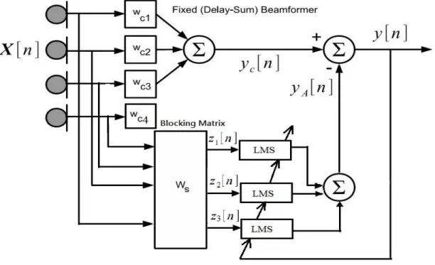
Displayed in figure 4.1.1[19], the structure consists of two parts which is called upper part and lower part. In the upper part often called the fixed beam former and the lower part consisting of adaptive section along with blocking matrix.

Figure 4.1.1: Structure of Generalized Side lobe Canceller.

In the adaptive section, this is a combination of a set of filters that adaptively minimize the power of the output. The desired signal is eliminated from the second path by a Blocking Matrix (BM), ensuring that it is the noise power that needs to minimize.

The upper portion is called a fixed beam former because of its behavior which is constant over time. The constant wc may be chosen any non zero values but are almost chosen always as

normally , yielding from delay and sum beam former:

[n] = (19)

(Assume that the microphones have already been target-aligned. In more, now need to adopt the more common practice of referencing the input data and weights value of tap which is not as vectors but as matrices where each column represents to data for an individual sensor and each row correspond the data for all sensors).

The lower path of the structure is the adaptive part. It consists of two major parts. The first of these is the blocking matrix W_s, whose purpose is to remove the desired signal from the lower path. Since the desired signal is common to all the time - in line inputs, block will occur if the rows of the blocking matrix sum to zero and the rows are linearly independent[5].

As a result X[n] can have at most M-1 linearly independent components such as microphones or sensors. Equivalently, the row dimension of Ws must be M - 1 or less. The standard Griffiths-Jim

BM is [18]

Ws =

For these Ws, the BM outputs are computed as the matrix product of the BM and matrix of current input data.

Z[n] = X[n] (20)

The overall beam former output, y[n], is computed as the fixed beam former signal minus the lower branch data which is came from the blocking matrix output and adaptive section

y[n] = [n] - (21)

Where Wk[n] is the kth column of the tap weight matrix W and

z

output and these two matrixes has same length. In the adaptive filters weight updated using the LMS algorithm with reference signal as y[n]

Wk [n+1] = Wk[n] +

μ

(Where “*” represents the conjugate value and “

μ” is the step size

When concern about NLMS algorithm in the GSC, weight update equation is like as below:

Wk [n+1] = Wk[n] +

(23)

(Where “*” represents the conjugate value and “ ” is the normalized step size which value is between )

The GSC is a flexible structure due to the separation of the directional microphone in a fixed and adaptive part, and it is the most widely used adaptive beam former. In experiment, GSC causes some distortion of the desired signal, due to a phenomenon called signal leakage. Signal leakage occurs when the BM does not remove entire desired signal from the lower path. This can be

especially problematic for broadband signals, as it is difficult to ensure perfect signal cancellation over a wide frequency range [5].

4.2 Blocking Matrix Design

The structure of the BM, Ws plays an important role in the GSC structure, its choice

determines the computational complexity and in many cases, strengths against numerical instabilities of the overall system [20]. The GSC structure requires finding the proper quiescent vector Wc and a blocking matrix Ws that meets the constraints. The design of a proper BM can

be obtained by invoking the cascaded columns of differencing (CCD) or singular value decomposition (SVD) [21].

4.2.1 Singular Value Decomposition (SVD)

Singular value decomposition (SVD) is a very good tool in linear algebra. Application of SVD in the GSC beam former is to formulate the BM and the pseudo inverse for the quiescent vector [21].

The SVD theorem says that given a matrix A, there are two uniform matrices U and V, so we have:

A=U VH (24) Where is an r x r diagonal matrix, contains the ordered singular values which are positive definite of A. The variable r is the rank of A and represents the number of linearly independent columns in this matrix.

Let us make separate matrix U into two parts like as below:

U= (25)

Where Ur is the first r columns of the matrix U, while holds the remaining columns of U, and

then it is easy to see that:

= 0 (26)

The SVD approach is not limited to broadside limitations case and can applied to any constraint matrix C. Therefore, it is a general strategy for obtaining BM [10].

4.2.2 Cascaded Columns of Differencing (CCD)

The CCD method has been proposed to obtain BM for derivative constraints. Derivative constraints for increased durability against look-direction errors by increasing the angular range of targeted constraints. The higher the order of the derivative constraints, the wider the beam pointing in the desired direction [21].

In the CCD method, the BM is formed by S cascaded columns of differencing operations as shown in Figure 4.2.2 [10].

In matrix form, the BM formulated as below: = BM . BM-1 … BM-S+1 (27) Where we have Bi=

With i = M, M-1. . . M-S-1. Clearly, if the signal of interest comes from the wide side, it will not be possible to pass through such an above BM. The Zero response formed by the BM in broadside will have a wider lobe width with increasing S [10].

4.3 Sub-band Adaptive Beam forming

In microphone array, if we received the wide bandwidth signal, different sub-band decomposition techniques can be used in the beam forming process for better performance. The two advantages of sub-band adaptive beam forming are a reduced computational complexity, due to the lower sampling rate in the decimated sub-bands and the convergence rate increases, due to the effect of sub-band decomposition of pre-whitening [10].

Sub-band technique usually involves two sets of filters used. The first group is the sub-band decomposition, so that the necessary processing such as beam forming, can be performed at resultant sub-bands and for the second group is the reconstruction of the whole band, where all the sub-band signal together to form the original full-band . When the full-band signal is split into sub-bands, then we can sample it at a lower rate, due to reduced bandwidth of the sample. The resulting individual sub-band can be regarded separately during further processing such as audio coding [10].

The general sub-band adaptive filter (SAF) system as shown in Figure 4.3, where input signal and the desired signal both are split into decimated sub-bands by analysis filter banks and then with the sub-band adaptive filters like as Windowed Discrete Fourier Transform (WDFT), running on a lower rate compared to the original full-band system is used to estimate the sub-band desired signals using the sub-sub-band input signals. The resulting sub-sub-band error signals are then reconstructed into a full-band error signal by a synthesis filter bank [10].

Figure 4.3: General SAF structure, where sub-band splitting and full-band error reconstruction is performed by the filter banks.

The Windowed Discrete Fourier Transform (WDFT) of x[n] can be obtained as [22]

X [m, wi] =

(28)

Where, wi=

, i=0…N-1, and S[n] is a window function. In the framework of filter banks, X [m,wi] can be regarded as the i:th sub band signal (often denoted Xi[m]).

The inverse WDFT is usually given as

[Mm+n]=

(29)

Where, K= overlapping ratio (N/M). When K=2 then there is 50% overlap. N= no. of samples in each block.

M= no. of sub-bands.

4.4 General Sub-band Adaptive Beam forming

In the Sub-band adaptive beam forming (SAB), the basic idea is to first receive the sensor signal then split the signals into different sub-bands, and then implement an independent beam former in each separate of them, with the sub-band beam former selected according to the specific applications [10].

Figure 4.4: A general SAB structure [10].

Figure 4.4 shows a general structure of the SAB, where each row of M received signals xm [n], m

= 0, 1,..., M - 1 is broken down into K sub-bands with a K-channel analysis filter bank and after that in each sub-band an individual beam former is setup. The output yk [n], k = 0, 1... K - 1,

these K sub-band beam formers are then combined by a synthesis filter bank to form a full band output signal y [n].

Depending on specific applications, we can choose a GSC, or a reference signal based beam former, or any other suitable ones [10].

4.5 Sub-band Adaptive Generalized Side lobe Canceller (GSC)

When we have idea about the direction of arrival of the signal of interest, we can employ a GSC at every set of sub-bands for beam forming and the structure is shown in below figure 4.5 [10].

Figure 4.5: A general SAB structure with a GSC in every sub-band.

In sub-band adaptive beam forming which is based on a GSC, it was limited to using the same number of analysis filter banks as the same microphone number M, and also the same number of GSC‟s as sub-band number K, as we have to divide each microphone signals into sub-bands and apply a GSC to each of the correspondent sub-bands. When the number of microphone arrays and sub-bands are high, these operations represent a high computational load on the system. Furthermore, in this method, full-band limitations of the beam former must be split into sub-band based constraints to build a GSC for each sub-band. This forecast may lead to inaccuracies due to the non-perfect reconstruction property of the filter banks and the limited number of weights to represent the constraints in each sub-band [10].

For the computational complexity of the sub-band beam former, it can also be divided into two parts, first one is the filter banks part and second one is the sub-band GSC. If there is M analysis filter banks and one synthesis filter bank. Then the total number of real multiplications for the filter banks is (M + 1) / N (lp + 4K log2 K + 4K) or (M + 1) / N (2lp + 4K log2 K +8K) for real and

Chapter 5

System Design and Simulation

5.1 System Block Diagram

noise noise signal

M1 M2 M3 M4

Main signal and noise was taken in every sensor‟s by fractional time delay filter. In microphones over all signal, implemented the Sub-band technique.

Implement GSC (Generalized Side lobe Canceller) in each sub-band.

In GSC‟s adaptive section:

implemented LMS algorithm. In GSC‟s adaptive section: _{implemented Normalized}

LMS algorithm. Taken the overall SNR improvement Taken the overall SNR improvement Used different types of

BM for suppression the desired signal in the lower part of GSC.

5.2 SNR Measurement Scenario

SNR measurement has been taken in the following ways: Signal power_d(n)

Signal power out_e (n)

Copied copied Signal Copied d (n) + e(n) y (n)- Copied Copied

Noise Noise power_d (n) Noise power out_e (n)

Figure 5.2: SNR measurement scenario. WC Blocking Matrix (B) Wa Wa Wa Signal & Noise WC Blocking Matrix (B) Wa Blocking Matrix (B) Wa WC

Based on the above figure, SNR calculations like as following ways:

SNR1=

SNR2=

5.3 Simulations & Result Analysis

After designed the above SNR measurement scenario for noise cancellation as well as SNR improvement, the following simulation were carried out for test the system. Each group of tests were done to verify that a particular part of the program or worked throughout the program properly. The results are exposed and explained in the order they were accomplished.

5.3.1 Original signal

The system was built in two stages methods. Two groups of signals were experienced: speech signal and sinusoidal complex signal. Voice signal such as .wav signal is used with 8 kHz sampling rate. In the system, used by 4 microphones with linear array and signal was came from the middle and in front of microphones with co-ordinate is (0, 1) in the Y-axis. Inter space distance between microphone was 0.05m and 4 microphones co-ordinate was M1 (-0.075, 0), M2 (-0.025, 0), M3 (0.025, 0) and M4 (0.075, 0).

5.3.2 Random noise

In simulations, used the additive white Gaussian noise like as random having mixing with a different SNR (3dB, 5 dB, 10dB, 15dB) i. e, this SNR is mixing with noise with different times for measuring the overall SNR improvement. Noise has been taken approximately 450/1200 degree angles like as co-ordinates was (3, 2), (3, -2), (2.5, -1.5), also in different directions and locations.

Figure 5.3.2.1: Position of Microphone arrays, source signal and noise.

In each of the microphone, source signal and noise was captured after implemented by fractional time delay filtering like as thiran approximation. Every microphone‟s captured target signal and noise both. Below figure 5.3.2.2 is showing the target signal and signal with noise in microphone 1.

After received every microphone‟s signal additive with white noise then divide each of the sensor signal into sub-bands and apply a GSC to each of the corresponding sub-bands for measurement the SNR improvement. In the GSC‟s adaptive section, implemented LMS and NLMS algorithm for noise reduction.

5.3.3 Selection of Conventional Beam former and Different Blocking Matrix

According to the figure 4.1.2, In the GSC, there are two different substructures which are the upper and lower processing paths. The upper or conventional beam former path consists of a set of fixed amplitude weights wC1, wC2, wC3, wC4, which produce non- adaptive beam formed

signal yc[n][18].

One widely method uses Chebyshev polynomials to find Wc. Any method can be used to select

the weights as the performance of on the whole beam former will be characterized in terms of the chosen specific values. To simplify notation, the coefficients in Wc, is normalized to have a sum

of unity [18] i.e, [wC1, wC2, wC3, wC4] = [1, 1, 1, 1] and it is doing as averaging.

In the lower branch there is also two section, one is BM and another is working like as Adaptive Noise Canceller (ANC), which is a well known speech enhancement technique. For the lower branch, while the desired signals are blocked due to passed through the BM section, only interfering signals and noise be able to pass. When adapting wa to reduce the variance or power

of the output signal y[n], the system will be likely to cancel the interference and noise component in the upper section only [10].

Different BM has been taken and implements this in my system and measure the SNR improvement. Due to this course, here we are mentioning some examples of this.

BM is required to have M-1 linearly independent rows that‟s sum up to zero, where M is the no of sensors. Many matrices can be generated using this characteristic, there are two possibilities, concerning only addition operations are shown below for the case M = 4 [18]:

(1) = (30) (2) = (31)

In the first matrix the rows are mutually orthogonal and Walsh function of the binary valued of the element, the second matrix involves less operation and includes the difference between adjacent microphone outputs [18].

Concerning about spatial null in the desired direction and a zero derivative in that path. Below matrix (3) will fulfill the result for M = 4.

(3) = (32)

Above matrix‟s row dimension is M-2, due to the additional spatial restriction. The system sensitivity to time-delay steering errors, but it is markedly reduced [18].

Hadamard functions are rectangular or square wave forms with values of -1 or +1. An important feature of these functions is sequence which is determined from the number of zero crossings per unit time interval. It has a unique sequence value [24].Below matrix (except the first row) (4) from the Walsh transform for M = 4 [25].

(4) = (33)

Another one taken from the Discrete Fourier Transform matrix (except the first row) [26].

(5) = (34)

Here giving the SNR improvement as well as noise suppression. This result collected by implemented different BM and in the GSC‟s adaptive section using with LMS algorithm. Sampling frequency was 8 KHz and microphone‟s inter distance was .05m. Simulated several times and take the SNR improvement.

5.4 SNR Measurement by LMS Algorithm

Given Conditions Trial 1 Trial 2

Blocking matrix Input SNR

Filter Order

Position of

Noise signal Step size d_n (dB) GSCout (dB) d_n(dB) GSCout (dB)

[1 -2 1 0;0 1 -2 1;1 0 1 -2] 3 1 (X,Y)= (3,2) _5.00E-02 9.0522 11.8996 9.0833 11.8042 5 1 (X,Y)= (3,2) 5.00E-02 11.0246 13.3187 10.9617 13.0004 3 4 _{(X,Y)= (3,-2) 5.00E-03} 8.9208 11.6741 8.9292 11.6123 3 8 _{(X,Y)= (3,-2) 5.00E-03} 8.9567 11.4515 8.9455 11.4683 5 16 _{(X,Y)= (3,2) 5.00E-04} 10.933 13.2783 11.0495 13.1933 5 32 _{(X,Y)= (3,2) 5.00E-04} 10.9264 12.9985 10.9596 13.2104 10 1 (X,Y)= (3,2) 5.00E-02 15.9764 16.1743 16.0285 16.582 10 32 _{(X,Y)= (3,2) 5.00E-04} 15.9492 16.0066 16.0116 16.6763 [1 -2 1 0;0 1 -2 1;1 1 -1 -1] 3 1 _{(X,Y)= (3,1.5) 5.00E-02} 9.1553 12.1665 9.1235 12.0619 3 16 (X,Y)= (3,1.5) 5.00E-03 9.1619 12.2027 9.1206 12.0324 5 4 (X,Y)= (3,2) 5.00E-02 10.9438 13.9073 10.9728 13.7708 5 16 (X,Y)= (3,2) 5.00E-03 10.9743 13.7609 11.021 13.674 5 32 (X,Y)= (3,-2) 5.00E-04 10.9976 13.8223 10.9122 13.425 10 16 (X,Y)= (3,1.5) 5.00E-02 16.1053 17.5524 16.1351 17.6948 [1 -1 -1 1;1 -1 1 -1;1 1 -1 -1] 3 1 _{(X,Y)= (3,2) 5.00E-02} 8.9821 11.7535 8.9752 11.7845 3 16 _{(X,Y)= (3,2) 5.00E-03} 9.0321 11.6939 8.9016 11.6499 5 4 (X,Y)= (3,2.5) 5.00E-03 10.7724 13.0807 10.7231 13.4655 5 16 (X,Y)= (3,-2) 5.00E-04 10.9471 13.4345 10.9357 13.3331 5 32 (X,Y)= (3,-2) 5.00E-02 10.9641 13.4244 10.8947 13.3386 5 64 (X,Y)= (3,-2) 5.00E-03 11.0411 13.2272 10.9552 13.4603 10 4 (X,Y)= (3,1.5) 5.00E-03 16.1316 16.5705 16.1671 16.6773 [1 -1 1 -1;1 1 -1 -1;1 -1 -1 1] 3 1 _{(X,Y)= (3,2) 5.00E-02} 8.9321 11.706 8.9449 11.5357 3 16 (X,Y)= (3,-2) 5.00E-03 9.0069 11.7467 8.9527 11.3963 5 4 _{(X,Y)= (3,1.5) 5.00E-04} 11.0495 13.3301 11.0763 13.3791 5 16 (X,Y)= (3,2) 5.00E-03 10.9172 13.3917 10.9869 13.3036 5 32 _{(X,Y)= (3,2.5) 5.00E-02} 10.7502 13.222 10.7036 13.1297 5 64 (X,Y)= (3,1.5) 5.00E-03 11.0654 13.424 11.0777 13.2858 10 4 (X,Y)= (3,2) 5.00E-02 15.9717 16.0368 16.0368 16.3429 [1 1 -1 -1;1 -1 -1 1;-1 -1 1 1] 3 4 _{(X,Y)= (3,2) 5.00E-03} 8.8785 11.4175 8.9251 11.2543 3 16 _{(X,Y)= (3,-2) 5.00E-02} 8.8885 11.3021 9.0178 11.4096 3 32 (X,Y)= (3,2.5) 5.00E-02 9.1464 11.6137 9.1269 11.5703 5 1 _{(X,Y)= (3,2) 5.00E-04} 10.9949 13.266 11.0209 13.2682 5 4 (X,Y)= (3,-2) 5.00E-02 10.9255 12.7532 10.9812 12.9287 8 16 (X,Y)= (3,2) 5.00E-02 13.7608 14.746 13.8423 14.7031 10 4 (X,Y)= (3,1.5) 5.00E-03 16.0954 16.1132 16.062 15.9503

Based on the above table 5.4.1, after implemented by LMS algorithm in the GSC‟s, overall SNR improvement about 9 or 10 dB.

After implemented LMS algorithm, then implemented the NLMS algorithm and take the SNR improvement. Below figure 5.4 is showing the output signal at GSC. In Mic1, mixed up with main signal and noise both.

5.5 SNR Measurement by NLMS Algorithm

Blocking matrix Input SNR Filter Order Position of Noise signal Step size d_n(dB) GSCout(dB) d_n(dB) GSCout(dB)

[0 1 -2 1; 1 -2 1 0; 1 1 -1 -1] 3 4 (X,Y)= (3,-2) 5.00E-04 10.5338 13.8077 10.5415 13.9558 3 8 _{(X,Y)= (3,2) 5.00E-04} 10.6211 13.1682 10.4559 13.0848 3 16 _{(X,Y)= (3,2)} 5.00E-03 10.5052 15.3183 10.4928 14.7226 3 32 _{(X,Y)= (3,2) 5.00E-04} 10.4169 13.627 10.3321 13.7984 5 4 _{(X,Y)= (3,-2)} 5.00E-03 12.6135 16.0692 12.5371 15.8578 5 8 _{(X,Y)= (3,2) 5.00E-04} 12.4359 15.7997 12.5162 15.8167 10 4 _{(X,Y)= (3,-2) 5.00E-02} 17.6414 20.4693 17.3914 19.6926 10 16 _{(X,Y)= (3,-2) 5.00E-04} 17.5944 19.0959 17.5551 18.9998 [1 -1 -1 1;1 -1 1 -1;1 1 -1 -1] 3 4 (X,Y)= (3,-2) 5.00E-04 10.4858 13.7659 10.5448 13.8129 3 8 _{(X,Y)= (3,2) 5.00E-03} 10.3222 13.2973 10.5483 13.5892 5 4 _{(X,Y)= (3,-2) 5.00E-04} 12.5681 15.5945 12.5873 15.8477 5 8 _{(X,Y)= (3,2) 5.00E-03} 12.6151 14.9003 12.5217 14.779 10 4 (X,Y)= (3,-2) 5.00E-04 17.4805 18.1652 17.4335 18.0251 [1 -1 1 -1;1 1 -1 -1;1 -1 -1 1] 3 4 (X,Y)= (3,-2) 5.00E-04 10.5356 13.9629 10.5299 13.8756 3 8 _{(X,Y)= (3,2) 5.00E-03} 10.5404 13.6609 10.3669 13.688 3 16 _{(X,Y)= (3,-2) 5.00E-04} 10.3666 12.523 10.6096 12.3544 3 32 _{(X,Y)= (3,-2) 5.00E-04} 10.5322 11.8143 10.4619 11.5675 5 4 _{(X,Y)= (3,-2) 5.00E-04} 12.3168 15.4446 12.4756 15.6521 5 8 _{(X,Y)= (3,2) 5.00E-03} 12.5443 15.1125 12.5366 15.3515 10 4 _{(X,Y)= (3,2) 5.00E-04} 17.5618 18.5022 17.4033 17.9956 [1 1 -1 -1;1 -1 -1 1;-1 -1 1 1] 3 4 (X,Y)= (3,2) 5.00E-04 10.5897 13.8927 10.4309 13.916 3 8 _{(X,Y)= (3,-2) 5.00E-03} 10.3811 13.3546 10.5519 13.8317 5 4 _{(X,Y)= (3,2) 5.00E-04} 12.4825 15.5721 12.5303 15.6007 5 16 (X,Y)= (3,-2) 5.00E-03 12.4573 14.5474 12.5229 14.7004 10 4 _{(X,Y)= (3,-2) 5.00E-04} 17.45 17.504 17.5225 17.6606 [1 -2 1 0; 0 1 -2 1; 1 1 -1 -1] 3 4 (X,Y)= (3,-2) 5.00E-04 10.5401 14.1529 10.6271 13.9523 3 8 (X,Y)= (3,-2) 5.00E-04 10.5013 13.2245 10.4299 13.0179 5 8 _{(X,Y)= (3,2) 5.00E-04} 12.4332 14.6998 12.4306 14.7926 10 4 _{(X,Y)= (3,2) 5.00E-04} 17.2314 19.7821 17.5945 18.9729 10 8 _{(X,Y)= (3,-2) 5.00E-04} 17.3946 19.8053 17.3237 19.5914 [1 -2 1 0; 0 1 -2 1; 1 0 1 -2] 3 4 (X,Y)= (3,-2) 5.00E-04 10.7031 13.2751 10.6037 13.2879 3 8 _{(X,Y)= (3,-2) 5.00E-04} 10.2817 11.7655 10.5407 12.174 5 4 _{(X,Y)= (3,2) 5.00E-04} 12.3721 14.762 12.5248 14.5169 5 8 (X,Y)= (3,-2) 5.00E-04 12.2776 13.7842 12.4102 13.7664 10 4 _{(X,Y)= (3,-2) 5.00E-04} 17.4319 17.5636 17.3819 17.8942

Based on the table 5.5.1, after implemented by NLMS algorithm, overall SNR improvement about 13 dB.

Here providing some snapshot with comparison that, how much SNR has improved using LMS and NLMS algorithm with different blocking matrix.

Figure 5.5.3: Noise reduction rate after using LMS and NLMS algorithm

Chapter 6

Conclusion and Future works

6.1 Concluding Summary

In this thesis work we have presented and worked on noisy target signal with linear microphone arrays for maximum noise suppression as well as speech enhancement. To fulfill this target, main signal and noise has taken from each of the microphone‟s using via with fractional time delay filter and after that split each of the sensor signals into sub-bands and applied GSC to every set of the sub-bands. In the GSC‟s lower part BM section, different matrix used such as Griffiths and Jim‟s matrix, DFT and Hadamard matrix etc. SNR improvement has been taken based on this matrix which was shown in the last chapter. Blocking matrix [0 1 -2 1; 1 -2 1 0; 1 1 -1 -1], shows the better SNR improvement with compared to other matrix. In the adaptive section of GSC‟s, noise reductions were done by using LMS and NLMS algorithm.

Followed by the previous chapter and according to figures, tables and charts showing the result that, the benefit of this approach is that the sub-band GSC adaptive beam forming significantly improves the speech quality while maintaining a good noise suppression levels up to 13 dB using with NLMS algorithm and about 10 dB using with LMS algorithm. The performance analysis of the system has focused on its strengths and weakness i.e., where it gives high SNR improvement while mixed up with low SNR in the input signals.

6.2 Future Works

The current design of the sub-band GSC beam former is based on the linear microphone

arrays, but may be extended to planar, round or arbitrary geometrics array. This could be achieved by applying appropriate changes in the structure of the blocking matrix for the frequency-domain GSC beam former, and then extend it to overlap-save methods. Additional microphones may improve overall performance; especially in the beam former. In this thesis, simulated the system in offline mode and it can be implemented on real-time in the future. The result of the system contains little background noise so it can be implemented on high interference and noise. The performance of the LMS and NLMS algorithm can be compared with other subtractive type algorithms.

REFERENCE:

[1] A. Abad and J. Hernando. “Speech enhancement and recognition by integrating adaptive beamforming and Wiener filtering”. In IEEE Sensor Array and Multichannel Signal Processing Workshop, SAM, Sitges. Citeseer, 2004.

[2] M. Joho and G.S. Moschytz. “On the design of the target-signal filter in adaptive beamforming”. Circuits and Systems II: Analog and Digital Signal Processing, IEEE Transactions on, 46(7):963–966, 1999.

[3] J.H. Lee and C.L. Cho. “GSC-based adaptive beamforming with multiple-beam constraints under random array position errors”. Signal processing, 84(2):341–350, 2004.

[4] V.C. Raykar. “A Study of a various Beamforming Techniques And Implementation of the Constrained Least Mean Squares (LMS) algorithm for Beamforming”. Department of Electrical and Computer Engineering, University of Maryland, College Park, 2001.

[5] I. McCowan. “Microphone arrays: A tutorial”. Queensland University, Australia, pages 1–38, 2001.

[6] V. Valimaki and T.I. Laakso, “Principles of fractional delay filters”. In icassp, pages 3870– 3873. IEEE, 2000.

[7] V. Valimaki, “Simple design of fractional delay allpass filters”. In Proceedings of the 2000 European Signal Processing Conference, pages 1881–1884, 2000.

[8] P. Parhizkari, “Binaural Hearing-Human Ability of Sound Source Localization,” Master‟s thesis, Blekinge Institute of Technology, Blekinge, Sweden, December 2008.

[9] M.S. Amin, M.R. Azim, S.P. Rahman, F. Habib, and A. Hoque. “Estimation of Direction of Arrival (DOA) Using Real-Time Array Signal Processing and Performance Analysis”. IJCSNS, 10(7):43, 2010.

[10] W. Liu and S. Weiss. “Wideband Beamforming: Concepts and Techniques”. Wiley, 2010. [11] http://www.azimadli.com/Vibman/gloss_hammingwindow1.htm

[12] K.K. Shetty. “A novel algorithm for uplink interference suppression using smart antennas in mobile communications”. PhD thesis, 2004.

[13] P.S.R. Diniz. “Adaptive filtering: algorithms and practical implementation”, volume 694. Springer Verlag, 2008.

[14] http://etd.lib.fsu.edu/theses/available/etd-04092004-143712/unrestricted/Ch_6lms.pdf [15] S.S. Haykin. “Introduction to adaptive filters”. Macmillan New York, 1984.

[16] N.M. Kwok, J. Buchholz, G. Fang, and J. Gal. “Sound source localization: microphone array design and evolutionary estimation”. In Industrial Technology, 2005. ICIT 2005. IEEE International Conference on, pages 281–286. Ieee, 2005.

[17] C.F.Scola and M.D.B.Ortega, “Direction of arrival estimation – A two microphones approach ,” Master‟s thesis, Blekinge Institute of Technology, Blekinge, SE, September 2010. [18] L. Griffiths and CW Jim. “An alternative approach to linearly constrained adaptive

beamforming”. Antennas and Propagation, IEEE Transactions on, 30(1):27–34, 1982. [19] P. Townsend, “Enhancements to the Generalized Sidelobe Canceller for Audio Beamforming in an Immersive Environment” Master‟s thesis, University of Kentucky, Kentucky, UK, 2009.

[20] S. Werner. “Reduced complexity adaptive filtering algorithms with applications to communications systems”. Espoo: Helsinki University of Technology Signal Processing Laboratory, 2002.

[21] C.L. Koh. “Broadband adaptive beamforming with low complexity and frequency invariant response”. 2009.

[22] S. Hosseini, “Mapping Based Noise Reduction for Robust Speech Recognition,” Master‟s thesis, Blekinge Institute of Technology, Blekinge, SE, July 2010.

[23] M.H. Hayes. “Schaum’s outline of theory and problems of digital signal processing”. McGraw-Hill, 1999.

[24]http://www.mathworks.se/products/signal/demos.html?file=/products/demos/shipping/signal/ walshhadamarddemo.html#4

[25] http://en.wikipedia.org/wiki/Hadamard_transform