Metamodelling of a Finite Element Analysis of a Drilling Process with Replaceable Inserts

(1)

METAMODELLING

OF

A

FINITE

ELEMENT ANALYSIS OF A DRILLING

PROCESS

WITH

REPLACEABLE

INSERTS

Master Degree Project in Industrial Systems Engineering One year Level 22.5 ECTS

Spring term 2019

Samy Akrouh Ettaghadouini Supervisor: Tobias Andersson

(2)

Abstract

The aim of this project is to create a metamodel from a drilling tool with replaceable inserts from FEA of the machining process using MATLAB and ABAQUS. This report contains research in drilling and in metamodeling using neural networks and the work from the design of the CAD, through FEA and simulations, to the metamodeling, excluding the optimization.

The work has resulted in a framework where a base FE model of the drill with two inserts that works, but due to time issues and given high cutting speed and feed the results of the FEA and the metamodeling are not very accurate. Therefore, the optimization analysis could not be done. However, it has been shown that feed has a major influence on the inserts temperature than the cutting speed, despite the higher range of this last one.

(3)

ii

Acknowledgements

I would first like to thank my thesis supervisor Tobias Andersson of the Mechanical Engineering department at the University of Skövde, always helpful in every single trouble I had during most of the time I spent on my research.

I would also like to thank Sunith Bandaru and Kaveh Amouzgar of the Production and Automation Engineering department for steering me in the right direction every time I got stuck.

I want to show my gratitude to my friends who were always close during the up and downs and having an amazing time, and specially my fishing partner Andy Kim, for all the advices and motivation given every time I needed it in the toughest moments.

Finally, my deepest gratitude to my parents and syblings, always giving honest support and inconditionally encouraging me to continue fighting for what I wanted to do, I would have never reached here without them. Thank you.

Skövde, February 2019

(4)

Certificate of Authenticity

Submitted by Samy Akrouh Ettaghadouini to the University of Skövde as a Master Degree Thesis at the School of Engineering.

I certify that all material in this Master Thesis Project which is not my own work has been properly referenced.

Signature.

(5)

iv Table of Contents 1 Introduction ... 1 1.1 Background... 1 1.2 Goals ... 3 1.3 Limitations ... 3 2 Method ... 5 2.1 Literature review ... 6 2.2 Methodology... 7 2.2.1 CAD modelling ... 8

2.2.2 FEM analysis and simulations ... 9

2.2.3 Simulations and metamodeling ... 12

2.2.4 Validation ... 14

2.2.5 Optimization ... 15

3 Results ... 16

3.1 Finite element simulations and sampling ... 16

3.2 Metamodel and validation ... 19

4 Discussion... 21

5 Conclusion ... 23

6 References ... 24

Appendix A: Predicted Time Plan... 26

Appendix B: Material´s properties ... 27

a. Tool material properties ... 27

b. Workpiece material properties... 27

(6)

Table of Figures

Figure 1: Example of an old hand drill. ... 2

Figure 2: Sandvik Coromant CoroDrill® 880. ... 2

Figure 3: Process diagram of the research project ... 5

Figure 4: 2D Drawing and given dimensions of the drill inserts provided by Sandvik Coromant... 8

Figure 5: Assembly of inserts and bottom part of the drill head. ... 8

Figure 6. Boundary conditions. ... 10

Figure 7. Final model before and after meshing. ... 11

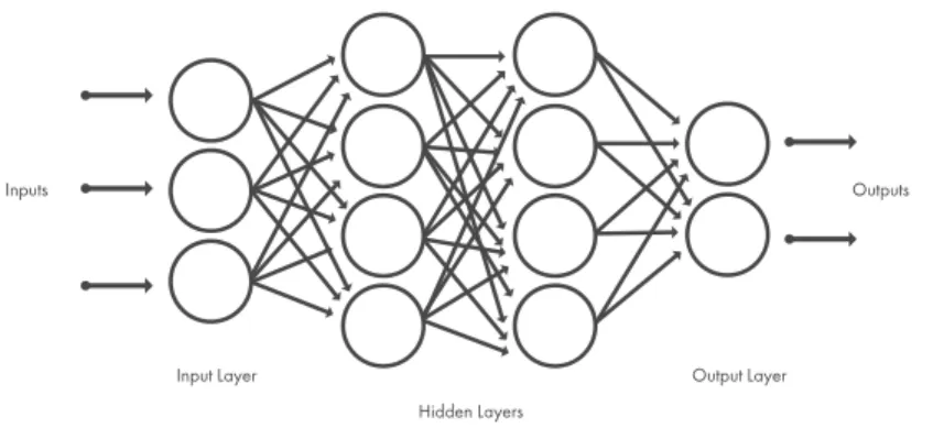
Figure 8. General neural network layout. ... 13

Figure 9. Neural Network layout obtained from MATLAB. ... 14

Figure 10. Left: example of drilling simulation (Von Mises stress). Right: nodal temperature of outer insert. 16 Figure 11. Test sample points. ... 17

Figure 12. Drill and workpiece assembly. From small to big diameter: d, C, D. ... 17

(7)

vi

Index of Tables Table 1. Number of elements and nodes resulting from meshing. ... 12

Table 2. Results from FE simulations. ... 18

Table 3. Results of the RMSE for each network in the cross validation. ... 20

Table 4. Comparison between results from simulations (left column) and from metamodel (right column). .. 22

Table 5. Tool material properties (AZoM, 2018). ... 27

Table 6. Workpiece general material properties (AZoM, 2018). ... 27

Table 7. AISI 1045 Johnson-Cook plasticity parameters (Nasr & Ammar, 2017). ... 28

Table 8. Ductile damage of workpiece (Nasr & Ammar, 2017). ... 28

(8)

Terminology

C

CAD

Computer Aided Design ... i, 3, 5, 7, 8, 10, 26 CNC

Computer Numerical Control ... 1

D

DIY

Do It Yourself ... 2

F

FEA

Finite Element Analysis ... 6 FEM

Finite Element Method ... i, 3, 5, 6, 7, 8, 9, 10, 26

M

MOOP

Multi-Objective Optimization Problem ... 7, 15 MRR

Material Removal Rate ... 7, 14, 18

N

NSGA-II

Non-Dominated Sorted Genetic Algorithm - 2nd version . 7, 15, 20

S

STEP

(9)

1

1 Introduction

Metalworking is the process of working with metal to create individual parts, assemblies, etc. Machining is a metal cutting process wherein material is taken to a specified geometry by removing excess of material. Drilling a hole in a metal body is one of the most common example. When using a drill, the temperature of the cutting tool rises significantly partly due to the friction between the surfaces of the drill and the workpiece, leading it to an early wear. In this thesis the behaviour of a drill head with replaceable inserts is going to be studied. These inserts are used to prolong the life of the tool while obtaining a better and smoother surface of the hole. However, these tools also suffer of wear and can produce a poor surface finish or a tolerance outside the normal range (Sandvik Coromant, 2018). The tool wear is usually produced by variables such as the speed and the feed. A study is needed to find out how these two parameters would have to be set to maximize the material removal rate while minimizing the wear to increase the tool life.

Therefore, simulations are required for this study. Simulations are virtual reproductions of the behaviour of any real process or system. The main issue with simulations is that these are computationally expensive, thus to explore more solutions without spending large amounts of time, a metamodel is needed. A metamodel is a simplified model of a system, or the actual model, which should be computationally cheaper.

1.1 Background

As stated by Collins Dictionary (Dictionary, 2018), “Drilling is the process of cutting holes in a solid

material using a rotating cutting tool.” Humans have discovered the benefits of using rotary tools

since the Upper Palaeolithic era (Singer, Holmyard, & Hall, 1967). Throughout the history, there have existed many types of drill, e.g. hand drills (Figure 1) (manually powered), pistol-grip drills (powered electrically), vertical drills or CNC drilling machines (controlled by a computer). They all have in common a rotary tool used to remove material from a solid body.

(10)

Figure 1: Example of an old hand drill.

Nowadays, there is an even much wider range of specific drills for each different task, whether is going to be used for DIY, for small workshops of mass production in the industry.

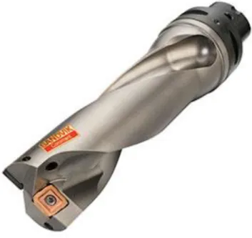
In this project, the drill head to be analysed is the Sandvik Coromant CoroDrill® 880 (Figure 2). This tool is commonly used in industry to drill holes in metallic bodies with a high accuracy and small hole tolerances (Coromant, 2018). This drill has two replaceable inserts; one located partly eccentric of the center of the cutting tool and the other one fully eccentric to the edge, to cut the inner section of the hole and the outer part, respectively.

(11)

3

1.2 Goals

The proposed approach will involve the use of a CAD software (Autodesk Inventor® Professional 2018), a FEM software (ABAQUS 6.14) for the simulations and a programming software for the optimization (MATLAB R2017B). A literature research is needed within metal cutting and specifically within drilling operations.

The aim of the project is to optimize a drilling process operation regarding its speed and feed, maximizing the material removal rate while minimizing the wear to increase its life. An algorithm has to be used in MATLAB and then integrate the code in the FEM software.

The objectives of this research project can be summarized as follows:

• Design and use of a 3D CAD model of a specific drilling tool with replaceable inserts. • Modelling and analysis using FEM.

• Metamodelling.

• Analysis of parameter sensitivity.

• Use learned skills to optimize speed and feed of this machining process.

The importance of this research is the capability to build a virtual model, make simulations and then optimize it without the use of physical equipment, therefore reducing costs while increasing the efficiency of the product.

The originality of this project is not just the simulation and optimization of a metal cutting process. There are existing studies regarding drilling (see literature review below, section 2.1), but none of them has used a drill head with replaceable inserts. These new type of drilling tools are made for precise metal cutting and at higher speeds than a common drill.

1.3 Limitations

There are no previous studies related to drills with replaceable inserts. The tool is made by Sandvik, which did not provide enough data for the design of the 3D model, so this had to be a simplified model which then would be exported to Abaqus in a STEP file, avoiding any geometry information loss in the FEM software.

(12)

However, the unavailability of huge amounts of training data for the neural network, could make the metamodel not accurate enough, eventhough there is only two parameters as input (feed and speed).

In regard to this project the biggest limitation is time, since the simulations are very computationally expensive. Also the process to achieve the results is very arbitratry andl every step is depending on the previous one, which limits the work.

The provided computers at the University of Skövde were not capable to run most of the simulations until the end, so the work was done on a personal computer.

(13)

5

2 Method

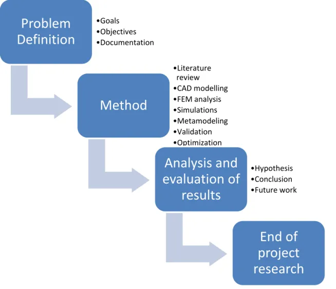
Within this chapter, the method followed for this research is explained. Figure 3 shows a process diagram including an overview of the different steps and methods in the order that is used. First, a literature review is required, focusing mainly in different case studies and experiments regarding drilling process. Then, the 3D-CAD model is designed, continuing with an analysis which will be made using FEM (finite element method), and last step is the metamodeling and its validation to measure the performance or the error of the metamodel.

Figure 3: Process diagram of the research project

Once the method is completed, the results would have to be analysed and try to draw a hypothesis or a generalizable theory within the changes on the main parameters regarding drilling.

Problem

Definition

•Goals •Objectives •Documentation

Method

•Literature review •CAD modelling •FEM analysis •Simulations •Metamodeling •Validation •Optimization

Analysis and

evaluation of

results

•Hypothesis •Conclusion •Future work

End of

project

research

(14)

2.1 Literature review

One of the main problems in metal cutting processes is the plastic deformations that produce heat in the workpiece when the material is being removed by the cutting tool. In addition, the tool wear is also caused by the heat generated when drilling the workpiece due to friction. This literature review is mainly focused on drilling simulations.

Tool wear has a big impact not only on the tool life but also on the quality of the finished product regarding its dimensional accuracy and surface roughness (Attanasio, Faini, & Outeiro, 2017). In their experiment, they analyse the phenomena that cause tool wear in a nickel-based alloy of a drilling tool depending on selected cutting parameters; cutting speed and feed rate. The FEM software SFTC DEFORM-3D FEA is used to simulate tool wear in drilling of Inconel 718 (Attanasio, Faini, & Outeiro, 2017). The followed routine focuses on calculating the amount of tool wear, then define the worn tool geometry to update the mesh. Therefore, the predicted flank wear distribution on the tool edges is compared with the simulation results (within different simulation times) to demonstrate the high accuracy of their procedure to capture the tool wear in drilling.

A study has been conducted within the effects of different levels of abstraction simulating heat sources in FEM within drilling process. There are three different types of abstract heat sources described in this paper among many different types (Bollig, Köhler, Zanger, & Schulze, 2016). The first one is to apply the heat boundary condition in a set of nodes in the surface of the hole. The second heat source model is based on conical segments with an interior angle of 130 degrees due to the drilling tool (Bollig, Köhler, Zanger, & Schulze, 2016). The third model uses the second model but in addition is circularly divided into 12 parts. According to Bollig et al. (2016), the different abstract heat sources have shown an important effect on the temperature distributions and phase transformation. The results show that the closest the approach to the drilling process (third model) the most realistic simulation results. This could be helpful at the time of modelling and meshing in the FEA of the current research project.

A paper presented by Isbilir and Ghassemieh (2011) study the drilling process through simulations by using ABAQUS. Their model simulates the drilling process regarding the damage initiation and evolution of the workpiece material rather than different heat scenarios. The results showed that the FE model of drilling is able to predicts changes in cutting force, torque and stresses respect to drilling process parameters.

(15)

7 There are also lots of papers related to optimization on machining processes where the MRR is to be maximized. To predict the output in electrochemical machining, the MATLAB Neural Network Toolbox was used (Kasdekara, Parashar, & Arya, 2018), by introducing four different input variables (voltage, feed rate, electrolyte concentration and conductive electrone) and one output of MRR. Kasdekara et al. (2018) emphasizes in the importance of validating to confirm that the training of the network is sufficient, otherwise the predictions would not be accurate. The use of neural networks permits finding optimal solutions to MOOP without executing a large number of FEM simulations, therefore avoiding these heavily computing system (D’Addona & DarioAntonelli, 2018).

As for the tool wear, it has been shown that the flank wear on tools is directly related to the nodal temperature (Rao, Nageswara Rao, & N Someswara Rao, 2006). The conducted study by Rao et al. (2006) investigated diffusion wear, occurring at high cutting speeds, on the tool for prediction of flank wear by using artificial neural networks.

However, to find the pareto front of all the non-dominated sample points containing their speed and feed, NSGA-II is a common and reliable technique used to solve multi-objective optimization problems of different machining processes and its performance (Yusoff, Salihin, Azlan, & MohdZain, 2011). The machining obejctives that are usually performed are tool wear, MRR or crater depth, and as process parameters, the depth of cut and cutting speed, among many others (Yusoff, Salihin, Azlan, & MohdZain, 2011).

These studies have in common the main parameters: feed rate[m/rev], cutting speed[m/s], time[s] and temperature[ºC]. Therefore, these would be the first variables to take into account when having to optimize the material removal rate and the wear, which are directly related to them.

However, none of the above papers covers any study related to a modular drill or cutting tools with inserts. Also, there is no research conducting to an understanding of how these new tools with replaceable bits would wear off by analysing the mentioned parameters using FE simulations.

2.2 Methodology

This research project is composed by the following main parts: CAD modelling, FEM analysis and simulations, metamodeling and optimization.

(16)

2.2.1 CAD modelling

Computer aided design (CAD) is the use of a wide range of computational tools that assist engineers, architects and designers in their work.

Within this project, the top section of the drill head and the inserts are drawn in a 3D-CAD software (Autodesk Inventor® Professional 2018) and will be exported to the FE software (ABAQUS) as STEP files. The 3D models are approximations of the Sandvik Coromant CoroDrill® 880 inserts and the dimensions are taken from the official webpage, and the missing ones are measured proportionally to the provided 2D drawing (Figure 4). These inserts have a chip breaker design optimized for accelerated chip evacuation as well as the roughness of the surface finish is small.

Figure 4: 2D Drawing and given dimensions of the drill inserts provided by Sandvik Coromant.

The below picture shows the result of the CAD drawing of the insert and the bottom part of the drill head assembly (Figure 5).

(17)

9

2.2.2 FEM analysis and simulations

The finite element analysis is a numerical technique to find approximate solutions for systems of partial differential equations, often used to solve problems in mechanics. It works by dividing the body that needs to be analysed into smaller objects called finite elements. The stresses in these elements then can be calculated using boundary conditions and applied loads. By calculating the stresses on all finite elements, a result for the entire system is achieved. The general steps to do a FEM are the following:

• Definition of geometry and materials: When choosing a material, the needed paremeters, such as the Young’s modulus or the yield strength, are defined (see Appendix B).

• Choice of type of analysis: Depending on the type of elements and its degrees of freedom (related to temperature and displacement). In this FEA a fully coupled thermal-displacement analysis in ABAQUS/Explicit is chosen, which is used specifically for a highly nonlinear process in which elements suffer of extreme deformation, allowing to handle computational expensive analyses.

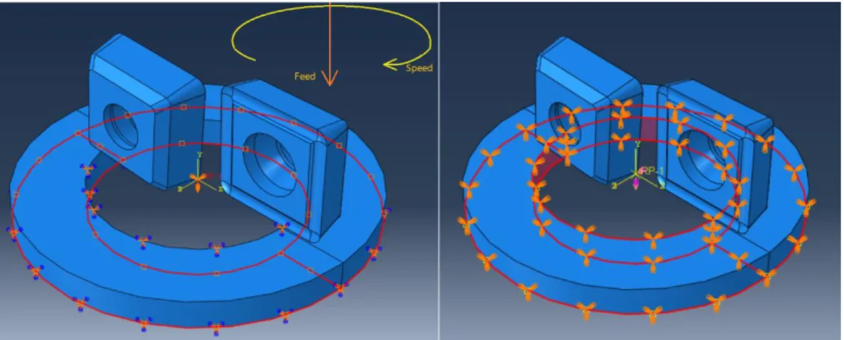
• Application of boundary conditions and loads: Boundary conditions represent connections to the environment. The loads are forces, pressures or moments on the part that is analysed, resulting from the system. These usually need to be calculated by hand and are inserted on edges, corners or faces in the model. This will also involve the drawing of the path that the drill will follow. The speed and feed are set in negative values in ABAQUS/Explicit so the drill would move down in the Y-axis and rotate clockwise in the XZ-plane. Figure 6 below shows (on the left) the reference point (RP-1), where the speed and feed are set, as well as their directions and the bottom surface of the workpiece being set at 20ºC, (on the right)and how the workpiece is fixed to the bottom and the inner surface so there would not be displacement of the part when cutting.

(18)

Figure 6. Boundary conditions.

• Definition of element type and size: Before dividing the body into smaller elements (meshing), the element type has to be defined relying on the part´s geometry and type of analysis. Therefore, the workpiece was assigned a hexaedric and the inserts tetraedric types of elements, both in the family of coupled temperature-displacement. The size of the elements will be crucial when obtaining results, meaning that if the elements are too big or disproportionate, the drill will not cut the workpiece properly, but the smallest the size, the better results in exchange for greater simulation times. Thus the approximate global size for the elements are set to 0.0002 meters (20 µm), which were found out to be small enough to cut the workpiece smoothly. A mesh convergence study is recommended for more accurate results. This could be done by trying different mesh size and applying the same and find at what mesh size the maximum stress converge to a stable value.

• Meshing: The parts are divided into finite elements. This task is often done automatically by the FE-software after choosing the shape of each element (see Figure 7 below).

• Solution: The problem is solved, calculating values for the deformation, von Mises stresses, safety factor, nodal and elements temperatures, etc. Since the current research involves the FEA of a whole machining process and not just a simple static analysis of a part, ABAQUS will also calculate other variables´ values such as the amount of removed material and its dimensions.

• Interpretation of solution: For example, the solution must be checked for peak strains that may result from problems with boundary conditions within the simulation that will not appear in an actual part. Obviously, the overall resulting stresses and deformations have to be checked, since these are the data that are needed.

(19)

11 This would be a general overview to proceed with the FEM. In this thesis, first step was to import the different parts of the drill from the CAD software to the FE software in STEP format. These STEP files save all the needed information about the geometry of the parts to make the final assembly. The material specifications and behaviour that are needed to make the drill simulation are conductivity, density, elasticity, plasticity and specific heat for both the drill and the workpiece. In addition, ductile damage and shear damage are added to the workpiece.

Figure 7. Final model before and after meshing.

Now that the model characteristics are set, contact interaction between the cutting edges of tboth the inner and outer inserts and the surface of the workpiece are defined, as well as the convection (Surface film condition) is defined according to the material and a sink temperature of 20ºC.

For the contact property, additional friction coefficient is set at 0.3 due to the tangential behaviour of this material of the drill on the workpiece according to given data.

Nevertheless, boundary conditions of the actual drilling process are defined. These are the workpiece being fixed, its initial temperature, and the speed and feed of the drill during the machining procedure. The values of speed and feed would eventually be changed to various different values to obtain different results that this experiment is seeking for.

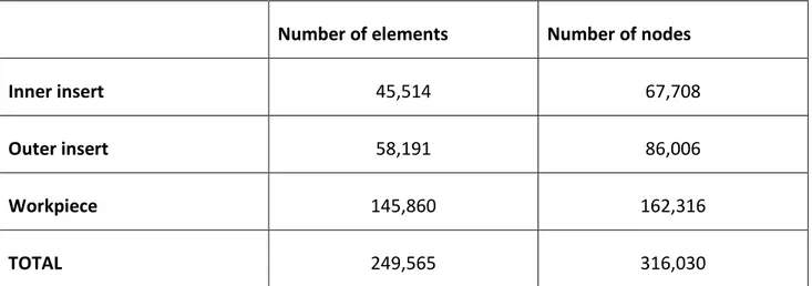
For the workpiece the elements are hexaedrical and tethrahedrons for the inserts (Figure 7). The below table (Table 1) shows the number of elements and nodes obtained by the meshing tool in Abaqus:

(20)

Table 1. Number of elements and nodes resulting from meshing.

Number of elements Number of nodes

Inner insert 45,514 67,708

Outer insert 58,191 86,006

Workpiece 145,860 162,316

TOTAL 249,565 316,030

The drill attachement was also divided in 1348 elements and 2414 nodes, but since this part is irrelevant for the FE analysis, it was suppressed from the simulation.

However, the ouput requested data includes stresses, forces, displacements, velocity, failure and temperatures are needed to get the necessary results from the simulations.

In this research, the model aims to simulate the drilling process, repeating it with different values of speed and feed to obtain the best results to extend the life of the tool. This will be done in the optimization part.

2.2.3 Simulations and metamodeling

Before running the first simulations to build the metamodel, a set of data points have to be created so the metamodel would fit adequately over the whole design space. These data points are the design of experiment. There are different types of methods to create these points like Monte Carlo (MC) or Latin Hypercube (LHC) samplings. They both are used to generate random samples of X points for each pair of input variables (in this multi-objective problem), with the difference that the LHC sampling creates more uniform and spread points (Vose, 2014). Because of lack of time and uncertainty of how many simulations are to be run, the function rand() in MATLAB, which returns uniformly distributed random numbers (MATLAB, 2018), is used.

Once the sample points are all created, the metamodel will be created by using the MATLAB Neural Network fitting toolbox. A neural network is a computing model that works in a similar way than the neurons in the human brain. Neural networks are used to perform pattern recognition combining several hiding layers, using only simple operations in parallel in every hidden layer. There is an input

(21)

13 layer that is connected to the hidden layer, or layers, via nodes (called neurons) and these to the output layer (Figure 8).

Figure 8. General neural network layout.

Therefore, the sample points from the simulations and the results are to be the input and output of the neural network, respectively.

The performance and accuracy of the metamodel will depend on the number of samples and their quality (Amouzgar, 2018). A validation has to be carried out to measure its performance, so a popular and cheap computing validation method is the k-fold cross validation (Amouzgar, 2018). This statistical method used in machine learning to predict the performance of the metamodel. The general procedure is:

1. Original k sample points of a set are saved.

2. Substract a single sample and retain it for validation. 3. Rest k-1 samples are used as training data.

4. Repeat previous steps k times.

5. Calculate average of the k results for a single final result.

The k-fold cross validation method is suitable for this thesis since all the points are used as training and validation data without leaving any sample out.

Training a neural network requires input data and the output to recognize a pattern and therefore obtain restuls in a simplified model of the simulation or metamodel. MATLAB Neural Network toolbox has been used to create the neural network. The input (cutting speed and feed) and output (nodal temperature) are imported from a text file. Then the size of the hidden layers of 10 is chosen following the following rule of thumb (1) (Esmaili, 2015):

(22)

𝑠𝑎𝑚𝑝𝑙𝑒𝑠_𝑠𝑖𝑧𝑒 ≥ ℎ𝑖𝑑𝑑𝑒𝑛_𝑙𝑎𝑦𝑒𝑟_𝑠𝑖𝑧𝑒 × (𝑖𝑛𝑝𝑢𝑡_𝑠𝑖𝑧𝑒 + 𝑜𝑢𝑡𝑝𝑢𝑡_𝑠𝑖𝑧𝑒) (1) 35 ≥ ℎ𝑙𝑠𝑖𝑧𝑒 × (2 + 1)

ℎ𝑙𝑠𝑖𝑧𝑒 ≤35 3

MATLAB offers three training functions for its Neural Network toolbox: • Levenberg-Marquardt 'trainlm' is usually fastest.

• Bayesian Regularization 'trainbr' takes longer but may be better for challenging problems. • Scaled Conjugate Gradient 'trainscg' uses less memory, being suitable in low memory

situations.

Levenver-Marquardt is used for this training sample, obtaining the following neural network (Figure 9):

Figure 9. Neural Network layout obtained from MATLAB.

2.2.4 Validation

For the validation, k-fold cross validation (explained earlier in section 2.2.3) is carried out. The MATLAB neural network performance function perform(net, t, y) calculates automatically the mean squared error (MSE):

𝑀𝑆𝐸 =1

𝑛∑ (𝑌𝑖 − 𝑌̂𝑖) 2

𝑖 (2)

𝑅𝑀𝑆𝐸 = √MSE (3)

Where n is the number of points, 𝑌𝑖 is each testing point from the simulation and 𝑌̂𝑖 is each result from the metamodel.

(23)

15 But the root mean squared error (RMSE) is a directly interpretable results rather than the MSE, since it has the same units as the output.

Therefore, the cross validation and the MATLAB neural network have been combined in a script where the data is imported and normalized, and then put into a loop to train the samples 35 times, obtaining 35 networks where one data is saved for validation. The MATLAB script running the cross validation is shown in the Appendix C.

2.2.5 Optimization

This part is to use an algorithm in a programming software (MATLAB 2017a) using all the steps registered by ABAQUS. This FE software creates an input file (.inp) with all the necessary data to make the FEA, and saves all the steps followed by the software to do the simulation in python script files (.rpy). This will be used and exported to MATLAB code and integrate it with the algorithm to repeat the simulation repeated times with different variables´ values until specific feed and speed are found to reduce the wear and increase the material removal rate (MRR). These two are the parameters to optimize; minimizing and maximizing respectively.

𝑓(𝑥) = {𝑀𝑖𝑛𝑖𝑚𝑖𝑧𝑒 𝑡𝑜𝑜𝑙 𝑡𝑒𝑚𝑝𝑒𝑟𝑎𝑡𝑢𝑟𝑒 𝑀𝑎𝑥𝑖𝑚𝑖𝑧𝑒 𝑀𝑅𝑅

In multi-objective optimization problems, Non-Dominated Sorting Genetic Algorithm (NSGA-II) (Deb, Pratap, Agarwal, & Meyarivan, 2002) and Strength Pareto Evolutionary Algorithm (SPEA2) (Zitzler, Laumanns, & Thiele, 2001) are two of the most commonly used, and showing better results in general compared to other algorithms (Amouzgar, 2018). It has been found that the non-dominated solutions obtained by SPEA2 are better than NSGA-II in terms of convergence and diversity (the solutions that are closer to the pareto optimal front and the diversity of these solutions), but at the same time is computationally more expensive (King, Deb, & Rughooputh, 2010). Since the present MOOP has only two objectives, and time is a big matter, NSGA-II is chosen.

(24)

3 Results

The results of the thesis are presented in this section, consisting on the results from the FE simulations, metamodeling and optimization.

3.1 Finite element simulations and sampling

Cutting speeds used in these Sandvik insert drills are up to 400 to 600 mm/s, and feed around 0.004 to 0.006 mm/rev. The problem with these velocities is that the simulations’ run are extremely long, so instead these values have been increased to 1500 to 2500 for speed, and 0.35 to 0.6 for feed. The problem is by running simulations at extremely high speeds is that the tool temperature will probably raise considerably and results would not be realistic. The step time is set 0.002 seconds, being this the minimum time that the simulation takes so the temperature increase stabilizes. A better way to obtain more accurate results could be running the simulation for around 1 second with the actual speeds. This is the main reason for why this thesis will be more as a framework for future work. In high speed machining, when the chip-tool interface temperature is very high to start mass transfer, results in wear by diffusion, which significantly contributes to the tool life (Ghosh & Bhattacharyya, 1968). Therefore, the first simulation is run in different trial speeds, it has been noted that the highest temperature in the drill comes from the outer insert. The nodes with the highest temperatures are located where the outer insert of the tool cuts the inner part of the workpiece (Figure 10), so this is the part to be more analysed at the highest velocity.

(25)

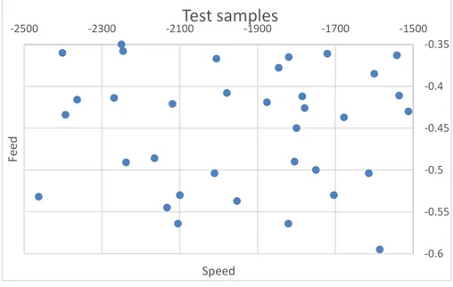
17 Nevertheless, input files have to be set with the different speeds before executing the command. The random numbers that have been generated by the rand() function in MATLAB have been plot in a graph (Figure 11). A total of 35 points have been generated for the simulations (larger sample points would give more accurate results).

Every sample point consist in a cutting speed and a feed values, and an input file has been created for each one of them from a general input file containing all the information to run the simulation.

Figure 11. Test sample points.

The material removal rate depends on the tool geometry, feed, speed and depth of cut. This is calculated in excel since it is a straightforward calculus. The needed equations are the next:

𝐴 = (𝐶 − 𝑑) ∙ 𝑓 𝐴 = (12 − 9) ∙ 𝑓

𝑀𝑅𝑅 = 𝑣 ∙ 𝑓 ∙ 3

Where d is the inner diameter of the workpiece, C the diameter of the drill, v is the speed, f is the feed and A is the total cutting area of the drill.

Figure 12. Drill and workpiece assembly. From small to big diameter: d, C, D.

-0.6 -0.55 -0.5 -0.45 -0.4 -0.35 -2500 -2300 -2100 -1900 -1700 -1500 Fe ed Speed

Test samples

(26)

The nodal temperature is calculated by ABAQUS during the simulations.

The results of each simulation are shown below in Table 2. The table contains the sample points, the depth of cut, the MRR and the nodal temperature obtained from every simulation.

Table 2. Results from FE simulations.

Simulation Speed [mm/s] Feed [mm/rev] Depth of cut [mm] MRR [mm3_{/s] NT [ºC]} 1 -1536 -0.411 3.3490504 1893.888 17419.1 2 -1953 -0.537 5.56371883 3146.283 55948.6 3 -1979 -0.408 4.28345889 2422.296 21277.6 4 -2269 -0.414 4.98337401 2818.098 23061.5 5 -2011 -0.504 5.37689125 3040.632 48908.2 6 -1876 -0.419 4.1699947 2358.132 18596.7 7 -1821 -0.564 5.44850928 3081.132 60664.5 8 -2105 -0.564 6.29824934 3561.66 84707.5 9 -2133 -0.545 6.16702918 3487.455 69119.4 10 -1512 -0.43 3.44912467 1950.48 17197.4 11 -2463 -0.532 6.95127852 3930.948 79585.7 12 -1614 -0.504 4.31541645 2440.368 17886.5 13 -1586 -0.595 5.0062069 2831.01 42481.7 14 -1704 -0.53 4.79108753 2709.36 35699 15 -2402 -0.36 4.58737401 2594.16 24657.9 16 -2238 -0.491 5.82948541 3296.574 40673.1 17 -2165 -0.486 5.58190981 3156.57 46355.1 18 -1820 -0.365 3.52413793 1992.9 18272 19 -2364 -0.416 5.21710345 2950.272 25341.1 20 -1779 -0.426 4.02044562 2273.562 19236.4 21 -2394 -0.434 5.51191512 3116.988 34248.3 22 -1846 -0.378 3.7017931 2093.364 18157.2 23 -2006 -0.367 3.9055809 2208.606 20711.2 24 -1721 -0.361 3.29592042 1863.843 19228.2 25 -1785 -0.412 3.90143236 2206.26 20941.9 26 -1542 -0.363 2.9694748 1679.238 14399.5 27 -1678 -0.437 3.89011141 2199.858 17519.1 28 -1805 -0.49 4.69204244 2653.35 21164.5 29 -2246 -0.358 4.26561273 2412.204 24163.2 30 -2119 -0.421 4.73262069 2676.297 21483 31 -1750 -0.5 4.64190981 2625 19656.1 32 -2250 -0.35 4.17771883 2362.5 21133.1 33 -1800 -0.45 4.29708223 2430 19508.9 34 -2100 -0.53 5.90450928 3339 64319 35 -1600 -0.385 3.26790451 1848 17963.9

As it can be observed in the above table, the temperatures obtained by running the simulations are unrealisticly high due to the high velocities.

(27)

19

Figure 13. Plots of speed, feed and depth of cut with respect of nodal temperature.

As can be observed in the above graphs (Figure 13), it is difficult to identify a clear trend for the speed graph, but regarding the feed with respect to the nodal temperature, the higher the feed (in absolute values, negative sign shows the direction), thus the depth of cut, the higher the temperature. It is possible to say that the feed has a major impact in the tool wear than the speed.

3.2 Metamodel and validation

The metamodel built from the sample points and the resulting temperatures from the simulations gave an average network error, based on the RMSE (see section 2.2.3), of around 0.71% after running the script. This percentage is obtained by dividing the average RMSE by the mean of the temperatures obtained in the simulations. But comparing the results from the networks with the simulations, it is clear that the singular errors are bigger than the average. This can be due to the low number of sample points and also due to the fact that the final temperatures from the simulations are not realistic, and these numbers are around 150 times higher than common machining. The table below (Table 3) shows the RMSE from every fold form the cross validation.

(28)

Table 3. Results of the RMSE for each network in the cross validation.

RMSE for every fold [ºC]

RMSE for every fold [%] 9.08E-12 4.30E-14 3.81E-11 1.80E-13 57.83272874 0.2737 1.85E+02 0.8743 4.89E+02 2.316 3.292164238 0.0156 7.01E-11 3.32E-13 185.0742015 0.8758 5.56E+02 2.6326 3.67E+02 1.7343 9.36E-12 4.43E-14 4.74E-11 2.24E-13 379.2915965 1.7948 4.58E-11 2.17E-13 1.52E-11 7.21E-14 4.43E-11 2.10E-13 33.52551081 0.1586 47.46043615 0.2246 2.79E-11 1.32E-13 152.1207079 0.7198 1.33E+02 0.6281 467.4692972 2.212 2.00E+02 0.9465 179.1088649 0.8475 2.47E+01 0.1168 1.40E-11 6.62E-14 1.71E-11 8.11E-14 3.05E+01 0.1443 1.15E-11 5.45E-14 2.37E-11 1.12E-13 132.325721 0.6262 3.08E-11 1.46E-13 250.8411287 1.187 718.250912 3.3987 1.01E-11 4.76E-14

Regarding optimisation, it has been considered pointless to use any of the earlier mentioned algorithms (NSGA-II and SPEA2), since the objective of it is to obtain realistic results to improve the current machining process. The results will be discussed in the following section.

(29)

21

4 Discussion

The CAD model was a simple step but important to build the FE model. With the provided information from the manufacturer, the 3D model was easily made using Autodesk Inventor and then imported in STEP files to ABAQUS. The information shared in this type of files is not extensive, but sufficient to proceed with the FE model. However, it would have been ideal to get more accurate details from the inserts and a physical one.

Nonetheless, regarding the ABAQUS model, temperature condition and convection from the air was added, however no lubricant has been set for the simulations. This, together with setting a smaller global element size for the meshing, would have likely reduced the temperatures considerably, without downplaying the greater impact resulting from the high speeds.

The sample points, created using MATLAB function rand() (uniformly distributed random numbers generator). Using Latin Hypercube sampling would suit this problem better, although the points seem to be rather uniform (Figure 11), but another factor to consider is the number of test sample points. A higher number of sample points could allow to obtain an accurate metamodel. The number of sample points is indeterminable. It is known that is enough when the results of both converge, but this number can be reduced if the new sample points are chosen near the ones that did not give a good result.

Despite the fact that all these simulations are very computationally demanding and time consuming, running them at normal speeds would be possible in shorter periods of time using high-performance computing (HPC) clusters. These are servers were all the computing can be run, thus speeding up the time for the FEA.

However while metamodeling, eventhough the data is no realistic and probably insufficient, the Neural Network resulted in a better behaviour than expected. This does not mean that is perfect, but the k-fold cross validation showed a high accuracy performance for the Neural Network. It is observed that some values predicted by the metamodel were negative (Table 4). This results in a better performance since it is calculating the mean value from all the temperatures obtained.

(30)

Table 4. Comparison between results from simulations (left column) and from metamodel (right column). Nodal temperature from simulations [ºC] Nodal temperature from metamodel [ºC] 17963.9 16974.1 64319 43414.5 19508.9 23858.6 21133.1 30478.8 19656.1 56013.4 21483 24261 24163.2 43216.3 21164.5 43728.5 17519.1 79402.9 14399.5 40960.8 20941.9 40205.7 19228.2 119832.1 20711.2 24780.7 18157.2 19871.8 34248.3 5661.2 19236.4 84879.4 25341.1 56194.4 18272 25360.9 46355.1 17832.1 40673.1 18944.7 24657.9 -3283.5 35699 18028.1 42481.7 -11165.9 17886.5 14702.5 79585.7 20429.2 17197.4 15339.3 69119.4 22955.5 84707.5 8674.7 60664.5 20893.7 18596.7 61850.3 48908.2 20423.1 23061.5 22821.3 21277.6 17806.8 55948.6 57302.8 17419.1 22554.1

As seen above, comparing the results one by one, there seems to be a big difference, so the error can not rely from the mean temperatures, but from the average error.

(31)

23

5 Conclusion

This report includes all the steps followed to achieve a metamodel that can be used in the future for optimization applications of drilling simulations.

The CAD results and the FE model got satisfactory results, besides from the high speeds given. It is clear that increasing the speed or the feed can rise the nodal temperature, as well as the MRR. This can be easily changed from the input files and running longer simulations. A smaller mesh size and adding the appropriate lubricant to the drill will give more accurate results.

Also, it has been concluded that higher speeds and feeds are directly related to the temperature to increase, being the feed much more meaningful than speed (see Table 1). This is very relevant since the focus should be on finding a shorter range for the feed, where the temperatures would not increase unreasonably.

To continue this work starting from the FE model, would be convenient to automate the whole process. A pseudo-code could be:

Create 50 test points (at least) using Latin Hypercube sampling method. 1. Open and read input file.

2. Find cutting speed (VR2) and feed (V2) .

3. Give different values obtained from the LHC sampling. 4. Run the simulations and save results.

5. Use the script given in section 3.2 to create metamodel with the input data from sampling and the output obtained from the simulations and to validate the network.

6. Use NSGA-II (recommended) to obtain the optimal results from maximizing MRR and minimizing the nodal temperature.

The work presented in this thesis is a framework to use for future researches related to machining processes, metamodeling and optimization. Simulation´s input and output files can be requested to a16samak@student.his.se .

(32)

6 References

Amouzgar, K. (2018). Metamodel Based Multi-Objective Opitmization with Finite-Element

Applications. Skövde: University of Skövde.

Attanasio, A., Faini, F., & Outeiro, J. (2017). FEM Simulation of Tool Wear in Drilling. Procedia

CIRP, 58, 440-444.

AZoM. (2018). Azo Materials. Retrieved January 2018, from

https://www.azom.com/article.aspx?ArticleID=9153

Bollig, P., Köhler, D., Zanger, F., & Schulze, V. (2016). Effects of Different Levels of Abstraction Simulating Heat Sources in FEM Considering Drilling. Procedia CIRP, 46, 115-118.

Business Dictionary. (2018). Retrieved from WebFinance Inc.: http://www.businessdictionary.com/definition/product-development.html

Coromant, S. (2018). Sandvik.coromant.com. Retrieved March 16, 2018, from https://www.sandvik.coromant.com/en-us/products/corodrill_880

D’Addona, D. M., & DarioAntonelli. (2018). Neural Network Multiobjective Optimization of Hot Forging. Procedia CIRP, 67, 498-503.

Deb, K., Pratap, A., Agarwal, S., & Meyarivan, T. (2002, April). A fast and elitist multiobjective genetic algorithm: NSGA-II. IEEE Transactions on Evolutionary Computation, 6(2), 182-197. doi:10.1109/4235.996017

Dictionary, C. E. (2018). Collinsdictionary.com. Retrieved March 16, 2018, from

https://www.collinsdictionary.com/dictionary/english/drilling

Esmaili, I. (2015). ResearchGate. Retrieved January 13, 2019, from https://www.researchgate.net/post/What_is_the_best_number_of_neurons_in_a_hidden_layer _in_Neural_Network_Training_Toolbox_in_Matlab

Ghosh, A., & Bhattacharyya, A. (1968, January). Diffusion Wear of Cutting Tools. Annals of the

C.I.R.P., XVI, 369-375. Retrieved from https://www.researchgate.net/publication/282292907_Diffusion_wear_of_cutting_tools

(33)

25 Kasdekara, D. K., Parashar, V., & Arya, C. (2018). Artificial neural network models for the prediction

of MRR in Electro-chemical machining. Materials Today: Proceedings, 5, 772-779.

King, R. T., Deb, K., & Rughooputh, H. C. (2010). Comparison of NSGA-II and SPEA2 on the Multiobjective Environmentl/Economic Dispatch Problem. University of Mauritius Research

Journal, 16, 1-27.

MATLAB. (2018). Retrieved november 2018, from https://mathworks.com/help/matlab/ref/rand.html

Nasr, M. N., & Ammar, M. M. (2017). An evaluation of different damage models when simulating the cutting. Procedia CIRP, 58(16), 134-139.

Rao, C., Nageswara Rao, D., & N Someswara Rao, R. (2006, December). Online prediction of diffusion wear on the flank through tool tip temperature in turning using artificial neural networks. Proceedings of The Institution of Mechanical Engineers Part B-journal of

Engineering Manufacture, 220, 2069-2076.

Singer, C., Holmyard, E., & Hall, A. (1967). From Early Times to Fall of Ancient Empires. A History

of Technology, 1, 188.

Vose, D. (2014, July 8). liprof. Retrieved January 7, 2019, from http://liprof.com/blog/the-pros-and-cons-of-latin-hypercube-sampling

Yusoff, Y., Salihin, M., Azlan, N., & MohdZain. (2011). Overview of NSGA-II for Optimizing Machining Process Parameters. Procedia Engineering, 15, 3978-3983.

Zitzler, E., Laumanns, M., & Thiele, L. (2001). SPEA2: Improving the Strength Pareto Evolutionary Algorithm. 103, 1-21.

(34)

Appendix A: Predicted Time Plan

Activity W3 W4 W5 W6 W7 W8 W9 W10 W11 W12 W13 W14 W15 W16 W17 W18 W19 W20 W21 W22

Thesis specification 26/1

Literature review

Data gathering and analysis

CAD modelling

Integration of CAD model with the FEM software

FEM analysis / Simulation

Midterm presentation 12/3 Optimization Integration of optimization with simulation Report Final presentation

(35)

27

Appendix B: Material´s properties

a. Tool material properties

Table 5. Tool material properties (AZoM, 2018).

Conductivity 51.9 W/(mºC) Density 7820 Kg/m3 Elastic Young´s Modulus 200000000000 Pa Poisson´s Ratio 0.29 Specific Heat 432.6 J/(kgºC)

b. Workpiece material properties

Table 6. Workpiece general material properties (AZoM, 2018).

Conductivity 51.9 W/(mºC)

Density 7820 Kg/m3

Elastic Young´s Modulus 200000000000 Pa

Poisson´s Ratio 0.29

Inelastic Heat Fraction 0.9

(36)

Table 7. AISI 1045 Johnson-Cook plasticity parameters (Nasr & Ammar, 2017). PLASTIC (Johnson-Cook) A B C n m Melting Temperature Transition Temperature 1 553000000 600000000 0.0134 0.001 0.234 1 1460ºC 20ºC