ADOLESCENT SLEEP AND THE CIRCADIAN
PACEMAKER
by Nora Stack
A thesis submitted to the Faculty and the Board of Trustees of the Colorado School of Mines in partial fulfillment of the requirements for the degree of Master of Science (Applied Mathematics and Statistics).
Golden, Colorado Date
Signed:
Nora Stack
Signed:
Dr. Cecilia Diniz Behn Thesis Advisor
Golden, Colorado Date
Signed:
Dr. Greg Fasshauer Professor and Head Department of Applied Mathematics & Statistics
ABSTRACT
Adolescence is a critical time of social, physical, and mental development. Adolescents often exhibit a circadian phase delay in which they tend to go to bed later and wake up later compared to adults. This thesis seeks to understand the adolescent phase delay and its relationship to the circadian pacemaker, the body’s master clock. Using a dynamic circadian pacemaker model, we identify parameters that affect features of the circadian system that may contribute to the phase delay. Specifically, we focus on the effect of light on the phase and amplitude of the circadian pacemaker as model parameters are varied. We compare simulation results with data characterizing the adolescent clock under different weekend sleep protocols. This work has implications for understanding the mechanisms associated with the adolescent phase delay and may inform efforts to create schedules for adolescents that mitigate sleep loss and the resulting impacts on physical and cognitive performance.
TABLE OF CONTENTS
ABSTRACT ... iii
LIST OF FIGURES...v
LIST OF TABLES...xii
LIST OF SYMBOLS ...xiv
ACKNOWLEDGMENTS ...xvi
DEDICATION...xvii
CHAPTER 1 MOTIVATION ...1
CHAPTER 2 BACKGROUND ...2
CHAPTER 3 CIRCADIAN PACEMAKER MODEL ...4
CHAPTER 4 PHASE RESPONSE CURVES AND AMPLITUDE RESPONSE CURVES ...7
CHAPTER 5 CROWLEY AND CARSKADON DATA...19
CHAPTER 6 SIMULATING INDIVIDUAL CASES ...27
CHAPTER 7 FUTURE DIRECTIONS ...39
LIST OF FIGURES
Figure 3.1 Behavior of the circadian pacemaker elements x and xc with a light
protocol of 500 lux from 8:00-0:00 and 0 lux from 0:00 to 8:00. The parameter values used for this simulation are the original (adult) model parameters...6 Figure 4.1 One cycle light protocol from Jewett et al. After a 40 hour constant
routine where phase is assessed, the participant is in 0 lux for 8 hours. They are then in 150 lux for 5.1 hours. For 0.3 hours, the light
transitions to bright light (2488 lux for 0.1 hrs, 4825 lux for 0.1 hours, and 7162 lux for 0.1 hours) and bright light at 9500 lux is maintained for 4.6 hours. The light transitions through lower light intensities for 0.3 hours (7162 lux for 0.1 hours,4825 lux for 0.1 hours, and 2488 lux for 0.1 hrs). The participant then experiences 5.1 hours at 150 lux and 8 hours at 0 lux. Phase is assessed a second time following the
completion of this cycle...8 Figure 4.2 Two cycle light protocol from Jewett et al. After a 40 hour constant
routine where phase is assessed, the participant is in 0 lux for 8 hours. They are then in 150 lux for 4.9 hours. For 0.3 hours, the light
transitions to bright light (2488 lux for 0.1 hrs, 4825 lux for 0.1 hours, and 7162 lux for 0.1 hours)and bright light at 9500 lux is maintained for 5 hours. The light transitions through lower light intensities for 0.3 hours (7162 lux for 0.1 hours,4825 lux for 0.1 hours, and 2488 lux for 0.1 hrs). The participant then experiences 4.9 hours at 150 lux and 8 hours at 0 lux. The light protocol is then repeated again. Phase is
assessed a second time following the completion of the second cycle. ...8 Figure 4.3 One Cycle PRC varying s2. The x-axis is the Initial Phase where an
Initial Phase = 0 corresponds to CBTmin. The y-axis is phase shift in
hours. Negative phase shifts indicate phase delays and positive phase shifts indicate phase advance. With increasing values of s2, the general
behavior of the adult model is maintained, but regions of phase advance decrease while regions of phase delay increase. ...10 Figure 4.4 Minimum Phase Shift from One Cycle PRC varying s2. The x-axis is
the range of values for parameter s2. The left y-axis is the minimum
phase shift and the right axis is the Initial Phase of the minimum phase shift. With increasing values of s2, the minimum phase shift (blue)
Figure 4.5 Maximum Phase Shift from One Cycle PRC varying s2. The x-axis is
the range of values for parameter s2. The left y-axis is the maximum
phase shift and the right axis is the Initial Phase of the maximum phase shift. With increasing values of s2, the maximum phase shift
(blue) decreases and the Initial Phase of the maximum phase shift
(orange) occurs later relative to CBTmin. ...12
Figure 4.6 Two Cycle ARC varying s2. The x-axis is the Initial Phase where
Initial Phase = 0 = CBTmin. The y-axis is Final Amplitude (F A)
which is percent initial amplitude. With increasing values of s2 the
minimum final amplitude decreases and then begins to increase. While the Initial Phase of the minimum final amplitude increases with
increasing s2 values. The general behavior of the adult ARC is
maintained with changes to s2 values...13
Figure 4.7 Minimum final amplitude analysis from the Two Cycle ARC varying s2.
The x-axis is the range of values for parameter s2. The left y-axis is the
minimum F A and the right axis is the Initial Phase of the minimum F A. With increasing s2 values minimum F As (blue) create an almost
parabolic shape, meaning that with increasing s2 values minimum F A
decreases and then begins to increase. The Initial Phase of the
minimum F A (orange) increases as s2 gets larger... 13
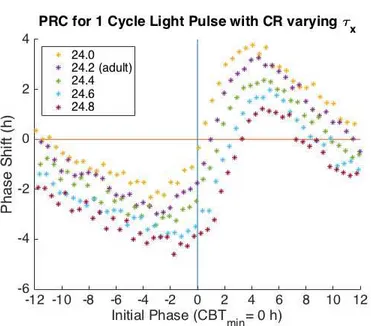
Figure 4.8 One Cycle PRC varying τx. The x-axis is the Initial Phase where an
Initial Phase = 0 corresponds to CBTmin. The y-axis is phase shift in
hours. Negative phase shifts indicate phase delays and positive phase shifts indicate phase advance. With increasing values of τx regions of
phase advance decrease while regions of phase delay increase while
maintaining the general behavior of the adult model...14 Figure 4.9 Minimum Phase Shift from One Cycle PRC varying τx. The x-axis is
the range of values for parameter τx. The left y-axis is the minimum
phase shift and the right axis is the Initial Phase of the minimum phase shift. Larger τx values produce decreases in the minimum phase shift
(blue) while the Initial Phase of the minimum phase shift (orange)
shifts later to CBTmin. ...14
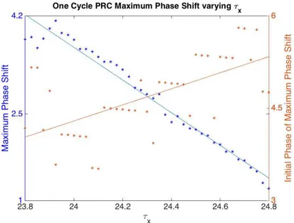
Figure 4.10 Maximum Phase Shift from One Cycle PRC varying τx. The x-axis is
the range of values for parameter τx. The left y-axis is the maximum
Figure 4.11 Two Cycle ARC varying τx. The x-axis is the Initial Phase where
Initial Phase = 0 = CBTmin. The y-axis is Final Amplitude (F A)
which is percent initial amplitude. With increasing values of τx the
minimum final amplitude increases and the Initial Phase of the min F A also increases. The general behavior of the adult ARC is maintained
with changes to τx values. ...15
Figure 4.12 Minimum final amplitude from Two Cycle ARC varying τx. The x-axis
is the range of values for parameter τx. The left y-axis is the minimum
F Aand the right axis is the Initial Phase of the minimum F A. With increasing τx values, the minimum F A (blue) increases. The Initial
Phase of the minimum F A (orange) increases as τx increases. ...16
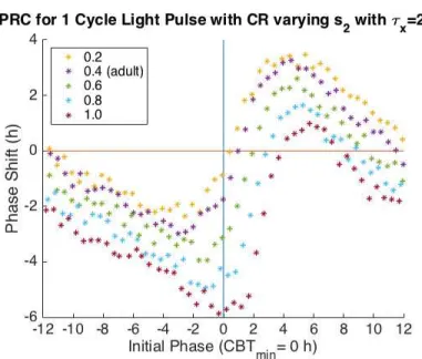
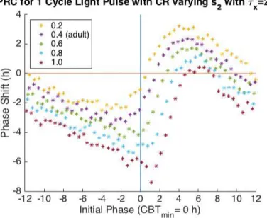
Figure 4.13 One Cycle PRC varying s2 with τx = 24.4. The x-axis is the Initial
Phase where an Initial Phase = 0 corresponds to CBTmin. The y-axis is
phase shift in hours. Negative phase shifts indicate phase delays and positive phase shifts indicate phase advance. Increasing the value of s2
while τx = 24.4 produces smaller regions of phase advance and larger
regions of phase delay while maintaining the general behavior of the
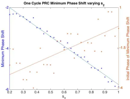
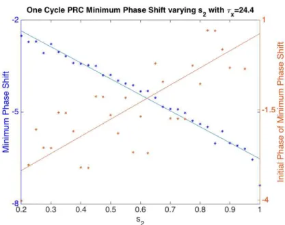
adult model. ...16 Figure 4.14 Minimum Phase Shift from One Cycle PRC, varying s2 with τx = 24.4.
The x-axis is the range of values for parameter s2. The left y-axis is the
minimum phase shift and the right axis is the Initial Phase of the minimum phase shift. Larger values of s2 decrease the minimum phase
shift (blue) and shifts the Initial Phase of the minimum phase shift
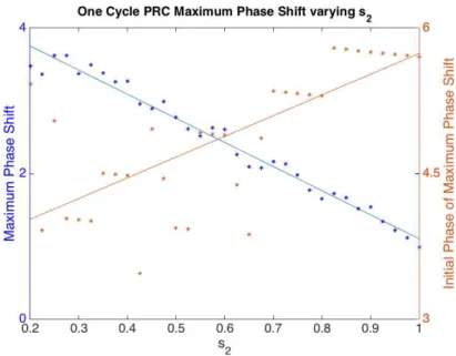
(orange) to later in the day. ...17 Figure 4.15 Maximum Phase Shift from One Cycle PRC, varying s2 with τx = 24.4.
The x-axis is the range of values for parameter s2. The left y-axis is the
maximum phase shift and the right axis is the Initial Phase of the maximum phase shift. The maximum phase shift (blue) decreases with larger s2 values. The Initial Phase of the maximum phase shift (orange)
occurs later relative to CBTmin as s2 increases...17
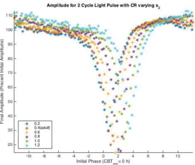
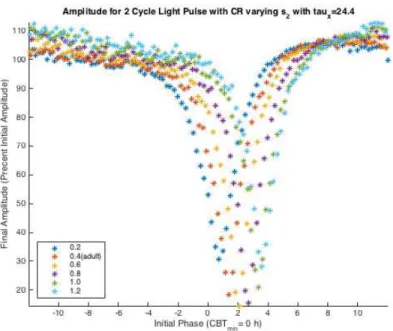
Figure 4.16 Two Cycle Amplitude, varying s2 with τx = 24.4. The x-axis is the
Initial Phase where Initial Phase = 0 = CBTmin. The y-axis is Final
Amplitude (F A) which is percent initial amplitude. With increasing values of s2 the minimum final amplitude decreases and then begins to
increase. While the Initial Phase of the minimum final amplitude increases with increasing s2 values. The general behavior of the adult
Figure 4.17 Minimum final amplitude analysis from Two Cycle ARC varying s2
with τx = 24.4. The x-axis is the range of values for parameter s2. The
left y-axis is the minimum F A and the right axis is the Initial Phase of the minimum F A. With increasing s2 values, the minimum F A (blue)
decreases and then begins to increase. The Initial Phase of the
minimum F A (orange) increases as s2 increases. ...18
Figure 5.1 The TYPICAL protocol. Time is plotted relative to the weekday bedtime (0=23:00).Yellow represents periods of wake, blue is sleep, green is dim light conditions for saliva collections in the lab, and grey is the transportation time between the lab and home. ...19 Figure 5.2 Maximum Difference between the observed shift and the simulated shift
over the TYPICAL, NAP, and LIGHT protocols is plotted as a heat map. The parameter pairs that produce phase shifts within all of the standard deviations for the TYPICAL, NAP, and LIGHT protocols are red. Dark blue colors indicate that the parameter set produces phase
shifts very close to the average TYPICAL, NAP, and LIGHT phase shifts..21 Figure 5.3 Maximum Difference between the observed shift and the simulated
shift, m, of s2 with τx = 24.4 (the adolescent intrinsic period) that
produce phase shifts within the standard deviation of the TYPICAL, NAP, and LIGHT protocols. The s2 value that produces the smallest m
is s2 = 0.725. ...22
Figure 5.4 The adolescent data, the simulated adolescent, and the simulated adult phase delays for the TYPICAL, NAP, and LIGHT protocols as well as the hypothesized protocol, the LIGHT & NAP protocol. The y-axis is phase delay in minutes. The simulated adolescent behavior is very close to the adolescent data. The adult model behaves similarly under the TYPICAL and NAP protocols but produces a small phase advance under the LIGHT protocol and is smaller than the adolescent during
the LIGHT & NAP protocol. ...26 Figure 6.1 The elbow method was used to determine optimal number of clusters
using k-means. The x axis is the number of clusters, and the y axis is the sum of the distance squared of each data point from the center of the cluster. Four was determined to be the optimal number of clusters because there was not much decrease in the sum of the distance squared between four and five clusters. ...27
Figure 6.3 The four clusters determined by k-means clustering using the individual TYPICAL and NAP phase shifts. The x-axis is the participant. The y-axis is the phase shift. Blue is Group 1, red is Group 2, green is Group 3, and pink is Group 4. The stars are the TYPICAL phase delays and
the squares are the NAP phase delays experienced by each participant. ...30 Figure 6.4 Maximum Difference between the observed shift from Group 1 and the
simulated shift over the TYPICAL and NAP protocols, m, is plotted as a heat map. The parameter pairs that produce phase shifts within all of the standard deviations for the TYPICAL, NAP, and LIGHT protocols are red. Dark blue colors indicate that the parameter pair produces phase shifts very close to the average TYPICAL and NAP phase shifts
of Group 1. ...31 Figure 6.5 Maximum Difference between the observed shift from Group 1 and the
simulated shift over the TYPICAL and NAP protocols, m, is plotted as a heat map. The parameter pairs that produce phase shifts within five minutes of the average TYPICAL, NAP, and LIGHT protocols are red. The adult parameter pair is light purple and the average adolescent parameter pair is pink. Dark blue colors indicate that the parameter pair produces phase shifts very close to the average TYPICAL and
NAP phase shifts of Group 1. ...32 Figure 6.6 One Cycle PRC using potential parameter pairs within five minutes of
both the average TYPICAL and NAP phase delays from Group 1. The x-axis is the Initial Phase where Initial Phase = 0 corresponds to CBTmin. The y-axis is phase shift in hours. Negative phase shifts
indicate phase delays and positive phase shifts indicate phase advance. The red and light blue parameters produce areas of larger phase delay and regions of smaller phase advance, however both of the τx parameter
values for these pair are large...33 Figure 6.7 Two Cycle ARC using potential parameter pairs within five minutes of
both the average TYPICAL and NAP phase delays from Group 1. The x-axis is the Initial Phase where Initial Phase = 0 corresponds to CBTmin. The y-axis is Final Amplitude (F A) which is percent initial
amplitude. These parameter pairs produce similar behavior to each other. .33 Figure 6.8 Maximum Difference, m, for Group 2 is plotted as a heat map over s2
and τx values. For Group 2, there were no parameter pairs that produce
Figure 6.9 Maximum Difference, m, Group 3 is plotted as a heat map over s2 and
τx values. For Group 3, there were no parameter pairs that produce
behavior within the standard deviation or within five minutes of the
average TYPICAL and NAP phase delays...34 Figure 6.10 Maximum Difference between the observed shift from Group 4 and the
simulated shift over the TYPICAL and NAP protocols, m, is plotted as a heat map. The parameter pairs that produce phase shifts within all of the standard deviations for the TYPICAL, NAP, and LIGHT protocols are red. Dark blue colors indicate that the parameter pair produces phase shifts very close to the average TYPICAL and NAP phase shifts of Group 4. Group 4 produces two regions of potential parameter pairs (red). ...35 Figure 6.11 Maximum Difference between the observed shift from Group 4 and the
simulated shift over the TYPICAL and NAP protocols, m, is plotted as a heat map. The parameter pairs that produce phase shifts within five minutes of the average TYPICAL, NAP, and LIGHT protocols are red. The adult parameter pair is light purple and the average adolescent parameter pair is pink. Dark blue colors indicate that the parameter pair produces phase shifts very close to the average TYPICAL and
NAP phase shifts of Group 4. ...36 Figure 6.12 One Cycle PRC using potential parameter pairs within five minute of
both the average TYPICAL and NAP phase delays from Group 4. The x-axis is the Initial Phase where Initial Phase = 0 corresponds to CBTmin. The y-axis is phase shift in hours. Negative phase shifts
indicate phase delays and positive phase shifts indicate phase advance. The blue and green parameter pairs produce larger regions of phase
advance and smaller regions of phase delay that the other two parameters..37 Figure 6.13 Two Cycle ARC using potential parameter pairs within five minute of
both the average TYPICAL and NAP phase delays from Group 4. The x-axis is the Initial Phase where Initial Phase = 0 corresponds to CBTmin. The y-axis is Final Amplitude (F A) which is percent initial
amplitude. These parameter pairs produce behavior that is similar to
Figure 6.14 Sensitivity Modulation, B, with different parameter sets following a sleep protocol of 10:00-0:00 at 500 lux and 0:00-10:00 at 0 lux. The blue is the adult parameter set, the red is the average adolescent parameter, and the yellow is the individual case (Case 1). The x-axis is clock time. With the average adolescent parameter set, the morning sensitivity is slightly greater than the adult. Case 1 produced a morning sensitivity to light that was much larger than both the adult and the adolescent. Case 1 also showed less sensitivity to evening light. The increased morning sensitivity to light is reasonable because the adolescent
LIST OF TABLES
Table 5.1 PRC and ARC comparisons between adult parameters
(τx, s2) = (24.2, 0.4) and adolescent parameters (τx, s2) = (24.4, 0.725)
simulation results. For both the adult and adolescent, CBTmin,CR are
very similar. There are large decreases in the minimum and maximum phase shifts with the adolescent parameters. The initial phase of the minimum and maximum phase shifts of the adolescent both increase and are much closer to each other than in the adult case. The adolescent minimum final amplitude is with 5% of the adult and the initial phase is
just over an hour and a half later than the adult...23 Table 5.2 TYPICAL simulation results. The phase shifts are reported in minutes.
The adult model (τx, s2) = (24.2, 0.4) and the adolescent model
(τx, s2) = (24.4, 0.725) both produce similar phase delays. The adult
phase delay suggests that under the TYPICAL protocol an adult would
also experience the weekend social jet lag. ...23 Table 5.3 NAP simulation results. The phase shifts are reported in minutes. The
adult model (τx, s2) = (24.2, 0.4) has a slightly smaller phase delay than
with the TYPICAL protocol while the adolescent model
(τx, s2) = (24.4, 0.725) has a larger phase delay with the NAP protocol. ...24
Table 5.4 LIGHT simulation results. The phase shifts are reported in minutes. The adult model (τx, s2) = (24.2, 0.4) produces a slight phase advance of just
over two minutes. This model suggests that for an adult, the LIGHT
protocol would mitigate the weekend phase delay. ...24 Table 5.5 LIGHT & NAP simulation results. The phase shifts are reported in
minutes. The adult model (τx, s2) = (24.2, 0.4) experiences some
improvement under this protocol but the adolescent model
(τx, s2) = (24.4, 0.725) experiences a slightly worse phase shift. ...25
Table 6.1 Potential Parameter Values that simulate both TYPICAL and NAP phase delays within 5 minutes of the average TYPICAL and NAP phase
LIST OF EQUATIONS
Equation 3.1 Rate of activation induced by light stimulus ... 4
Equation 3.2 Rate of change of percentage of elements in their used state (n) ... 5
Equation 3.3 Output drive on the circadian pacemaker ... 5
Equation 3.4 Sensitivity Modulation ... 5
Equation 3.5 Rate of change of endogenous body temperature (x) ... 5
Equation 3.6 Rate of change of complementary variable (xc) ...5
Equation 4.1 Phase Shift ...7
Equation 4.2 Final Amplitude (F A) ...7
LIST OF SYMBOLS
Suprachiasmatic Nucleus ... SCN Light input... I(t) Rate of activation induced by I ... α(I) Percentage of elements in their used state... n Output Drive ... ˆB Sensitivity Modulation...B Rate constant...α0 Power constant ...p Light constant... I0 Rate constant... β Drive constant ...G Sensitivity modulation constant ... s1
Sensitivity modulation constant ... s2
Endogenous body temperature ... x Complementary variable ... xc
Constant ... µ Intrinsic oscillator period... τx
Constant routine... CR Amplitude...A Final Amplitude ... F A Minimum core body temperature during a constant routine...CBTmin,CR
Minimum core body temperature during post light pulse ... CBTmin,P LP
Post light pulse ... P LP Phase Response Curve...PRC Amplitude Response Curve ...ARC Dim Light Melatonin Onset... DLMO Maximum difference... m
ACKNOWLEDGMENTS
I would like to express my gratitude to my advisor Dr. Cecilia Diniz Behn. Thank you for believing in me and teaching me about so much more than just math. I would also like to thank the faculty and students of the Applied Math and Statistics Department for their support. Finally, I would like to thank my friends and family who have always encouraged me to pursue my passion for applied mathematics.
CHAPTER 1 MOTIVATION
Adolescence is a critical time of social, physical, and mental development. Sleep or the lack thereof impacts performance, cognition, and physical ability. Therefore, understanding sleep need and the characteristics of sleep in adolescents is important and can have real impacts in an adolescent’s life. However, there are many unknowns related to adolescent sleep. Clinical sleep studies involving adolescents are subject to more restrictions, making it difficult to gain the same depth of knowledge on adolescent sleep as adult sleep. Mathemat-ical models of adolescent sleep help to address this gap by simulating sleep under different conditions and providing insights into the differences between adult and adolescent sleep.
One specific characteristic of adolescent sleep is the tendency of high school age teens to stay up later and go to bed later, called a circadian phase delay [1]. This phase delay has implications in the day to day life of adolescents, particularly during the school year [1]. Mathematical models for adolescent sleep can be used to systematically examine underlying sleep structure and to predict physiological mechanisms associated with observed behaviors, thereby helping to optimize sleep for adolescents. In addition, improved understanding of adolescent sleep could contribute to discussions about school policies, such as start times, that affect adolescents.
This thesis seeks to understand a small but critical piece of adolescent sleep: the phase delay and its relation to the circadian pacemaker, the body’s master pacemaker. We seek to identify parameters that affect features of the circadian system that may contribute to the phase delays and identify mechanisms that produce this behavior.
CHAPTER 2 BACKGROUND
Sleep is a complex process consisting of interactions between neuronal populations, the homeostatic drive, and the circadian drive [2, 3, 4]. Each of these has its own unique job in the human body. The Suprachiasmatic Nucleus (SCN) is the master circadian pacemaker [5]. The SCN is a group of neurons located in the hypothalamus [5]. Many physiological processes are under circadian regulation. Measures such as core body temperature and melatonin secretion are under circadian regulation and can be used as experimental measures of the clock [5]. In adults, the intrinsic period of this master clock has been estimated to be ∼ 24.2 hours [6]. The neurons in the SCN respond to environmental cues like light and exercise to entrain the human sleep/wake schedule to 24 hours [7]. Specifically the SCN receives light information through the eye which then activates neurons that convert photons into electrical signals that then travel to the SCN [8]. In particular, light affects circadian phase and circadian amplitude [9]. Experiencing light at different times during the day can produce phase advances or phase delays and can alter amplitude. It has been hypothesized that changes in light sensitivity during adolescence may be a contributing factor in adolescent phase delays [10].
There is some variability in the intrinsic period of the SCN. In a study of 18-74 year olds by Duffy et al., the intrinsic period observed using both temperature and melatonin ranged between 23.4 hours and 24.7 hours [11]. The intrinsic period has also been shown to vary based on gender and race/ethnicity [11, 12]. There is also evidence that the intrinsic period may change during development. In adolescents the intrinsic period has been estimated to be ∼ 24.4 hours, larger than the intrinsic period of adults [13].
The circadian clock makes humans feel more alert at certain times of day, even if a person has been awake for hours [5]. This idea of alertness is particularly important for adolescents
since they are not in control of their schedules and must wake up early to attend school. Most high schools in America have an earlier start time than middle schools which may have a negative effect on adolescents during this critical time of development. In a study of adolescents across 9th and 10th grade, where school start time was earlier for the tenth graders, it was shown that the students in tenth grade slept less and fell asleep faster during the day than the ninth graders, indicating increased daytime sleepiness [14]. Changes to the circadian clock during adolescence may play a part in contributing to this sleep restriction [5].
It has been estimated that adolescents require 9-10 hours of sleep per nigjht, but this is often difficult to achieve given school and other contraints [15]. In a poll of American adolescents (6th to 12th graders) published in 2006, the National Sleep Foundation found that while 6th graders have an average sleep duration of 8.4 hours during the school week, 12th graders sleep for an average of 6.9 hours. They found that only 20% of adolescents were achieving their optimal sleep duration of 9 hours or more during the school week. They also found that 88% of adolescents go to sleep later on non-school nights. 9th to 12th grade students were more likely than 6th-8th graders to go to sleep more than two hours later on non-school days than school days [16]. Changes to the circadian drive during adolescence have been hypothesized to contribute to the lack of sleep that adolescents get during the school week and the tendency for adolescents to go to bed later on non-school nights [17]. The sleep schedule of less sleep during the week and later bedtimes and longer sleep duration on the weekend produces what has been called weekend “social jetlag” [18].
CHAPTER 3
CIRCADIAN PACEMAKER MODEL
Mathematical models have been used to provide insight into sleep and circadian rythms in adults and appropriate modifications to these models may help to characterize adolescnt sleep. In previous work, several types of models have been proposed to model the circadian drive. The first type is static oscillatory models. These models simulate the behavior of the circadian drive, typically using a modified sine wave [19, 20, 21]. The second kind of circadian model of the clock describes molecular interactions that give rise to the twenty four hour rhythm of the clock [22, 23, 24]. The third type of model, the dynamic circadian pacemaker models are van der Pol-type oscillators that respond to inputs such as light with changes in phase and amplitude [25, 26, 27]. These models are designed to reflect features of the circadian system.
To simulate the human circadian pacemaker during adolescence, we adapt a circadian pacemaker model proposed by Forger et al. (1999). This model describes circadian oscillation and the response of the system to light [25]. The model is made up of two parts: the stimulus processor (Process L) and the circadian pacemaker (Process P). Process L is a model for light preprocessing that represents how light is converted and then acts on the circadian pacemaker [25]. Process P is based on a van der Pol oscillator and has an oscillation period of 24.2 hours [25].
In Process L light, I(t), is converted into the output drive ˆB(t) [27]. Here α(I) is the rate of activation induced by light stimulus of intensity I, n(t) is the percentage of elements in their used state and B is the sensitivity modulation of the effect of light [27]. Process L is α(I) = α0 ✓ Ip I0p ◆ (3.1)
dn
dt = 60[α(I)(1 − n) − βn] (3.2)
ˆ
B = G(1 − n)α(I) (3.3)
B = ˆB(1 − s1x)(1 − s2xc) (3.4)
where α0 = 0.05 min−1, β = 0.0075 min−1, G = 33.75, p = 0.5, I0 = 9500 lux, and s1 =
s2 = 0.4.
The drive B(t) then acts on Process P [27]. Process P is modeled as a van der Pol oscillator. Here x models the endogenous body temperature and xc is a complementary
variable. Without input from Process L, Process P would have an oscillation period of 24.2 hours. Process P is dx dt = π 12 ✓ xc+ B ◆ (3.5) dxc dt = π 12 µ ✓ xc− 4x3 c 3 ◆ − x ✓ 24 0.99669τx ◆2 + kB $$ (3.6) where µ = 0.23, k = 0.55, and τx = 24.2 hrs (intrinsic oscillator period). Minimum Core
Body Temperature (CBTmin) is equal to the minimums of x (xmin) and CBTmin is used to
as a marker of circadian phase. In adults, CBTmin typically occurs between 4:00 and 6:00
Figure 3.1 Behavior of the circadian pacemaker elements x and xc with a light protocol
of 500 lux from 8:00-0:00 and 0 lux from 0:00 to 8:00. The parameter values used for this simulation are the original (adult) model parameters.
CHAPTER 4
PHASE RESPONSE CURVES AND AMPLITUDE RESPONSE CURVES
As discussed previously, light can affect the phase and the amplitude of the circadian pacemaker. Phase Response Curves (PRCs) and Amplitude Response Curves (ARCs) are used to assess the specifc impact of bright light pulses on the circadian system. To determine the propensity for phase delay, one and three cycle PRCs and two cycle Amplitude Response Curves ARCs were simulated. PRCs and ARCs were computed using a protocol described by Jewett and colleagues [26]. An ∼ 40 hour constant routine (CR) at a light intensity of 150 lux is followed by 8 hours of sleep at 0 lux. Then light is set to 150 lux except during an ∼ 5 hour period where the lux increases for 18 minutes leading to a bright light pulse of 9500 lux which is maintained for 4.6 − 5 hours. The light intensity is then decreased for another 18 minutes, concluding the bright light period (Figure 4.1 and Figure 4.2). This light schedule occurs at the same clock time for one, two, or three days (cycles). Phase shifts are calculated as the difference between the CBTmin assessed during the ∼ 40 hour CR and
the CBTmin assessed following the light pulse protocol:
Phase Shift = CBTmin,CR− CBTmin,P LP (4.1)
where P LP is post light pulse. Negative phase shifts indicate phase delays and positive phase shifts indicate phase advances. Amplitude is calculated as A = px2+ x2
c and Final
Amplitude (F A) is reported as percent initial amplitude F A= 100✓ AP LP
ACR
◆
. (4.2)
Figure 4.1 One cycle light protocol from Jewett et al. After a 40 hour constant routine where phase is assessed, the participant is in 0 lux for 8 hours. They are then in 150 lux for 5.1 hours. For 0.3 hours, the light transitions to bright light (2488 lux for 0.1 hrs, 4825 lux for 0.1 hours, and 7162 lux for 0.1 hours) and bright light at 9500 lux is maintained for 4.6 hours. The light transitions through lower light intensities for 0.3 hours (7162 lux for 0.1 hours,4825 lux for 0.1 hours, and 2488 lux for 0.1 hrs). The participant then experiences 5.1 hours at 150 lux and 8 hours at 0 lux. Phase is assessed a second time following the completion of this cycle.
Figure 4.2 Two cycle light protocol from Jewett et al. After a 40 hour constant routine where phase is assessed, the participant is in 0 lux for 8 hours. They are then in 150 lux for 4.9 hours. For 0.3 hours, the light transitions to bright light (2488 lux for 0.1 hrs, 4825 lux for 0.1 hours, and 7162 lux for 0.1 hours)and bright light at 9500 lux is maintained for 5 hours. The light transitions through lower light intensities for 0.3 hours (7162 lux for 0.1 hours,4825 lux for 0.1 hours, and 2488 lux for 0.1 hrs). The participant then experiences 4.9 hours at 150 lux and 8 hours at 0 lux. The light protocol is then repeated again. Phase is assessed a second time following the completion of the second cycle.
bright light pulse relative to CBTmin (Initial Phase= 0 = CBTmin), in PRCs and ARCs,
While the adult PRCs and ARCs have been created using this light protocol, similar assessments have not been published for adolescents. To reflect the propensity of adolescents to phase delay, parameters that increase regions of phase delay and decreased regions of phase advance while maintaining the general features of the adult PRC were of specific interest. There is no evidence that there are changes in the behavior of the final amplitude in adolescents. Thus the behavior of the adult ARC behavior needs to be maintained under parameter changes. Specifically, the minimum final amplitude should be close to the adult value of 19.80% and the initial phase of the minimum final amplitude should occur near the adult value of 0.98 (CBTmin).
The PRC and ARC behavior of s2 can be seen in Figure 4.3 and Figure 4.6. For the one
cycle PRC, increasing values of s2decreases regions of phase advance and increases regions of
phase delay (Figure 4.3). The times, relative to CBTmin, at which maximum and minimum
phase shifts occur also change (Figure 4.4 and Figure 4.5). With increasing s2 values, the
general behavior of the adult ARC is maintained, but the minimum final amplitude decreases for a time and then increases while the initial phase of the minimum final phase increases monotonically (Figure 4.7). From the PRC, increasing the value of s2 above 0.4 (the adult
model value) increases the propensity for phase delay. However, s2 should not exceed values
of 1 in order to maintain a reasonable range for minimal final amplitude. Furthermore, s2
should also be less than 0.8 in order to maintain reasonable initial phase of the minimum final amplitude. Thus, s2 should roughly be in the range 0.4 ≤ s2 ≤ 0.8.
For the one cycle PRC, increasing τx decreases regions of phase advance and increases
regions of phase advance (Figure 4.8). With increasing τx values, the minimum phase shift
decreases and the initial phase of the minimum phase shift advances further from CBTmin
Figure 4.3 One Cycle PRC varying s2. The x-axis is the Initial Phase where an Initial
Phase = 0 corresponds to CBTmin. The y-axis is phase shift in hours. Negative phase shifts
indicate phase delays and positive phase shifts indicate phase advance. With increasing values of s2, the general behavior of the adult model is maintained, but regions of phase
advance decrease while regions of phase delay increase.
were tested could be potential parameter values. However, larger τxvalues advance the initial
phase of the minimum final amplitude to a later phase relative to CBTmin. This suggests
that τx values smaller than 24.8 may be more desirable in order to maintain ARC behavior
that is more similar to the adult ARC (Figure 4.7). The estimate for the average adolescent τx is ∼ 24.4 hours [13]. Both the ARC and PRC with this τx value produce behavior that
is consistent with adolescent characteristics.
Varying s2 with τx = 24.4 (the estimated adolescent intrinsic period) produces very
similar behavior to varying s2 with τx = 24.2 (the estimated adult intrinsic period) for both
the PRC and ARC (Figure 4.13 and Figure 4.16). Larger values of s2 increase regions of
phase delay and decrease regions of phase advance (Figure 4.13). Increasing the values of s2
produces smaller minimum and maximum phase shifts which occur later relative to CBTmin
(Figure 4.14 and Figure 4.15). Larger values of s2 advance the initial phase of the minimum
Figure 4.4 Minimum Phase Shift from One Cycle PRC varying s2. The x-axis is the range of
values for parameter s2. The left y-axis is the minimum phase shift and the right axis is the
Initial Phase of the minimum phase shift. With increasing values of s2, the minimum phase
shift (blue) decreases while the Initial Phase of the minimum phase shift (orange) advances relative to CBTmin.
increase (Figure 4.16 and Figure 4.17). Due to this almost parabolic behavior, there are many potential s2 values that are close to the minimum final amplitude. However, the initial
phase of the minimum final amplitude increases with increasing s2. The maximum s2 should
be limited to s2 = 0.8 to be close to the adult ARC behavior. Thus the constrained range
Figure 4.5 Maximum Phase Shift from One Cycle PRC varying s2. The x-axis is the range of
values for parameter s2. The left y-axis is the maximum phase shift and the right axis is the
Initial Phase of the maximum phase shift. With increasing values of s2, the maximum phase
shift (blue) decreases and the Initial Phase of the maximum phase shift (orange) occurs later relative to CBTmin.
Figure 4.6 Two Cycle ARC varying s2. The x-axis is the Initial Phase where Initial Phase
= 0 = CBTmin. The y-axis is Final Amplitude (F A) which is percent initial amplitude.
With increasing values of s2 the minimum final amplitude decreases and then begins to
increase. While the Initial Phase of the minimum final amplitude increases with increasing s2 values. The general behavior of the adult ARC is maintained with changes to s2 values.
Figure 4.8 One Cycle PRC varying τx. The x-axis is the Initial Phase where an Initial
Phase = 0 corresponds to CBTmin. The y-axis is phase shift in hours. Negative phase shifts
indicate phase delays and positive phase shifts indicate phase advance. With increasing values of τx regions of phase advance decrease while regions of phase delay increase while
maintaining the general behavior of the adult model.
Figure 4.9 Minimum Phase Shift from One Cycle PRC varying τx. The x-axis is the range
of values for parameter τx. The left y-axis is the minimum phase shift and the right axis
is the Initial Phase of the minimum phase shift. Larger τx values produce decreases in the
minimum phase shift (blue) while the Initial Phase of the minimum phase shift (orange) shifts later to CBTmin.
Figure 4.10 Maximum Phase Shift from One Cycle PRC varying τx. The x-axis is the range
of values for parameter τx. The left y-axis is the maximum phase shift and the right axis is
the Initial Phase of the maximum phase shift. With larger values of τx, the maximum phase
Figure 4.12 Minimum final amplitude from Two Cycle ARC varying τx. The x-axis is the
range of values for parameter τx. The left y-axis is the minimum F A and the right axis is
the Initial Phase of the minimum F A. With increasing τx values, the minimum F A (blue)
increases. The Initial Phase of the minimum F A (orange) increases as τx increases.
Figure 4.13 One Cycle PRC varying s2 with τx = 24.4. The x-axis is the Initial Phase
where an Initial Phase = 0 corresponds to CBTmin. The y-axis is phase shift in hours.
Negative phase shifts indicate phase delays and positive phase shifts indicate phase advance. Increasing the value of s2 while τx = 24.4 produces smaller regions of phase advance and
Figure 4.14 Minimum Phase Shift from One Cycle PRC, varying s2 with τx = 24.4. The
x-axis is the range of values for parameter s2. The left y-axis is the minimum phase shift and
the right axis is the Initial Phase of the minimum phase shift. Larger values of s2 decrease
the minimum phase shift (blue) and shifts the Initial Phase of the minimum phase shift (orange) to later in the day.
Figure 4.16 Two Cycle Amplitude, varying s2 with τx = 24.4. The x-axis is the Initial Phase
where Initial Phase = 0 = CBTmin. The y-axis is Final Amplitude (F A) which is percent
initial amplitude. With increasing values of s2 the minimum final amplitude decreases and
then begins to increase. While the Initial Phase of the minimum final amplitude increases with increasing s2values. The general behavior of the adult ARC is maintained with changes
to s2 values.
Figure 4.17 Minimum final amplitude analysis from Two Cycle ARC varying s2 with τx =
24.4. The x-axis is the range of values for parameter s2. The left y-axis is the minimum
F A and the right axis is the Initial Phase of the minimum F A. With increasing s2 values,
the minimum F A (blue) decreases and then begins to increase. The Initial Phase of the minimum F A (orange) increases as s2 increases.
CHAPTER 5
CROWLEY AND CARSKADON DATA
After identifying parameters of interest and gaining an understanding of their behavior, data from Crowley and Carskadon were used to determine potential pairs of parameters that produced realistic adolescent phase shifts [17]. During the school week adolescents typically accumulate a sleep debt, and they try to compensate for this debt during the weekend by sleeping more. They may also stay up later on the weekend nights compared to the weeknights. This weekend schedule makes it harder for them to adapt back to the early rise time of the school day schedule. This phenomenon has been described as social jetlag [18]. To better understand the weekend phase delay in adolescents Crowley and Carskadon assessed the weekend phase delay on a typical weeknight/weekend schedule (TYPICAL) and investigated two schedules hypothesized to mitigate the weekend phase delay: NAP and LIGHT. They conducted two experiments with participants ages 15-17 years old. Ten participants completed experiment 1 (TYPICAL followed by NAP) and fourteen completed experiment 2 (TYPICAL followed by LIGHT).
Figure 5.1 The TYPICAL protocol. Time is plotted relative to the weekday bedtime (0=23:00).Yellow represents periods of wake, blue is sleep, green is dim light conditions for saliva collections in the lab, and grey is the transportation time between the lab and home.
up later, and sleep longer. In the TYPICAL protocol (Figure 5.1), participants go to bed at 23:30 and wake up at 6:30 (weekday schedule) for seven days. For the next two days (Friday and Saturday) they go to sleep at 00:30 and wake up at 9:30 for weekend “recovery” sleep. On Friday night, dim light conditions (<20 lux) are implemented to determine dim light melatonin onset (DLMO) phase from 18:00 to 0:00. On the Sunday night of the weekend schedule, adolescents go to sleep at 00:30 and wake up at 6:30 for school. On Sunday night, dim light conditions (<20 lux) are implemented again to determine DLMO phase from 18:00 to 0:00. For the next four nights, adolescents follow the weekday schedule.
The NAP protocol was designed to determine if waking up earlier on the weekend, and thus experiencing early morning light, would be effective in decreasing the adolescent week-end phase shift. The afternoon nap is included to allow adolescents to get the same amount of weekend sleep as in the TYPICAL protocol. The NAP protocol begins immediately after the TYPICAL protocol, for 7 nights, adolescents continue to follow the weekday schedule. On the fourth Friday and Saturday nights, adolescents went to bed at 00:30, woke up at 7:30, and took an afternoon nap from 13:45 to 15:45. On Sunday night, the adolescents went to bed at 00:30 and woke up at 6:30. On Friday and Sunday nights, DLMO was assessed as in the TYPICAL protocol. The last four nights of the protocol were the weekday schedule. The LIGHT protocol was designed to test whether bright light upon waking would de-crease the weekend phase shift. The LIGHT protocol also began immediately after the TYPICAL schedule. On the fourth Friday and Saturday, the participants go to bed at 00:30 and wake up at 9:30 followed immediately by an hour of bright light. On the 17th night (Sunday), the adolescents go to bed at 00:30 and wake up at 6:30. On Friday and Sunday nights, DLMO was assessed as in the TYPICAL protocol.
In Experiment 1, Crowley et al. found that the TYPICAL protocol produced phase shifts of −45 ± 31 minutes, the NAP protocol produced phase shifts of −41 ± 34 minutes. In Experiment 2, the LIGHT protocol produced shifts of −38±28 minutes. Thus, the NAP and LIGHT protocol did not reduce the phase delays compared to the TYPICAL phase shift.
To identify potential (τx, s2) parameter pairs that produce the behavior observed in these
experiments, we simulated the TYPICAL, NAP, and LIGHT protocols and computed phase shifts. Wake and transportation time were simulated at 500 lux, sleep was simulated at 0 lux, dim light during saliva assessment was 20 lux, and bright light was 3704 lux. There are many (τx, s2) parameter pairs that produce behavior consistent with the experiments
because there are large standard deviations in the experimental data. For each parameter pair, Figure 5.2 shows the maximum difference, m, where
m = max
i=TYPICAL, NAP, LIGHT{|observed shifti− simulated shifti|}. (5.1)
Figure 5.2 Maximum Difference between the observed shift and the simulated shift over the TYPICAL, NAP, and LIGHT protocols is plotted as a heat map. The parameter pairs that produce phase shifts within all of the standard deviations for the TYPICAL, NAP, and LIGHT protocols are red. Dark blue colors indicate that the parameter set produces phase shifts very close to the average TYPICAL, NAP, and LIGHT phase shifts.
deduced from the PRCs and ARCs. It is important to note that these data have large standard deviations and a small number of participants so we do not assert that (τx, s2) =
(24.4, 0.725) is the adolescent parameter pair but rather that this parameter pair optimally reproduces mean adolescent behavior under all three protocols. A description of the PRC and ARC behavior with both of these parameter pairs can be seen in Table 5.1. More data is needed to limit the number of potential parameter pairs. However, investigation into the effects of this parameter pair is useful.
Figure 5.3 Maximum Difference between the observed shift and the simulated shift, m, of s2
with τx = 24.4 (the adolescent intrinsic period) that produce phase shifts within the standard
deviation of the TYPICAL, NAP, and LIGHT protocols. The s2 value that produces the
smallest m is s2 = 0.725.
The results of changing τx= 24.4 and s2 = 0.725 for the various protocols can be seen in
Table 5.2, Table 5.3, and Table 5.4. In Table 5.2, the adult parameters and the adolescent parameters both produce large phase delays of −31.65 minutes and −36.89 minutes, respec-tively. Following NAP protocols, the adult parameters produce a phase delay of −29.56 minutes, a very small improvement from the TYPICAL protocol, and the adolescent model parameters increase the phase delay to −45.31 minutes (Table 5.3). However, all of the
Table 5.1 PRC and ARC comparisons between adult parameters (τx, s2) = (24.2, 0.4) and
adolescent parameters (τx, s2) = (24.4, 0.725) simulation results. For both the adult and
adolescent, CBTmin,CR are very similar. There are large decreases in the minimum and
maximum phase shifts with the adolescent parameters. The initial phase of the minimum and maximum phase shifts of the adolescent both increase and are much closer to each other than in the adult case. The adolescent minimum final amplitude is with 5% of the adult and the initial phase is just over an hour and a half later than the adult.
Adult Adolescent
CBTmin,CR 5.0186 CBTmin,CR 5.2361
Min Phase Shift (hrs) -2.9726 Min Phase Shift (hrs) -4.9130 Initial Phase of Min Phase Shift -3.0186 Initial Phase of Min Phase Shift -1.7361 Max Phase Shift (hrs) 3.2691 Max Phase Shift (hrs) 1.3659 Initial Phase of Max Phase Shift 4.4814 Initial Phase of Max Phase Shift 5.7639 Min Final Amplitude 19.8037 Min Final Amplitude 15.3879 Initial Phase of Min Final Amp 0.9814 Initial Phase of Min Final Amp 2.5139
weekend phase shifts reported in Table 5.2 and Table 5.3 are within the standard deviation of the data. Under the LIGHT protocol, the adult model experiences a slight phase advance of 2.49 minutes, but the average adolescent model predicts a phase shift of −33.75 minutes (Table 5.4). Thus, the LIGHT protocol would be effective in mitigating weekend phase delay for adults but not for adolescents.
Table 5.2 TYPICAL simulation results. The phase shifts are reported in minutes. The adult model (τx, s2) = (24.2, 0.4) and the adolescent model (τx, s2) = (24.4, 0.725) both produce
similar phase delays. The adult phase delay suggests that under the TYPICAL protocol an adult would also experience the weekend social jet lag.
Protocol τx s2 Phase Shift (mins)
Sim TYPICAL 24.2 0.4 -31.65
SimTYPICAL 24.4 0.4 -38.33
Sim TYPICAL 24.2 0.725 -35.27 Sim TYPICAL 24.4 0.725 -36.89
Table 5.3 NAP simulation results. The phase shifts are reported in minutes. The adult model (τx, s2) = (24.2, 0.4) has a slightly smaller phase delay than with the TYPICAL
protocol while the adolescent model (τx, s2) = (24.4, 0.725) has a larger phase delay with the
NAP protocol.
Protocol τx s2 Phase Shift (mins)
Sim NAP 24.2 0.4 -29.56
Sim NAP 24.4 0.4 -21.25
Sim NAP 24.2 0.725 -23.51 Sim NAP 24.4 0.725 -45.31
Table 5.4 LIGHT simulation results. The phase shifts are reported in minutes. The adult model (τx, s2) = (24.2, 0.4) produces a slight phase advance of just over two minutes. This
model suggests that for an adult, the LIGHT protocol would mitigate the weekend phase delay.
Protocol τx s2 Phase Shift (mins)
Sim LIGHT 24.2 0.4 2.49
Sim LIGHT 24.4 0.4 -27.64
Sim LIGHT 24.2 0.725 -50.75 Sim LIGHT 24.4 0.725 -33.75
with the potential adolescent parameter pair resulted in a phase delay that was very close to the observed delays of the TYPICAL, NAP, and LIGHT. Thus, simulations suggest that this protocol may not mitigate weekend “recovery” sleep for adolescents (Table 5.5). A summary of the simulation results can be seen in Figure 5.4.
Table 5.5 LIGHT & NAP simulation results. The phase shifts are reported in minutes. The adult model (τx, s2) = (24.2, 0.4) experiences some improvement under this protocol but the
adolescent model (τx, s2) = (24.4, 0.725) experiences a slightly worse phase shift.
Protocol τx s2 Phase Shift (mins)
Sim LIGHT & NAP 24.2 0.4 -16.35 Sim LIGHT & NAP 24.4 0.4 -2.65 Sim LIGHT & NAP 24.2 0.725 -22.48 Sim LIGHT & NAP 24.4 0.725 -39.26
Figure 5.4 The adolescent data, the simulated adolescent, and the simulated adult phase delays for the TYPICAL, NAP, and LIGHT protocols as well as the hypothesized protocol, the LIGHT & NAP protocol. The y-axis is phase delay in minutes. The simulated adolescent behavior is very close to the adolescent data. The adult model behaves similarly under the TYPICAL and NAP protocols but produces a small phase advance under the LIGHT protocol and is smaller than the adolescent during the LIGHT & NAP protocol.
CHAPTER 6
SIMULATING INDIVIDUAL CASES
Since there is a large deviation in the average data from Crowley et al., groups and individual cases were also examined. K-means clustering was used to cluster the data based on the TYPICAL phase shift and NAP phase shift data using built-in MATLAB functions. The elbow method was used to determine the number of clusters for the ten participants. Examining Figure 6.1 the optimal number of clusters was determined to be four. The groups resulting from k-means clustering and their phase shifts are shown in Figure 6.2 and Figure 6.3. This clustering suggest that there are differential responses to the NAP protocol.
Figure 6.1 The elbow method was used to determine optimal number of clusters using k-means. The x axis is the number of clusters, and the y axis is the sum of the distance squared of each data point from the center of the cluster. Four was determined to be the optimal number of clusters because there was not much decrease in the sum of the distance squared between four and five clusters.
delay associated with weekend recovery sleep. The average TYPICAL phase delay was −58.5 ± 21.71 minutes while the NAP protocol produced an average delay of −11.40 ± 15.21 minutes, an improvement of 47.1 minutes or 80.51%o of their TYPICAL phase delay. There were many parameter pairs that simulated Group 1 behavior within the standard deviations (Figure 6.4). The parameter pairs within 5 minutes of the TYPICAL and NAP average phase delays are summarized in Table 6.1 and can be seen in Figure 6.5. The parameters within five minutes of the average TYPICAL and NAP protocol mostly have larger τx values,
but similar s2 values to the adult model (Figure 6.5). The PRC and ARC behavior for
these parameters are similar (Figure 6.6 and Figure 6.7). However, the parameter values τx = 24.8, τx = 23.775, and τx = 24.650 can likely be eliminated because of their large
τx values while τx = 23.9 can likely be eliminated based on the evidence that τx is larger
in adolescents than in adults. For the remaining two options, (τx, s2) = (24.425, 0.45) and
(τx, s2) = (24.500, 0.375), the maximum difference, m, is smaller for (τx, s2) = (24.500, 0.375).
This parameter set produces a TYPICAL phase shift of −57.68 minutes and a NAP phase shift of −9.21 minutes.
Table 6.1 Potential Parameter Values that simulate both TYPICAL and NAP phase delays within 5 minutes of the average TYPICAL and NAP phase delays for Group 1.
τx s2 m (minutes) 23.900 0.850 3.2425 24.425 0.450 3.3655 24.500 0.375 2.1933 24.650 0.450 4.8928 24.775 0.425 4.1329 24.800 0.225 4.7414
Group 2 contains one individual. This person had a phase delay of −96.6 minutes under the TYPICAL protocol and a phase delay of −84 minutes under the NAP protocol. Thus the NAP protocol produced an improvement of 12.6 minutes or 13.04% of their TYPICAL phase delay.
Figure 6.2 The four clusters determined by k-means clustering using the individual TYPI-CAL and NAP phase shifts. The x-axis is the TYPITYPI-CAL phase shift in hours. The y-axis is the NAP phase shift in hours. Group 1 is blue, Group 2 is red, Group 3 is green, and Group 4 is pink.
Group 3 is made up of two participants. These adolescents experienced a TYPICAL phase delay of over half an hour and a greater phase delay under the NAP protocol. The average TYPICAL delay was −40.5 ± 0.42 minutes and the average NAP phase delay was −85.5 ± 8.91. Under the NAP protocol the adolescents phase delay increased by an average of −45 minutes of 112.50% of their TYPICAL phase delay.
When τx and s2 were constrained to reasonable ranges, there were no (τx, s2) parameter
pairs that simulated Group 2 or Group 3 data within five minutes of the TYPICAL and NAP phase delays and no parameter pairs were that could produce Group 3 data within the standard deviations (Figure 6.8 and Figure 6.9). Groups 2 and 3 experienced delays of over one hour for at least one protocol. Since these delays are very long, it is possible that this model cannot capture this extreme behavior.
Figure 6.3 The four clusters determined by k-means clustering using the individual TYP-ICAL and NAP phase shifts. The x-axis is the participant. The y-axis is the phase shift. Blue is Group 1, red is Group 2, green is Group 3, and pink is Group 4. The stars are the TYPICAL phase delays and the squares are the NAP phase delays experienced by each participant.
very effective. The average TYPICAL phase delay for Group 4 was 11.8 ± 16.97 minutes while the NAP protocol produced phase delays of 36.20 ± 10.29 minutes. The NAP protocol produced an average phase delay that was −24.4 minutes, or 206.78% of the TYPICAL phase delay, worse than the TYPICAL phase delay. There were many parameter values that produced phase delays for both the TYPICAL and NAP protocols within the standard deviation for Group 4 (Figure 6.10). In contrast to other Groups, the potential parameters for Group 4 have two areas of concentration (Figure 6.10). The parameters within 5 minutes of the TYPICAL and NAP average phase delays are reported in Table 6.2 and Figure 6.11. The parameter pairs within five minutes of the TYPICAL and NAP tend to have smaller τx
values and larger s2 values compared to the adult model parameters (Figure 6.11). These
parameter pairs produce similar PRC and ARC behavior (Figure 6.12 Figure 6.13). The parameter set (τx, s2) = (24.325, 0.450) is the only parameter set with a τx larger than the
Figure 6.4 Maximum Difference between the observed shift from Group 1 and the simulated shift over the TYPICAL and NAP protocols, m, is plotted as a heat map. The parameter pairs that produce phase shifts within all of the standard deviations for the TYPICAL, NAP, and LIGHT protocols are red. Dark blue colors indicate that the parameter pair produces phase shifts very close to the average TYPICAL and NAP phase shifts of Group 1.
adult and this parameter set has the closest minimum F A value to the adult (Figure 6.13). Simulating the TYPICAL and NAP protocols with these parameters produces phase delays of −8.91 minutes for the TYPICAL protocol and −32.80 minutes for the NAP protocol.
One individual case was also examined. This adolescent experienced a phase shift of −83.4 minutes under the TYPICAL protocol and a phase shift of −4.2 minutes under the NAP protocol, demonstrating a strong response to the NAP protocol. Extending the range of parameter values for s2 and τx, one parameter set simulated a delay within 5 minutes
Figure 6.5 Maximum Difference between the observed shift from Group 1 and the simulated shift over the TYPICAL and NAP protocols, m, is plotted as a heat map. The parameter pairs that produce phase shifts within five minutes of the average TYPICAL, NAP, and LIGHT protocols are red. The adult parameter pair is light purple and the average adolescent parameter pair is pink. Dark blue colors indicate that the parameter pair produces phase shifts very close to the average TYPICAL and NAP phase shifts of Group 1.
sensitivite to morning light and less sensitive to evening light than the average adolescent and aveerage adult (Figure 6.14). However, the τx value for this individual is very large and
is outside the range reported by Duffy et al. in their study of adults [11]. Although this study did not include adolescents, an intrinsic period near 25.075 hours may be outside a reasonable physiological range.
The behavior of groups and individuals with large phase delays is difficult to simulate with changes to only τx and s2. This suggests that this model may not be sufficient to
capture very large phase delays. However, the model successfully simulated the differential responses of Group 1 and Group 4 using only changes to τx and s2.
Figure 6.6 One Cycle PRC using potential parameter pairs within five minutes of both the average TYPICAL and NAP phase delays from Group 1. The x-axis is the Initial Phase where Initial Phase = 0 corresponds to CBTmin. The y-axis is phase shift in hours. Negative
phase shifts indicate phase delays and positive phase shifts indicate phase advance. The red and light blue parameters produce areas of larger phase delay and regions of smaller phase advance, however both of the τx parameter values for these pair are large.
Figure 6.8 Maximum Difference, m, for Group 2 is plotted as a heat map over s2 and
τx values. For Group 2, there were no parameter pairs that produce behavior within five
minutes of the TYPICAL and NAP phase delays.
Figure 6.9 Maximum Difference, m, Group 3 is plotted as a heat map over s2 and τx values.
For Group 3, there were no parameter pairs that produce behavior within the standard deviation or within five minutes of the average TYPICAL and NAP phase delays.
Table 6.2 Potential Parameter Values that simulate both TYPICAL and NAP phase delays within 5 minutes of the average TYPICAL and NAP phase delays for Group 4.
τx s2 m (minutes)
23.875 0.675 3.0394 23.975 0.525 1.3356 23.975 0.700 3.9317 24.325 0.4500 3.3966
Figure 6.10 Maximum Difference between the observed shift from Group 4 and the simulated shift over the TYPICAL and NAP protocols, m, is plotted as a heat map. The parameter pairs that produce phase shifts within all of the standard deviations for the TYPICAL, NAP,
Figure 6.11 Maximum Difference between the observed shift from Group 4 and the simulated shift over the TYPICAL and NAP protocols, m, is plotted as a heat map. The parameter pairs that produce phase shifts within five minutes of the average TYPICAL, NAP, and LIGHT protocols are red. The adult parameter pair is light purple and the average adolescent parameter pair is pink. Dark blue colors indicate that the parameter pair produces phase shifts very close to the average TYPICAL and NAP phase shifts of Group 4.
Figure 6.12 One Cycle PRC using potential parameter pairs within five minute of both the average TYPICAL and NAP phase delays from Group 4. The x-axis is the Initial Phase where Initial Phase = 0 corresponds to CBTmin. The y-axis is phase shift in hours. Negative
phase shifts indicate phase delays and positive phase shifts indicate phase advance. The blue and green parameter pairs produce larger regions of phase advance and smaller regions of phase delay that the other two parameters.
Figure 6.14 Sensitivity Modulation, B, with different parameter sets following a sleep pro-tocol of 10:00-0:00 at 500 lux and 0:00-10:00 at 0 lux. The blue is the adult parameter set, the red is the average adolescent parameter, and the yellow is the individual case (Case 1). The x-axis is clock time. With the average adolescent parameter set, the morning sensitivity is slightly greater than the adult. Case 1 produced a morning sensitivity to light that was much larger than both the adult and the adolescent. Case 1 also showed less sensitivity to evening light. The increased morning sensitivity to light is reasonable because the adolescent responded positively to the NAP protocol.
CHAPTER 7 FUTURE DIRECTIONS
There are two immediate future goals. The first is to implement the circadian pacemaker with potential adolescent parameters into a full sleep/wake model. In the full model, it is of interest to investigate contributions of the clock model to the observed features of adolescent sleep/wake behavior. Other aspects of adolescent sleep have been studied, and there is evidence that there are changes to the homeostatic drive during adolescence as well. Jenni et al. have hypothesized that changes to the homeostatic drive model should include the upper asymptote, the lower asymptote, and the time constants [29]. The second goal is to continue to use the modeling framework to optimize methods for collecting new data on adolescent sleep. Optimal light/dark schedules are of particular interest because clinical sleep studies involving adolescents are subject to greater restrictions than studies on adults. A light schedule called the ultradian protocol has emerged as a less intensive way to investigate adult and adolescent sleep behavior. Ultradian protocols typically allow partic-ipants to follow a schedule at home that is similar to normal sleep/wake behavior. They are then brought into a lab for approximately 7 days, and they experience a fixed ultradian light/dark cycle for about three days. For example, this cycle could include 2.5 hours of light followed by 1.5 hours of darkness [30]. Thus, over a 24 hour period, an individual is exposed to 15 hours of light and 9 hours of darkness.
This protocol is useful to researchers because it requires less time in the lab for sub-jects and is cost effective compared to typical forced desynchrony protocols, like a 28 hour forced desyncrony protocol. However, the ultradian protocol has not been validated against
a deeper understanding of the properties of the ultradian protocol would allow optimization of protocol parameters including light intensity, duration of light/dark intervals, and per-centage of light and dark periods during the intervals. Understanding ultradian protocols and implementing them effectively could eventually help researchers gain knowledge of adult and adolescent circadian behavior in a way that is less intensive than extended day forced desynchrony protocols.
A full sleep/wake model of adolescent sleep could give insight into the physiological changes related to sleep that occur during adolescence. Creating a theoretical framework to compare traditional extended day forced desynchrony protocols and ultradian protocols and optimizing ultradian protocols can then impact how sleep studies involving adolescents are conducted. With more information about the ultradian protocols, more data about adolescent sleep can be gathered and can then be used to refine an adolescent sleep/wake model.
REFERENCES CITED
[1] S.J. Crowley, C. Acebo, and M.A. Carskadon. Sleep, circadian rhythms, and delayed phase in adolescence. Sleep Medicine, 8(6):602–612, 2007.
[2] C. B. Saper, T. E. Scammell, and Jun Lu. Hypothalamic regulation of sleep and circadian rhythms. Nature, 437:1257–1263, 2005.
[3] Jun Lu, D. Sherman, M. Devor, and C. B. Saper. A putative flipflop switch for control of rem sleep. Nature, 441:589–594, 2006.
[4] A.A. Borb´ely. A two process model of sleep regulation. Human Neurobiology, 1(3):195– 204, 2006.
[5] National Sleep Foundation. Sleep drive and your body clock. https://sleepfoundation. org/sleep-topics/sleep-drive-and-your-body-clock [Accessed: 18 October 2016], 2016. [6] C. A. Czeisler, J. F. Duffy, T. L. Shanahan, E. N. Brown, J. F. Mitchell, D. W. Rimmer,
J. M. Ronda, E. J. Silva, J. S. Allan, J. S. Emens, D.J. Dijk, and R. E. Kronauer. Stability, precision, and near-24-hour period of the human circadian pacemaker. Science, 284(5423):2177–2181, 1999.
[7] O. M. Buxton, C. W. Lee, M. L’Hermite-Balriaux, F. W. Turek, and E. Van Cauter. Exercise elicits fhase shifts and acute alterations of melatonin that vary with circa-dian phase. American Journal of Physiology - Regulatory, Integrative and Comparative Physiology, 284(3):R714–R724, 2003.
[8] Howard Hughes Medical Institute. The human suprachiasmatic nucleus. http:// www.hhmi.org/biointeractive/human-suprachiasmatic-nucleus [Accessed: 17 November 2016], 2016.
[9] M. E. Jewett, D. W. Rimmer, J. F. Duffy, E. B. Klerman, R. E. Kronauer, and C. A. Czeisler. Human circadian pacemaker is sensitive to light throughout subjective day
[11] J.F. Duffy, S. W. Cain, A.M. Chang, A. J. K. Phillips, M. Y. Mnch, C. Gronfier, J. K. Wyatt, D.J. Dijk, K. P. Wright, Jr., and C. A. Czeisler. Sex difference in the near-24-hour intrinsic period of the human circadian timing system. Proc Natl Acad Sci U S A., 108(Suppl. 3):1560215608, 2011.
[12] M. R. Smith, H. J. Burgess, L. F. Fogg, and C. I. Eastman. Racial differences in the human endogenous circadian period. PLOS ONE, 4(6):1–6, 2009.
[13] M. A. Carskadon, S. E. Labyak, C. Acebo, and R. Seifer. Intrinsic circadian period of adolescent humans measured in conditions of forced desynchrony. Neuroscience Letters, 260:129–132, 1999.
[14] M.A. Carskadon, A.R. Wolfson, C. Acebo, O. Tzischinsky, and R. Seifer. Adoelscent sleep patterns, circadian timing, and sleepiness at a transition to early school days. SLEEP, 21(8):871–881, 1998.
[15] M. Hastings Hagenauer and T. M. Lee. Adolescent sleep patterns in humans and labo-ratory animals. Hormones and Behavior, 64:270–279, 2013.
[16] National Sleep Foundation. Summary of findings. https://sleepfoundation.org/sites/ default/files/2006 summary of findings.pdf [Accessed: 4 November 2016], 2006.
[17] S. Crowley and M. Carskadon. Modifications to weekend recovery sleep delay circadian phase in older adolescents. Chronobiology International, 27(7):1469–1492, 2010.
[18] M. Wittmann, J. Dinich, M. Merrow, and T. Roenneberg. Social jetlag: Misalignment of biological and social time. Chronobiol Int., 23(1-2):497–509, 2006.
[19] A.A. Borbely. A two process model of sleep regulation. Hum Neurobiol, 1:195–204, 1982.
[20] S. Daan, D.G. Beersma, and A.A. Borbely. Timing of human sleep: Recovery gated by a circadian pacemaker. Am. J. Physiol., 246:R161–R178, 1984.
[21] A. J. Phillips and P.A. Robinson. A quantitative model of sleep-wake dynamics based on the physiology of the brainstem ascending arousal system. J Biol Rhythms, 22(2):167– 179, 2007.
[22] D. Gonze. Modeling circadian clocks: From equations to oscillations. Central European Journal of Biology, 6(5):699–71, 2011.
[23] D.B. Forger and C.S. Peskin. A detailed predictive model of the mammalian circadian clock. Proc Natl Acad Sci U.S.A., 100(25):14806–14811, 2003.
[24] A. Goldbeter. A model for circadian oscillations in the drosophila period protein (per). Proc bio Sci, 261(1362):319–324, 1995.
[25] D.B Forger, M.E. Jewett, and R.E. Kronauer. A simpler model of the human circadian pacemaker. Journal of Biological Rhythms, 14(6):532–537, 1999.
[26] M.E. Jewett and R.E. Kronauer. Refinement of a limit cycle oscillator model of the effects of light on the human circadian pacemaker. Journal of Theoretical Biology, 192:455–465, 1998.
[27] R.E. Kronauer, D.B. Forger , and M.E. Jewett. Quantifying human circadian pace-maker response to brief, extended, and repeated light stimuli over the phototopic range. Journal of Biological Rhythms, 14(6):501–515, 1999.
[28] L.C. Lack, M Gradisar, E. J. W. Van Someren, H. R. Wright, and K. Lushington. The relationship between insomnia and body temperatures. Sleep Medicine Reviews, 12(4):307–317, 2008.
[29] O.G. Jenni, P. Achermann, and M. A. Carskadon. Homeostatic sleep regulation in adolescents. SLEEP, 28(11):1446–1454, 2005.
[30] M. Carskadon. personal communication.
[31] H.J. Burgess and C.I. Eastman. Human tau in an ultradian light-dark cycle. Journal of Biological Rhythms, 23(4):374–376, 2008.