3D SEISMIC IMAGE PROCESSING FOR INTERPRETATION
by Xinming Wu
© Copyright by Xinming Wu, 2016 All Rights Reserved
A thesis submitted to the Faculty and the Board of Trustees of the Colorado School of Mines in partial fulfillment of the requirements for the degree of Doctor of Philosophy (Geophysics). Golden, Colorado Date Signed: Xinming Wu Signed: Dr. Dave Hale Thesis Advisor Golden, Colorado Date Signed: Dr. Terence K. Young Professor and Head Department of Geophysics
ABSTRACT
Extracting fault, unconformity, and horizon surfaces from a seismic image is useful for interpretation of geologic structures and stratigraphic features. Although interpretation of these surfaces has been automated to some extent by others, significant manual effort is still required for extracting each type of these geologic surfaces. I propose methods to automatically extract all the fault, unconformity, and horizon surfaces from a 3D seismic image. To a large degree, these methods just involve image processing or array processing which is achieved by efficiently solving partial differential equations.
For fault interpretation, I propose a linked data structure, which is simpler than triangle or quad meshes, to represent a fault surface. In this simple data structure, each sample of a fault corresponds to exactly one image sample. Using this linked data structure, I extract complete and intersecting fault surfaces without holes from 3D seismic images. I use the same structure in subsequent processing to estimate fault slip vectors. I further propose two methods, using precomputed fault surfaces and slips, to undo faulting in seismic images by simultaneously moving fault blocks and faults themselves.
For unconformity interpretation, I first propose a new method to compute a unconformity likelihood image that highlights both the termination areas and the corresponding parallel unconformities and correlative conformities. I then extract unconformity surfaces from the likelihood image and use these surfaces as constraints to more accurately estimate seismic normal vectors that are discontinuous near the unconformities. Finally, I use the estimated normal vectors and use the unconformities as constraints to compute a flattened image, in which seismic reflectors are all flat and vertical gaps correspond to the unconformities. Horizon extraction is straightforward after computing a map of image flattening; we can first extract horizontal slices in the flattened space and then map these slices back to the original space to obtain the curved seismic horizon surfaces.
The fault and unconformity processing methods above facilitate automatic flattening and horizon extraction by providing an unfaulted image with continuous reflectors across faults and unconformities as constraints for an automatic flattening method. However, hu-man interaction is still desirable for flattening and horizon extraction because of limitations in seismic imaging and computing systems, but the interaction can be enhanced. Instead of picking or tracking horizons one at a time, I propose a method to compute a volume of horizons that honor interpreted constraints, specified as sets of control points in a seismic im-age. I incorporate the control points with simple constraint preconditioners in the conjugate gradient method used to compute horizons.
TABLE OF CONTENTS ABSTRACT . . . iii LIST OF FIGURES . . . ix ACKNOWLEDGMENTS . . . xv CHAPTER 1 INTRODUCTION . . . 1 1.1 Fault processing . . . 2 1.2 Unconformity processing . . . 5
1.3 Image flattening and horizon extraction . . . 7
1.4 Publications and proceedings . . . 9
CHAPTER 2 3D SEISMIC IMAGE PROCESSING FOR FAULTS . . . 11
2.1 Summary . . . 11
2.2 Introduction . . . 11
2.3 Fault images . . . 15
2.4 Fault samples and surfaces . . . 18
2.4.1 Fault samples . . . 19
2.4.2 Fault surfaces . . . 20
2.4.3 Linking fault sample neighbors . . . 20
2.4.4 Interpolating missing neighbors . . . 22
2.5 Fault dip slips . . . 26
2.5.1 Fault throws . . . 26
2.6 A real image example . . . 32
2.7 Conclusion . . . 33
2.8 Acknowledgments . . . 34
CHAPTER 3 MOVING FAULTS WHILE UNFAULTING 3D SEISMIC IMAGES . . . 35
3.1 Summary . . . 35
3.2 Introduction . . . 35
3.3 Methods . . . 37
3.3.1 Mappings between input and unfaulted spaces . . . 38
3.3.2 Vector shifts in input space . . . 40
3.3.3 Method I . . . 42
3.3.4 Method II . . . 46
3.3.5 Vector shifts in the unfaulted space . . . 47
3.4 Application . . . 49
3.5 Conclusion . . . 54
3.6 Acknowledgments . . . 55
CHAPTER 4 3D SEISMIC IMAGE PROCESSING FOR UNCONFORMITIES . . . . 56
4.1 Summary . . . 56
4.2 Introduction . . . 57
4.2.1 Unconformity detection . . . 57
4.2.2 Seismic normal vector estimation at unconformities . . . 58
4.2.3 Seismic image flattening at unconformities . . . 59
4.2.4 This paper . . . 59
4.3.1 Structure tensor . . . 61 4.3.2 Smoothing . . . 61 4.3.3 Vertical smoothing . . . 62 4.3.4 Structure-oriented smoothing . . . 64 4.3.5 Unconformity likelihood . . . 67 4.4 Applications . . . 70
4.4.1 Estimation of seismic normal vectors at unconformities . . . 70
4.4.2 Seismic image flattening at unconformities . . . 72
4.4.3 Weighting . . . 73
4.4.4 Preconditioner . . . 73
4.4.5 Results . . . 76
4.5 Conclusion . . . 77
4.6 Acknowledgments . . . 77
CHAPTER 5 HORIZON VOLUMES WITH CONSTRAINTS . . . 78
5.1 Summary . . . 78
5.2 Introduction . . . 79
5.2.1 Horizon volume . . . 79
5.2.2 Previous methods . . . 81
5.2.3 Proposed methods . . . 82
5.3 Extracting a single horizon . . . 82
5.3.1 Horizon extraction without constraints . . . 83
5.3.2 Preconditioner . . . 85
5.3.4 Horizon extraction with constraints . . . 88
5.3.5 Constrained optimization . . . 88
5.3.6 Constrained preconditioner . . . 89
5.3.7 Results with constraints . . . 91
5.4 Generating a horizon volume . . . 93
5.4.1 Horizon volume without constraints . . . 94
5.4.2 Horizon volume with constraints . . . 98
5.4.3 3D results with constraints . . . 102
5.5 Conclusion . . . 106
5.6 Acknowledgments . . . 107
CHAPTER 6 CONCLUSIONS AND SUGGESTIONS . . . 108
6.1 Fault interpretation . . . 108
6.2 Unconformity interpretation . . . 109
6.3 Image flattening and horizon extraction . . . 111
LIST OF FIGURES
Figure 1.1 A 3D view of a seismic image (a) and automatically extracted fault (vertical surfaces), unconformity (the two lateral magenta surfaces), and horizon (lateral surfaces) surfaces (b). The unconformities (magenta)
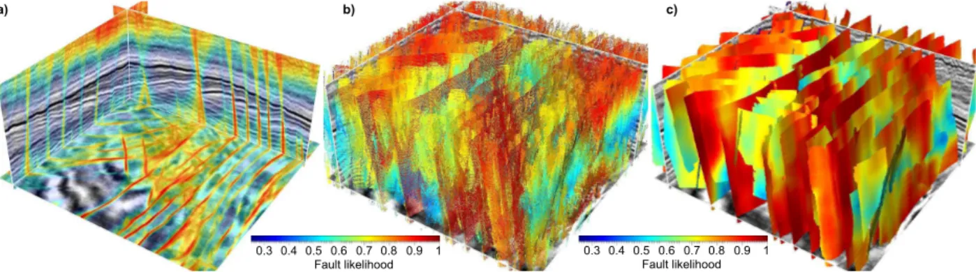
and horizons intersect with the seismic inline and crossline slices in (c). . . 1 Figure 1.2 A 3D seismic image with fault likelihoods (a), fault samples (b), and
fault surfaces. . . 3 Figure 1.3 The fault surfaces in Figure 1.2c is displayed as a fault likelihood image
(a) with mostly null values. This image is used to constrain a
structure-oriented filter so that it smoothes along structures, but not across faults, as shown in (b). Fault slip vectors are then estimated using this smoothed image and the extracted fault surfaces. Only fault throws (c), the vertical components of slips are displayed on the fault
surfaces. . . 3 Figure 1.4 Fault positions (Figure 1.3a) and fault slip vectors (Figure 1.3c) are
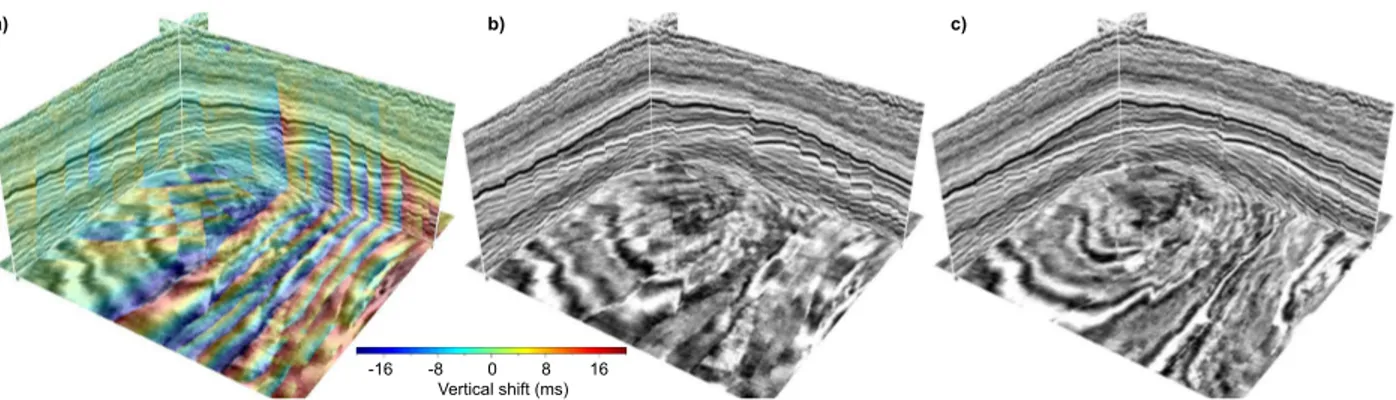
used to compute vertical (a), inline (not shown), and crossline (not shown) unfaulting shifts, which undo the faulting in the original seismic image (b) to compute an unfaulted image(c). . . 4 Figure 1.5 Unconformity likelihood displayed in color (a), and two unconformity
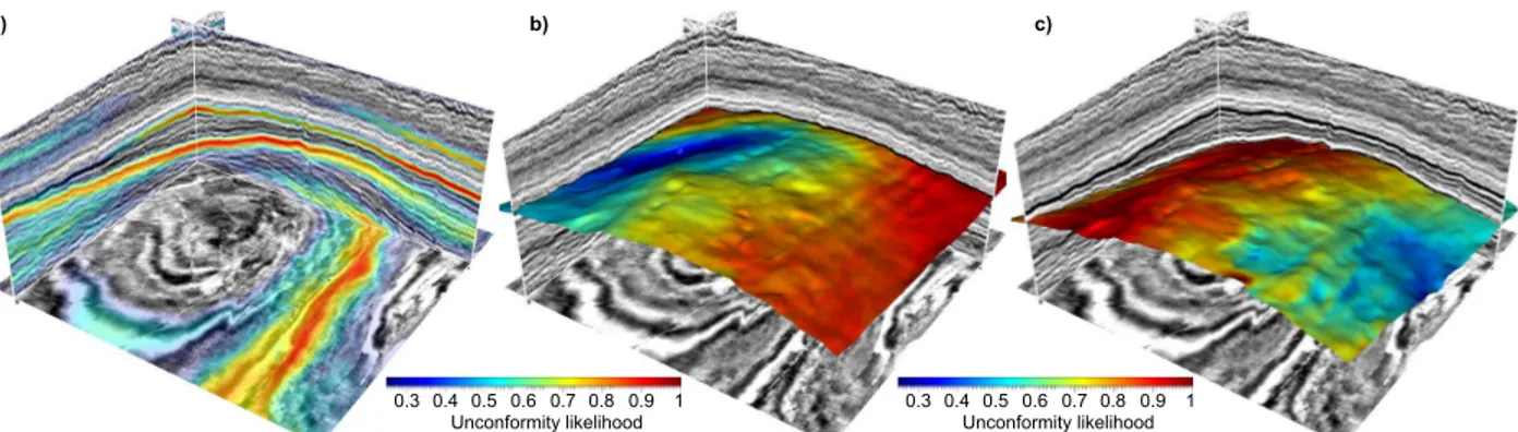
surfaces (b) and (c) extracted on the ridges of the unconformity
likelihoods. . . 6 Figure 1.6 The two unconformity surfaces (Figures 1.5b and 1.5c) extracted from
the unfaulted seismic image, are mapped back to the original seismic
image using the unfaulting shifts, as shown in (a) and (b), respectively. . . 6 Figure 1.7 The unconformities (Figures 1.5b and 1.5c) are used as constraints to
first compute an RGT volume (a) in the unfaulted space, the unfaulted image (b) is then flattened (c) using the RGT volume. . . 8 Figure 1.8 The unfaulting and flattening facilitate extracting any number of
seismic horizons from a seismic image. Shown here are only three
subsets of the extracted horizon surfaces. . . 8 Figure 2.1 A small subset of 3D seismic image displayed with a fault image (a),
Figure 2.2 Fault dip slip (a) is a vector representing displacement, in the dip direction, of the hanging wall side of a fault surface relative to the footwall side. Fault throw is the vertical component of the slip. Fault
strike and dip angles, with corresponding unit vectors are defined in (b). . 12 Figure 2.3 A 3D synthetic seismic image (a) with four faults manually interpreted
in (b). The dashed lines in (b) represent normal faults, while the solid
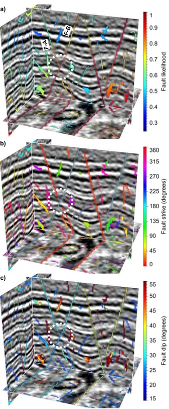
line represents a reverse fault. . . 14 Figure 2.4 A 3D seismic image with fault likelihoods (a), strikes (b) and dips (c)
displayed in color. The dashed white circle in each image indicates one
location where fault F-A intersects fault F-B. . . 16 Figure 2.5 Thinned fault likelihood image (a) has non-zero values only on the
ridges of the fault likelihood image in Figure 2.4a. Fault strikes and dips corresponding to the fault likelihoods are displayed in (b) and (c), respectively. The dashed white circle in each image indicates one
location where fault F-A intersects fault F-B. . . 17 Figure 2.6 The three fault images in Figure 2.5 can be represented by fault
samples displayed as small squares (a). Each square in (a) is colored by fault likelihood and oriented by the strike and dip of the corresponding fault sample. Links are then built among consistent fault samples, and each set of linked fault samples in (b) represents a fault surface that appears opaque in (c), where fault samples are displayed as larger
overlapping squares. . . 19 Figure 2.7 Close-up view (a) of a subset of fault samples from Figure 2.6a. Links
built among nearby fault samples form three sets of linked samples (b) which represent three fault surfaces (or patches). Near the intersection of faults F-A and F-B, fault F-A is separated into two independent patches, and fault F-B has a hole. New fault samples (colored by yellow and blue) are created to merge the fault patches and fill the hole to
construct more complete intersecting fault surfaces (c). . . 20 Figure 2.8 Linked fault samples in Figure 2.6c can be displayed as a fault
likelihood image (with mostly zeros) overlayed with the seismic image in (a). Compared to the thinned fault likelihood image in Figure 2.5a, spurious fault samples have been removed. New fault samples are created at the intersection (dashed white circle) of faults A and B when constructing surfaces. The seismic image in (b) is smoothed along
Figure 2.9 Fault surfaces and fault throws (a) for a 3D seismic image before (b) and after (c) unfaulting. In all image slices, reflectors are more
continuous after unfaulting. . . 28 Figure 2.10 Fault samples colored by fault likelihood (a) are computed, and linked
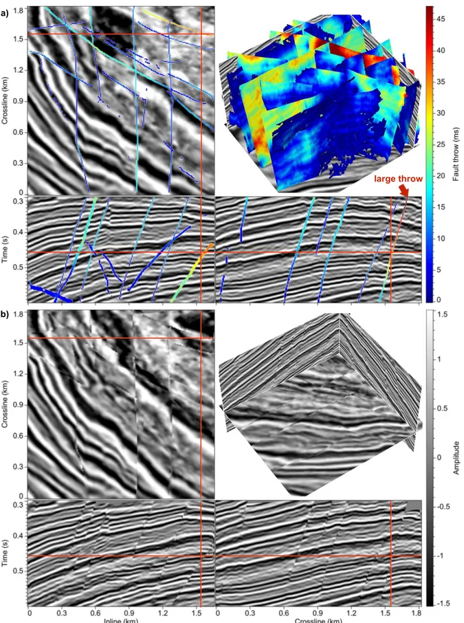
to form fault surfaces (b). . . 30 Figure 2.11 Fault surfaces and fault throws for a 3D seismic image before (a) and
after (b) unfaulting. In all image slices, reflectors are more continuous after unfaulting. The red arrows point to a large-slip fault before and
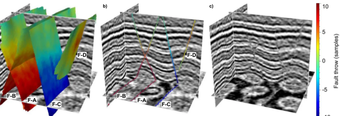
after unfaulting. . . 31 Figure 3.1 A 3D synthetic seismic image with faults colored by fault throws (a), is
significantly distorted when unfaulted (b) by moving only fault blocks while fixing fault positions. Faults (especially fault A) must also be
moved to obtain an unfaulted image (c) with minimal distortions. . . 36 Figure 3.2 Given a 3D seismic image (a), we extract fault surfaces (b) and estimate
fault dip slip vectors for each sample on fault surfaces. Faults in (b) and (c) are colored by fault throws, the vertical components of slip vectors. . 38 Figure 3.3 A fault slip vector t(xa), estimated at each footwall sample adjacent to
a fault, tells us how to correlate the image sample at xa in the footwall
to the corresponding sample xb in the hanging wall. . . 41
Figure 3.4 Vertical (a), inline (b) and crossline (c) components of unfaulting shifts s(x) are computed in the input space using method I. Discontinuities in each component of shifts coincide with fault locations. . . 44 Figure 3.5 Vertical (a), inline (b) and crossline (c) components of unfaulting shifts
s(x) are computed in the input space using method II. Discontinuities
in each component of shifts coincide with fault locations. . . 44 Figure 3.6 Vertical (a), inline (b) and crossline (c) components of unfaulting shifts
in the unfaulted space are converted from those in the input space shown in Figure 3.4. The discontinuities on each component of shifts
are displaced relative to those in Figure 3.4. . . 47 Figure 3.7 Vertical (a), inline (b) and crossline (c) components of unfaulting shifts
in the unfaulted space are converted from those in the input space shown in Figure 3.5. The discontinuities on each component of shifts
Figure 3.8 The input synthetic seismic image (a) is unfaulted (b) using shifts in Figure 3.6 computed by method I, and (c) using shifts in Figure 3.7
computed by method II. . . 48 Figure 3.9 Fault surfaces and slip vectors (a) are first estimated from a 3D seismic
image, and then are used to compute unfaulting vector shifts (b) used below in image unfaulting. Only vertical components of vectors are
shown here. . . 50 Figure 3.10 A 3D seismic image before (a) and after (b) unfaulting. In all image
slices, seismic reflectors are more continuous after unfaulting. For the large-throw fault highlighted by a red arrow in (a), the corresponding fault blocks are significantly moved in (b) to align seismic reflectors on
opposite sides of this fault. . . 51 Figure 3.11 Composite shifts (a) are computed and then used to obtain an
unfaulted and unfolded image (b). . . 52 Figure 3.12 Two horizon surfaces (colored by depth) are extracted using composite
shift vectors that map an image from input space to unfaulted and unfolded space. The vertical component of the composite shift vectors
is displayed in Figure 3.11a. . . 53 Figure 4.1 A 2D synthetic seismic image (a) with an unconformity (red curve) that
is manually interpreted from the termination area to its corresponding parallel unconformity. The estimated seismic normal vectors (red segments in (b)) are smoothed within the termination area, and therefore are incorrect, compared to the true seismic normal vectors
(cyan segments in (b)) that are discontinuous within that area. . . 60 Figure 4.2 Two different seismic normal vector fields estimated using structure
tensors computed with vertically causal (green segments) and
anti-causal (yellow segments) smoothing filters. In (a), the vector fields differ only within the termination area of the unconformity; in (b),
these vector differences are extended to the parallel unconformity. . . 66 Figure 4.3 Unconformity likelihoods, an attribute that evaluates differences
between two estimated seismic normal vector fields (yellow and green segments in Figure 4.2b), before (a) and after (b) thinning highlight
both the termination area and parallel unconformity. . . 68 Figure 4.4 Unconformity likelihoods before (a) and after (b) thinning. . . 68
Figure 4.5 Unconformity likelihoods before (a) and after (b) thinning. Thinned unconformity likelihoods form unconformity surfaces as shown in the
top-right panel in (b). . . 69 Figure 4.6 Vertical (u1) and horizontal (u2) components of the true (a, d) normal
vectors of the synthetic image (Figure 4.1a), the estimated normal vectors (c, f) with the detected unconformity (Figure 4.3b) as
constraints are more accurate than those (b, e) without constraints. . . . 71 Figure 4.7 From the seismic image as shown in Figure 4.4, the vertical (u1) and
horizontal (u2) components of seismic normal vectors estimated using
structure tensors computed with (b, d) and without (a, c) unconformity constraints. . . 72 Figure 4.8 RGT (a) and flattened (c) images generated with inaccurate seismic
normal vectors (Figures 4.7a and 4.7c) and without unconformity constraints. Improved RGT (b) and flattened (d) images with more accurate seismic normal vectors (Figures 4.7b and 4.7d) and
constraints from unconformity likelihoods (Figure 4.4). . . 74 Figure 4.9 Generated RGT volume (a) and flattened (b) 3D seismic image.
Discontinuities in the RGT volume correspond to vertical gaps or
hiatuses (blank areas in (b)) in the flattened image at unconformities. . . 75 Figure 5.1 From a seismic image (a), an RGT volume (b) is computed and then
converted to a horizon volume (c) that maps the seismic image to a
flattened image (d). . . 80 Figure 5.2 Seismic sections (a) and subsections (b) that intersect with a sequence
boundary. The initially horizontal surface (black curve) passes through one control point and is updated iteratively using seismic normal vectors. The dashed green curve denotes the manually interpreted
sequence boundary. . . 87 Figure 5.3 Seismic sections (a) intersect sequence boundaries extracted using one
control point (blue curve) and 19 control points (green curve). (b) and (c) show a 3D view of the extracted surfaces using one control point and 19 control points, respectively. Both of the two surfaces are colored by amplitude. . . 92 Figure 5.4 The same RGT volume (a) as shown in Figure 5.1b, contours (b) of the
RGT volume are horizons in the corresponding seismic image. . . 94 Figure 5.5 A seismic image (a), generated horizon volume (b), and flattened image
Figure 5.6 A seismic image (a) with 3 pairs of interactively interpreted control points (yellow circles, pluses and squares), generated horizon volume
(b) and flattened image (c). . . 102 Figure 5.7 Input seismic image (a) and a corresponding RGT volume (b)
computed with three sets of control points. . . 103 Figure 5.8 The flattened seismic image is sliced at τ = 1.664 (a) and τ = 1.751 (b).
Horizontal slices in a flattened image correspond to seismic horizon surfaces (upper-right panels in (a) and (b), for which color denotes
depth) in an unflattened image. . . 104 Figure 5.9 The RGT volume shown in Figure 5.7b is converted to a complete
horizon volume (a), in which horizontally slicing (h1∼h6) at six different RGT values yields six seismic horizons displayed in (b). The cut-away
ACKNOWLEDGMENTS
People told me that “there are not many Dave Hale in the world”, for me, there is only one Dave. Having a chance to be a student of Dave and work with him, I have to thank another great person Dr. Tom Davis. He kindly encouraged me to also send my PhD application to Dave because he thought my research background was more related to Dave and Dave might be a better advisor for me than him. It has turned out that Tom is correct and Dave is the right advisor to me. I enjoyed every time talking with Dave, his quick thoughts, creative ideas, and valuable suggestions impressed and benefited me much. He taught me how to do research, more importantly, to be an independent thinker and researcher that I am today. He taught me how to write simple, beautiful, and efficient codes. He taught me how to organize a technical paper. He taught me how to efficiently make simple and readable slides. He even taught me how to correctly pronounce a single English word. He bought me a small grammar book “The Elements of Style”, and I carry it everyday in my backpack. What I have learnt from Dave are much more than these above, and the most important thing I got from him is the willing to make anything I already have simpler and better.
I want to thank my minor advisor Dr. Bernard Bialecki. I have been benefited a lot from his mathematic classes to understand and numerically solve the partial different equations that are discussed in this thesis. I appreciate that he was willing to take a lot of time to discuss with me about my research, and these discussions has enriched my thesis. I also want to thank all my teachers, especially the geophysics ones, Dr. Dave Hale, Dr. Paul Sava, Dr. Yaoguo Li, and Dr. Ilya Tsvankin. The geophysical knowledge I learnt from them contributed a lot to my research and thesis.
I want to thank all the faculty of Center for Wave Phenomena (CWP) Dr. Dave Hale, Dr. Paul Sava, Dr. Roel Snieder, and Dr. Ilya Tsvankin for their discussions, assistances, and advices. They all are excellent researchers and scientists. Being working with them is a
wonderful experience for shaping me to be a good researcher as them. I want to thank the CWP students for sharing me with their diverse research ideas, experiences, and cultures. I gained new knowledge and happiness by simply being together with them. I also want to thank the CWP staff Diane Witters, Shingo Sean Ishida, Pamela Kraus, and John Stockwell for their assistance so that I could focus more on my research.
I want to thank all the people I met when I interned in Transform which is now a part of DrillingInfo. They generously shared me with their interests and ideas regarding to seismic interpretation. I want to especially thank Dr. Dean Witte, Stefan Compton, John Neave and Bob Howard. All of them are great programmers and expects on seismic interpretation, and I was inspired and encouraged by them to continue working on my research that are presented in this thesis.
I also want to thank Dr. Sergey Fomel for providing me a great chance to visit the group of Texas Consortium for Computational Seismology (TCCS) and work with people in the Bureau of Economic Geology for six months. It was a pleasant and valuable experience to talk and work with the TCCS students who focused on totally different research topics. Discussions with Dr. Sergey Fomel helped me find possibilities to go beyond my current research presented in this thesis and figure out valuable research projects in the future.
Next but not last, I want to thank my family and friends for their continued support. I want to especially thank my wife Rong for the sacrifice of her study and work in order to better take care of the family. Without her assistance, I do not know how can I finish my PhD program if I need to keep watching our baby girl and keep changing her diapers. Our baby Grace has turned out to be not just a gift or source of happiness for me, she actually keeps training me to be a more efficient worker and sleeper by increasingly decreasing my time for both working and sleeping.
Finally, I want to thank all my thesis committee members Dr. Bernard Bialecki, Dr. Paul Sava, Dr. Tom Davis, Dr. Gongguo Tang, and Dr. Andrzej Szymczak for the constructive discussions with them and their revision of my thesis.
CHAPTER 1 INTRODUCTION
From a 3D seismic image, as shown in Figure 1.1a, one can extract geologic surfaces such as faults (like these vertical surfaces in Figure 1.1b), unconformities (like the two mangenta surfaces in Figure 1.1b and magenta curves in Figure 1.1c), and horizons (like these lateral surfaces in Figure 1.1b and curves in Figure 1.1c). Faults and horizons are important for seismic structural interpretation because they provide structural maps of the subsurfaces. Horizons and unconformities are important for seismic stratigraphic interpretation because they together construct a chronostratigraphic framework. All these geologic surfaces can be useful for seismic lithology interpretation because they can provide geologically reasonable control for extending a lithology interpretation away from wells. Therefore, extracting these surfaces is a critical part of seismic interpretation.
a) b) c)
Figure 1.1: A 3D view of a seismic image (a) and automatically extracted fault (vertical surfaces), unconformity (the two lateral magenta surfaces), and horizon (lateral surfaces) surfaces (b). The unconformities (magenta) and horizons intersect with the seismic inline and crossline slices in (c).
Numerous automatic methods have been proposed to extract all the three types of sur-faces, however, interpreting any of them today typically requires significant manual effort, suggesting that further improvements in automatic methods are feasible and worthwhile.
Moreover, horizons can be especially difficult to extract from a seismic image complicated by both faults and unconformities, as shown in Figure 1.1, because a horizon surface can be dislocated at faults and terminated at unconformities. In this case, we want to first ex-tract fault surfaces, estimate fault slips, and undo the faulting in the seismic image, then to extract unconformities from the unfaulted image with continuous reflectors across faults, finally to use the unconformities as boundary control for image flattening and horizon extrac-tion. In this thesis, I propose 3D seismic image processing methods for (1) fault processing including automatic computation of fault positions, fault slips, and unfaulted images; (2) unconformity processing including automatic extraction of unconformities and estimation of seismic normal vectors at unconformities; (3) image flattening including automatic flattening with constraints from unconformities and semi-automatic flattening with control points or surfaces manually interpreted in the seismic image.
1.1 Fault processing
Automatic interpretation of faults from a seismic image often includes four parts: (1) Fault images or attributes such as semblance (Marfurt et al., 1998), coherency (Marfurt et al., 1999), variance (Randen et al., 2001; Van Bemmel and Pepper, 2000), and fault likelihood (Hale, 2013b) are computed from a seismic image to highlight out fault positions. (2) Then fault surfaces are extracted from these computed fault images using various methods (e.g., Gibson et al., 2005; Hale, 2013b; Pedersen et al., 2002, 2003). (3) From extracted fault surfaces, fault slips are estimated by correlating seismic horizons (Admasu, 2008) or reflectors (Hale, 2013b) on opposite sides of fault surfaces. (4) Computed fault positions and fault slips are finally used to undo the faulting in the seismic image (Luo and Hale, 2013; Wei, 2009; Wei et al., 2005). Although various methods have been proposed for the four parts, the problem of extracting intersecting faults is not well addressed. In addition, extracted fault surfaces are often represented by triangle or quad meshes, which are often more complex than necessary for subsequent processing. Moreover, all the unfaulting methods assume that fault geometries need not change when unfaulting a seismic image. This assumption
makes the unfaulting processing easier, however, often results in unnecessary distortions when unfaulting seismic images with multiple faults and, especially, intersecting faults.
b) a) 0.3 0.4 0.5 0.6 0.7 0.8 0.9 1 Fault likelihood 0.3 0.4 0.5 0.6 0.7 0.8 0.9 1 Fault likelihood c)
Figure 1.2: A 3D seismic image with fault likelihoods (a), fault samples (b), and fault surfaces. b) a) 0.3 0.4 0.5 0.6 0.7 0.8 0.9 1 Fault likelihood c) 0 8 16 24 32 40 Fault throw (ms)
Figure 1.3: The fault surfaces in Figure 1.2c is displayed as a fault likelihood image (a) with mostly null values. This image is used to constrain a structure-oriented filter so that it smoothes along structures, but not across faults, as shown in (b). Fault slip vectors are then estimated using this smoothed image and the extracted fault surfaces. Only fault throws (c), the vertical components of slips are displayed on the fault surfaces.
In Chapter 2, I first describe how to compute images of fault likelihood (Figure 1.2a), strike (not shown), and dip (not shown), and then represent these three images, all at once, by fault samples as shown in Figure 1.2b. Each fault sample corresponds to one and only one seismic image sample, and is displayed as a small square colored by fault likelihood and oriented by strike and dip. I then propose a method to link these oriented fault samples to construct complete fault surfaces without holes, as shown in Figure 1.2c. These surfaces
are really just sets of linked fault samples, they appear as opaque surfaces because fault samples are represented with larger and overlapping squares in Figure 1.2c. These colored fault surfaces can be displayed as a 3D fault likelihood image, with mostly null values, overlaid with the seismic image in Figure 1.3a. This fault image is used to constrain a structure-oriented filter (Fehmers and H¨ocker, 2003; Hale, 2009) so that it smoothes along structures, but not across faults, to obtain the smoothed seismic image shown in Figure 1.3b. This smoothing does what seismic interpreters do visually when estimating fault slips, by bringing seismic amplitudes from within each fault block up to, but not across, the faults. Using this smoothed image and the extracted fault surfaces without holes, I finally estimate fault slips, and display fault throws, the vertical components of the slips, on the fault surfaces shown in Figure 1.3c. c) a) -16 -8 0 8 16 Vertical shift (ms) b)
Figure 1.4: Fault positions (Figure 1.3a) and fault slip vectors (Figure 1.3c) are used to compute vertical (a), inline (not shown), and crossline (not shown) unfaulting shifts, which undo the faulting in the original seismic image (b) to compute an unfaulted image(c).
In Chapter 3, I introduce two methods to compute vertical (Figure 1.4a), inline (not shown), and crossline (not shown) unfaulting shifts for all samples in a seismic image by solving simple equations derived from the precomputed fault positions and fault slip vectors. These computed vector shifts simultaneously move footwalls, hanging walls, and even the faults themselves, to undo faulting in a seismic image, with minimal distortion as shown in Figure 1.4c.
1.2 Unconformity processing
Unconformity extraction from seismic images is important for seismic stratigraphic inter-pretation, because unconformities represent discontinuities in otherwise continuous deposits and hence serve as boundaries when interpreting seismic sequences that represent succes-sively deposited layers. To obtain complete unconformities from a seismic image, we want to extract both angular unconformities with reflector terminations and the corresponding parallel unconformity or correlative conformity with conformable reflectors. Most automatic methods (e.g., Bahorich and Farmer, 1995; Barnes et al., 2000; Hoek et al., 2010; Smythe et al., 2004) can only detect angular unconformities by computing different kinds of attributes that highlight areas of reflector terminations.
In Chapter 4, I propose a method to compute an unconformity likelihood image that highlight both termination areas and the corresponding parallel unconformities as shown in Figure 1.5a. In this method, the unconformity likelihood is defined as the difference between two seismic normal vector fields corresponding to two structure tensor fields constructed from a same seismic image using different smoothing filters. One structure-tensor field is constructed by applying a laterally structure-oriented smoothing filter and a vertical causal filter to each element of the outer products of seismic image gradients. The other one is constructed by applying a same laterally structure-oriented smoothing filter but a vertical anticausal filter. Near the termination area of an unconformity, the reflector structures above and below the unconformity must be different. Therefore, the vertical causal filter, which computes locally averaged structures from above of the unconformity, yields a structure-tensor field that is different from the one constructed with the vertical anticausal filter, which computes locally averaged structures from below. The lateral structure-oriented smoothing filter extends the structure differences, which originate within the termination areas, to the corresponding parallel unconformities and correlative conformities.
Using these lateral and vertical smoothing filters, the two constructed structure-tensors fields and the two corresponding vector fields should be different at both termination area
a) b) c)
0.3 0.4 0.5 0.6 0.7 0.8 0.9 1 Unconformity likelihood 0.3 0.4 0.5 0.6 0.7 0.8 0.9 1
Unconformity likelihood
Figure 1.5: Unconformity likelihood displayed in color (a), and two unconformity surfaces (b) and (c) extracted on the ridges of the unconformity likelihoods.
a) b)
0.3 0.4 0.5 0.6 0.7 0.8 0.9 1 Unconformity likelihood
Figure 1.6: The two unconformity surfaces (Figures 1.5b and 1.5c) extracted from the un-faulted seismic image, are mapped back to the original seismic image using the unfaulting shifts, as shown in (a) and (b), respectively.
and the corresponding parallel unconformity and correlative conformity. Therefore, the un-conformity likelihoods, defined as the differences between the two vector fields, should be relatively high at both the angular unconformities and the corresponding parallel unconfor-mities and correlative conformites as shown in Figure 1.5. From the unconformity likelihood image, two unconformity surfaces (Figures 1.5b and 1.5c) are extracted on the ridges of the unconformity likelihoods.
This method assumes that unconformities are not dislocated by faults, so that the lateral structure-oriented smoothing filter can extend structure differences from termination areas to the corresponding parallel unconformities and correlative conformities. Therefore, if faults
appear in the seismic image, we should perform unfaulting before attempting to detect un-conformities, as in this example shown in Figure 1.5. These unconformity surfaces shown in Figures 1.5b and 1.5c, extracted from the unfaulted image, are then mapped back to the original seismic image, as shown in Figures 1.6a and 1.6b, respectively. These faulted uncon-formities are difficult to extract directly from the original seismic image for any automatic or manual methods.
As applications in Chapter 4, I first use these extracted unconformity surfaces as con-straints for a structure-tensor method (Fehmers and H¨ocker, 2003; Van Vliet and Verbeek, 1995) to more accurately estimate seismic normal vectors at unconformities with multiori-ented seismic reflectors. I then use the more accurate seismic normal vectors, and uncon-formity surfaces as constraints, to compute a flattened image with all flat seismic reflectors within conformable areas and vertical gaps corresponding to the unconformities.
1.3 Image flattening and horizon extraction
Automatic seismic image flattening (Lomask et al., 2006; Parks, 2010; Stark, 2005; Wu and Zhong, 2012a) is a volume process method to identify all horizons in a seismic image by computing a map that transforms the seismic image from the original space into the flattened space. This map can be used to extract any number of horizons from the seismic image. These methods, however, are unable to match horizons across faults unless addi-tional information such as fault slips (Luo and Hale, 2013) and control points across faults (Wu and Hale, 2015b) are provided; also are difficult to deal with horizons terminated at unconformities unless the unconformity surfaces are provided (Wu and Hale, 2015a; Wu and Zhong, 2012a).
For a seismic image complicated only by faults, we could first use the automatic fault processing methods discussed in Chapter 2 and Chapter 3 to estimate fault slips and compute an unfaulted image. Then we could use any flattening method discussed above to compute a flattened or unfolded image from the unfaulted image with continuous reflectors across
b) c) a)
20 40 60 80 100 Relative geologic time
Figure 1.7: The unconformities (Figures 1.5b and 1.5c) are used as constraints to first compute an RGT volume (a) in the unfaulted space, the unfaulted image (b) is then flattened (c) using the RGT volume.
b) c)
a)
Relative geologic time 20 40 60 80 100
Relative geologic time 20 40 60 80 100
Figure 1.8: The unfaulting and flattening facilitate extracting any number of seismic horizons from a seismic image. Shown here are only three subsets of the extracted horizon surfaces.
Figure 1.1a, we still first undo the faulting in the seismic image, as shown in Figure 1.4. Then we extract unconformities from the unfaulted image, as shown in Figure 1.5. Finally we could use the extracted unconformities as constraints, as discussed in Chapter 4, to compute a relative geologic time (RGT) volume shown in Figure 1.7a. This RGT volume, with discontinuous values at unconformties, is applied to the unfaulted image (Figure 1.7b) to compute a flattened image with vertical gaps corresponding the unconformities, as shown in Figure 1.7c.
Horizon extraction is trivial after computing the maps of unfaulting and flattening. For example, I first extract horizontal slices in the unfaulted and flattened space (Figure 1.7c), I then use the RGT volume (Figure 1.7a) to map these horizontal slices back to the unfaulted
space (Figure 1.7b) and obtain curved surfaces, I finally use the unfaulting shifts (Figure 1.4b) to map the curved surfaces back to the original space and eventually obtain curved and faulted surfaces as shown in Figure 1.8. In this way, I can easily compute any number of seismic horizons in the original space. Figure 1.8 shows only three subsets of seismic horizons, which are curved and faulted.
Although all of this image processing can be performed automatically to compute a volume of seismic horizons, limitations inherent in seismic imaging and computing systems suggest that human interaction will continue to be desirable. In Chapter 5, I propose an enhanced semi-automatic method to compute a horizon volume that honors both the seismic image and human interactions. In this method, instead of picking or tracking horizons one at a time as usual, I interactively select scattered sets of points in a 3D seismic image that correspond to multiple horizons, while automatically updating a complete 3D horizon volume to honor those interpreted constraints.
1.4 Publications and proceedings
The work discussed in Chapters 1, 2, 3, 4, and 5 of this thesis have been published in, or submitted to the journals. Below is a full list of my publications:
8. Wu, X., 2016, 3D seismic image processing for subsurface modeling. Computer & Geosciences, to be submitted.
7. Wu, X., 2016, Methods to compute salt likelihoods and extract salt boundaries from 3D seismic images. Geophysics, to be submitted.
6. Wu, X., and G. Caumon, 2016, Simultaneous multiple well-seismic ties with flattened synthetic and real seismograms. Geophysics, to be submitted.
5. Wu, X., and D. Hale, 2016, Automatically interpreting all faults, unconformities, and horizons from 3D seismic images. Interpretation, 4(2), 1-11.
4. Wu, X., and D. Hale, 2016, 3D seismic image processing for faults. Geophysics, 81(2), IM1-IM11.
3. Wu, X., S. Luo, and D. Hale, 2016, Moving faults while unfaulting 3D seismic images. Geophysics, 81(2), IM25-IM33.
2. Wu, X. and D. Hale, 2015, 3D seismic image processing for unconformities: Geo-physics, 80(2), IM35-IM44.
1. Wu, X. and D. Hale, 2015, Horizon volumes with interpreted constraints: Geophysics, 80(2), IM21-IM33.
In addition to the publications above, I have also contributed several conference abstracts: 4. Wu, X., S. Luo and D. Hale, 2015, Moving faults while unfaulting 3D seismic images:
85th Annual Meeting of the Society of Exploration Geophysics, Expanded Abstracts. 3. Wu, X. and D. Hale, 2015, 3D seismic image processing for faults: 85th Annual
Meeting of the Society of Exploration Geophysics, Expanded Abstracts.
2. Wu, X. and D. Hale, 2014, Horizon volumes with interpreted constraints: 84th Annual Meeting of the Society of Exploration Geophysics, Expanded Abstracts.
1. Wu, X. and D. Hale, 2013, Extracting horizons and sequence boundaries from 3D seis-mic images: 83rd Annual Meeting of the Society of Exploration Geophysics, Expanded Abstracts.
CHAPTER 2
3D SEISMIC IMAGE PROCESSING FOR FAULTS
Modified from a paper published on Geophysics Xinming Wu1 and Dave Hale1
2.1 Summary
Numerous methods have been proposed to automatically extract fault surfaces from 3D seismic images, and those surfaces are often represented by meshes of triangles or quadrilat-erals. Such mesh data structures are more complex than the arrays used to represent seismic images, and are more complex than necessary for subsequent processing tasks, such as that of automatically estimating fault slip vectors. To facilitate image processing for faults, we propose a simpler linked data structure in which each sample of a fault corresponds to exactly one image sample. Using this linked data structure, we extracted multiple intersecting fault surfaces from 3D seismic images. We then used the same structure in subsequent processing to estimate fault slip vectors, and to assess the accuracy of estimated slips by unfaulting the seismic images.
2.2 Introduction
Faults like those shown in Figure 3.1 are important geologic surfaces that we can auto-matically extract from 3D seismic images. When extracting a fault surface, we also want to obtain fault strikes, dips, and slip vectors, as illustrated in Figure 2.2.
To extract fault surfaces, fault images (like that shown in Figure 3.1a) are first computed from a seismic image. These fault images indicate where faults might exist. Many methods have been developed to compute fault images using attributes such as semblance (Marfurt et al., 1998), coherency (Marfurt et al., 1999), variance (Randen et al., 2001; Van Bemmel
a) b) c)
Figure 2.1: A small subset of 3D seismic image displayed with a fault image (a), fault samples (b), and fault surfaces (c), all colored by fault likelihood.
footw all hanging wall dip slip heave thro w a) footw all strik e an gle strik e ve ctor d ip v ecto r dip angle b) dip: 0°~90° strike: 0°~360° u v N
Figure 2.2: Fault dip slip (a) is a vector representing displacement, in the dip direction, of the hanging wall side of a fault surface relative to the footwall side. Fault throw is the vertical component of the slip. Fault strike and dip angles, with corresponding unit vectors are defined in (b).
and Pepper, 2000), gradient magnitude (Aqrawi and Boe, 2011) and fault likelihood (Hale, 2013b).
Various methods are also proposed to extract fault surfaces from computed fault images, Pedersen et al. (2002) and Pedersen et al. (2003) propose the ant tracking method to first extract small fault segments, which are then merged to form larger fault surfaces. Similarly, the methods, proposed by Gibson et al. (2005), Admasu et al. (2006) and Kadlec et al. (2008), also try to build larger fault surfaces from smaller patches. Hale (2013b) uses images of fault likelihoods, strikes and dips to construct fault surfaces that coincide with ridges of the fault likelihood image.
From extracted fault surfaces, fault slips can be estimated by correlating seismic reflectors or horizons on opposite sides of the fault surfaces. For example, Borgos et al. (2003) correlate seismic horizons across faults by using a clustering method with multiple seismic attributes. Admasu (2008) propose to use a Bayesian matching of seismic horizons extracted on opposite sides of faults. Aurnhammer and Tonnies (2005) and Liang et al. (2010) use windowed crosscorrelation methods to correlate seismic reflectors across faults. Hale (2013b) uses a dynamic image warping method.
As discussed above, various methods have been proposed to compute fault images, extract fault surfaces and estimate fault slips. However, the problem of extracting intersecting faults, like those shown in Figure 3.1, is not well addressed. For example, the method described by Hale (2013b) assumes that a single seismic image sample can be associated with only one fault, and therefore extracts incomplete fault surfaces, with holes at intersections. Incomplete fault surfaces cause problems for all the above methods used to estimate fault slips, because near holes it is difficult to determine which seismic reflectors should be correlated.
This paper contributes mainly to two aspects of image processing for faults: Firstly, we address the problem of extracting intersecting faults, and obtain complete fault surfaces without holes. Secondly, we propose to represent a fault surface using a linked data structure that is simpler than triangle or quadrilateral meshes often used for fault surfaces.
We first use the method described in (Hale, 2013b) to compute images of fault likelihoods, strikes and dips. Each of the these images has non-null values only at faults, as in the fault likelihood image shown in Figure 3.1a. Therefore, these three fault images can be represented, all at once, by fault samples shown in Figure 3.1b. Each fault sample corresponds to one and only one seismic image sample, and can be displayed as a small square colored by fault likelihood and oriented by strike and dip.
We then use the fault samples in Figure 3.1b to construct fault surfaces, which appear to be continuous, as shown in Figure 3.1c, but are actually only linked lists of the fault samples in Figure 3.1b. In Figure 3.1c, we simply increase the size of squares that are used to
represent fault samples, so that they overlap and appear to form continuous surfaces. Each of these fault surfaces is constructed by linking each fault sample with neighbors above, below, left and right. If any of the four neighbors are missing, we attempt to create them using a method proposed in this paper. In this way, we fill holes and merge separated fault segments to form more complete and intersecting faults as shown in Figure 3.1c.
With more complete surfaces without holes, we are able to more accurately estimate fault slips. To verify the estimated slips, we use them in an unfaulting processing to correlate seismic reflectors across faults.
a) b) a) b) F -A F-B F -C F -D
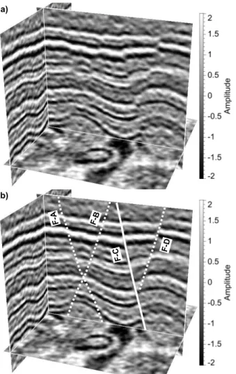
Figure 2.3: A 3D synthetic seismic image (a) with four faults manually interpreted in (b). The dashed lines in (b) represent normal faults, while the solid line represents a reverse fault.
2.3 Fault images
To illustrate our 3D seismic image processing for: (1) computing images of fault likeli-hood, strike and dip, (2) constructing fault samples from thinned fault images, (3) linking fault samples to form fault surfaces, and (4) estimating fault dip slip vectors, we created a synthetic 3D seismic image with normal, reverse, and intersecting faults, as shown in Fig-ure 2.3. This synthetic image contains two intersecting normal faults F-A and F-B, a reverse fault F-C, and a smaller normal fault F-D. While somewhat unrealistic, this synthetic image provides a good test for processing of both normal and reverse faults, and intersecting faults. In 3D seismic images like those shown in Figures 3.1, and 2.3, faults appear as disconti-nuities that are locally planar (or locally linear in 2D slices). This means that, to highlight faults from a seismic image, we do not only look for discontinuities, but rather for discon-tinuities that are locally planar. Fault likelihood, as defined by Hale (2013b), is one such measure of locally planar discontinuity. Therefore, we use Hale’s (2013b) method to compute fault likelihood (Figure 2.4a), while at the same time estimating fault strike (Figure 2.4b) and dip (Figure 2.4c). The fault likelihood image indicates where faults might exist, while the strike and dip images indicate their orientations.
In computing these fault images, this method scans over a range of possible combinations of strike and dip to find the one orientation that maximizes the fault likelihood, for each image sample (Hale, 2013b). The maximum fault likelihood for each image sample is recorded in the fault likelihood image (Figure 2.4a), and the strike and dip angles that yield the maximum likelihood are recorded in the fault strike (Figure 2.4b) and dip (Figure 2.4c) images, respectively. In the fault likelihood image in Figure 2.4a, we expect relatively high values in areas where faults might exist. In the fault strike (Figure 2.4b) and dip (Figure 2.4c) images, we expect strike and dip angles to be accurate only where faults are likely, that is, where fault likelihoods are high.
As discussed by Hale (2013b), a significant limitation of this scanning method is in dealing with intersecting faults. Because only a single fault likelihood value, and its corresponding
c) a) b) F -A F-B
Figure 2.4: A 3D seismic image with fault likelihoods (a), strikes (b) and dips (c) displayed in color. The dashed white circle in each image indicates one location where fault F-A intersects fault F-B.
a) b) c) F -A F-B
Figure 2.5: Thinned fault likelihood image (a) has non-zero values only on the ridges of the fault likelihood image in Figure 2.4a. Fault strikes and dips corresponding to the fault likelihoods are displayed in (b) and (c), respectively. The dashed white circle in each image indicates one location where fault F-A intersects fault F-B.
fault strike and dip are recorded for each image sample, this method implicitly assumes that each image sample can be associated with only one fault. This assumption is not valid for samples where two or more faults intersect. For example, in the intersection area highlighted in Figure 2.4, fault likelihoods, strikes and dips for only fault F-B have been recorded, and the information corresponding to fault F-A is missing there. Fault likelihoods of fault F-A might also be high near this intersection, but have been discarded together with corresponding strikes and dips, only because they were smaller than the fault likelihoods computed for fault F-B. Therefore, fault surfaces directly extracted from such fault images often have holes, especially near fault intersections. We describe below a method to fill holes when constructing fault surfaces.
We do not expect faults to be as thick as the features apparent in the fault likelihood image in Figure 2.4a. Therefore, we keep only the values on the ridges of fault likelihood, and set values elsewhere to be zero, to obtain a thinned fault likelihood image shown in Figure 2.5a. We also keep strike and dip angles for only the samples with non-zero values in Figure 2.5a, to obtain the corresponding thinned fault strike (Figure 2.5b) and dip (Fig-ure 2.5c) images. These thinned fault images have non-null values only for samples that might be on faults.
We again observe that fault likelihoods, strikes and dips of fault F-A are missing in the intersection area (dashed white circles in Figure 2.5) because of the limitation discussed above. We also observe that some non-null values appear where faults do not exist. The reason for this is that, in the scanning process, we assume only that faults are locally planar discontinuities. We will discuss below additional conditions that must be satisfied for the non-null samples in Figure 2.5 to be considered as faults.
2.4 Fault samples and surfaces
Notice that most samples in thinned fault images shown in Figure 2.5 are null. For this reason, we use fault samples to more efficiently represent the three fault images with less computer memory. We then extract fault surfaces from the fault samples, and represent the
surfaces using simple and convenient data structures. 2.4.1 Fault samples
Because most samples in the images of fault likelihood (Figure 2.5a), strike (Figure 2.5b) and dip (Figure 2.5c) are null, we can display the three images, all at once, as fault samples shown in Figure 2.6a, and more clearly in Figure 2.7a. Each fault sample is displayed as a colored square. The color of each square denotes fault likelihood, while the orientation of each square represents fault strike and dip. Fault samples exist only at positions where thinned fault likelihoods are non-null, and each fault sample corresponds to one and only one image sample. Therefore, these fault samples contain exactly the same information represented in the thinned fault images shown in Figure 2.5.
Most fault samples, especially those with high fault likelihoods, are aligned approximate planes, consistent with locally planar fault surfaces. Some misaligned fault samples, often with low fault likelihoods, are also observed in Figures 2.6 and 2.7. These misaligned samples, however, cannot be linked together to form locally planar fault surfaces of significant size.
a) b) c) F-A F-B F-C F-D F-A F-B F-C F-D
Figure 2.6: The three fault images in Figure 2.5 can be represented by fault samples displayed as small squares (a). Each square in (a) is colored by fault likelihood and oriented by the strike and dip of the corresponding fault sample. Links are then built among consistent fault samples, and each set of linked fault samples in (b) represents a fault surface that appears opaque in (c), where fault samples are displayed as larger overlapping squares.
b) c) a) F-A F-B F -A F-B F -A
Figure 2.7: Close-up view (a) of a subset of fault samples from Figure 2.6a. Links built among nearby fault samples form three sets of linked samples (b) which represent three fault surfaces (or patches). Near the intersection of faults F-A and F-B, fault F-A is separated into two independent patches, and fault F-B has a hole. New fault samples (colored by yellow and blue) are created to merge the fault patches and fill the hole to construct more complete intersecting fault surfaces (c).
2.4.2 Fault surfaces
Fault surfaces are often represented by meshes of triangles or quadrilaterals (Hale, 2013b). However, these mesh structures are unnecessary for the image processing described in this paper.
For example, to estimate fault slips, we must analyze seismic image samples alongside faults. This means that we must know how to walk vertically up and down (tangent to fault dip), and horizontally left and right (tangent to fault strike), on a fault surface, and thereby to access seismic image samples adjacent to the fault. The quadrilateral mesh discussed by Hale (2013b) is one way to efficiently access seismic image samples alongside a fault. In this paper, we use a simpler linked data structure, shown in Figures 2.6b, 2.7b and 2.7c, to find seismic image samples adjacent to faults.
2.4.3 Linking fault sample neighbors
To link fault samples into fault surfaces, we use their fault likelihoods, strikes and dips. We grow a fault surface by linking nearby fault samples with similar fault attributes,
begin-ning with a seed sample that has sufficiently high fault likelihood. Remember that each fault sample corresponds to exactly one sample of the seismic image. This means that we can use the image sampling grid to efficiently search for neighbor samples that should be linked. In a 3D sampling grid, each fault sample has 26 adjacent grid points in a 3 × 3 × 3 cube centered at that sample, but most of these adjacent grid points will not have a fault sample. At these adjacent grid points, we search for up to four neighbor fault samples, above and below (in directions best aligned with fault dip), left and right (in directions best aligned with fault strike).
To find a neighbor above, we need only consider the upper 9 adjacent points in the 3 × 3 × 3 cube of grid points. Among these 9 grid points, we search for a fault sample that lies nearest to the line defined by the center fault sample and its dip vector. Similarly, we search for a neighbor below among the lower 9 adjacent grid points.
To find a neighbor right and left, we need only search in the 8 adjacent grid points with the same depth as the center fault sample in the 3 × 3 × 3 cube. The right neighbor is the one located in the strike direction and nearest to the line defined by the center fault sample and its strike vector. The left neighbor is the one in the opposite direction and closest to the same line.
The fault samples (up to four) obtained in this way are only candidate neighbors. To be considered as valid neighbors and then linked to the center sample, they must have fault likelihoods, dips and strikes similar to those for the center sample.
The processing above is repeated for each fault sample neighbor until no more neighbors can be found, to obtain a linked list of fault samples (Figure 2.7b). Then a new seed with sufficiently high fault likelihood is chosen from unlinked samples for growing a new fault surface. This process ends when no remaining unlinked fault samples have sufficiently high fault likelihood.
Some samples linked in this way may not correspond to faults. We discard surfaces with small numbers of linked samples, and keep only those with significant sizes. For an
example, in Figure 2.7b, we have kept only the three largest surfaces constructed from the fault samples in Figure 2.7a. Other fault samples (such as these colored by green and blue in Figure 2.7a) are then ignored in subsequent processing.
As shown in Figure 2.7b, each sample in a fault surface is linked to up to four neighbors. Some neighbors might be missing, and this is in fact necessary, because faults are not per-fectly aligned with the sampling grid of a 3D seismic image, and also because faults are not strictly planar surfaces.
However, some neighbors may be missing because the seismic image is noisy. And where faults intersect, fault samples constructed directly from fault images may be missing, as shown in Figure 2.7a. These missing fault samples can cause holes within a fault surface, like the fault F-B shown in Figure 2.7b, and can yield gaps which separate a fault surface into independent patches, like those of fault F-A shown in Figure 2.7b. To fill in these holes and gaps to construct more complete fault surfaces, we must interpolate missing fault samples, as shown in Figure 2.7c.
2.4.4 Interpolating missing neighbors
During the processing discussed above for linking neighbors to a fault sample, if any of the neighbors above, below, left or right are missing, we try to create them. We do not first construct fault surfaces or patches with holes (missing neighbors) as shown in Figure 2.7b, and then fill holes in each of the constructed fault surfaces or patches, because in this way we cannot merge fault patches to form more complete fault surface. Instead, we check for missing neighbors, and create them as we grow fault surfaces, and thereby directly obtain complete fault surfaces without holes as shown in Figure 2.7c.
Remember that each fault sample contains three attributes: fault likelihood, strike and dip. This means that, if we want to create a missing fault sample, we must know not only its position, but also its corresponding fault attributes. Therefore, instead of directly creating fault samples, we first construct three fault images and then create fault samples from these images. Recall that we find neighbors for a fault sample from only the adjacent grid points
in a 3 × 3 × 3 cube that is centered at that fault sample. This means that, to create a missing neighbor, we need only create adjacent fault samples, and then determine whether any of them could be the missing neighbor.
To create fault samples within a 3 × 3 × 3 cube, we must create fault images in a slightly larger cube, because fault samples are located on the ridges in a fault likelihood image, and additional image samples are needed to find these ridges. Therefore, we construct the new small images of fault likelihood, strike and dip in a 5 × 5 × 5 cube.
To construct a fault likelihood image in a 5 × 5 × 5 cube centered at the fault sample with missing neighbors, we first search nearby to find fault samples that have fault attributes similar to those for the center sample. For all examples in this paper, we search for these nearby samples in a 31 × 31 × 31 cube. Suppose that we find N existing fault samples, we then construct a 5 × 5 × 5 fault likelihood image by accumulating weighted anisotropic Gaussian functions generated from the N existing fault samples found nearby:
f (xi) = N
X
k=1
f (xk)g(xk− xi), (2.1)
where f (xi) denotes a fault likelihood value computed for the i-th grid point in the 5 × 5 × 5
cube, and xi denotes the position of that grid point. Here, f (xk) denotes the known fault
likelihood of the k-th nearby fault sample, and g(x) is an anisotropic Gaussian function computed for this k-th fault sample:
g(x) = exp(−1 2x
⊤R⊤SRx). (2.2)
Here, R and S are 3 × 3 matrices:
R= u⊤k v⊤k w⊤k , and, S = 1 σ2 u 0 0 0 σ12 v 0 0 0 1 σ2 w , (2.3)
where the unit column vectors uk and vk are the dip and strike vectors of the k-th nearby
fault sample, respectively. The vector wk= uk× vk is normal to the plane of the k-th fault
strike (v) and normal (w) directions, respectively. The matrix R rotates the anisotropic Gaussian to be aligned with the vectors uk, vk and wk. Because a fault should be locally
planar in strike and dip directions, we set the half-widths σu and σv to be larger than σw, so
that the Gaussian to be accumulated extends primarily in the fault strike and dip directions. For all examples in this paper, we set σw = 1 and σu = σv = 15 samples.
To create fault samples located on ridges of a fault likelihood image, we must also con-struct images of fault strikes and dips. Therefore, when accumulating anisotropic Gaussian functions for the i-th sample in the 5 × 5 × 5 cube, we also accumulate weighted outer products of normal vectors for that sample:
D(xi) =
N
X
k=1
f (xk)g(xk− xi)wkw⊤k. (2.4)
We then apply eigen-decomposition to the 3 × 3 matrix D(xi), and choose the eigenvector corresponding to the largest eigenvalue to be the normal vector wi for the i-th sample in the
5 × 5 × 5 cube. From each normal vector wi, we then compute strike and dip angles for this
i-th sample.
After construct the three 5 × 5 × 5 fault images, we then create fault samples on the ridges of the fault likelihood image, and search for missing neighbors among these new fault samples. Again, the conditions discussed in the previous section must be satisfied when finding neighbors from these new samples. If no valid neighbors can be found, we stop linking neighbors to the center fault sample.
Figure 2.7c shows new fault samples created in this way, and colored by yellow and blue, for two different fault surfaces. Using both newly created and original fault samples, we are able to construct intersecting fault surfaces without holes, as shown in Figure 2.7c.
Figure 2.6b shows the four fault surfaces extracted from the 3D seismic image by using the method discussed above. They can be displayed as opaque fault surfaces, as in Figure 2.6c, by simply increasing the size of each square so that they overlap and appear to form continuous surfaces.
b) b) a) F -A F-B
Figure 2.8: Linked fault samples in Figure 2.6c can be displayed as a fault likelihood image (with mostly zeros) overlayed with the seismic image in (a). Compared to the thinned fault likelihood image in Figure 2.5a, spurious fault samples have been removed. New fault samples are created at the intersection (dashed white circle) of faults A and B when constructing surfaces. The seismic image in (b) is smoothed along structures, but not across the faults.
However, these surfaces are really just linked fault samples. As shown in Figure 2.7c, the samples on a surface are linked above and below in the fault dip direction, left and right in the strike direction, and no holes are apparent. These links enable us to iterate among seismic image samples adjacent to a fault, in both dip and strike directions, as we estimate fault slips.
Recall that each sample in a fault surface corresponds to exactly one sample of the seismic image, therefore, fault likelihoods for the surfaces shown in Figure 2.6c can be easily
displayed as a 3D fault likelihood image (with non-null values only at faults) overlayed with the seismic image in Figure 2.8a. Compared to the thinned fault likelihood image in Figure 2.5a, spurious fault samples have been removed and new fault samples have been created near the intersection (dashed white circle) of faults A and B.
We create this fault likelihood image to constrain a sturcture-oriented filter (Fehmers and H¨ocker, 2003; Hale, 2009) so that it smoothes along structures, but not across faults, to obtain the smoothed seismic image shown in Figure 2.8b. We use this smoothed image in the next section for estimating fault slips, because the smoothing does what seismic interpreters do visually when estimating fault slips, by bringing seismic amplitudes from within each fault block up to, but not across, the faults.
2.5 Fault dip slips
In a 3D seismic image, fault strike slips are typically less apparent than dip slips. There-fore, we have not attempted to estimate fault slips in the strike direction. As shown in Figure 2.2a, fault dip slip is a vector representing displacement, in the dip direction, of the hanging wall side of a fault surface relative to the footwall side. Fault throw is the vertical component of slip. If we know the fault throw and the fault surface with linked samples, as in Figure 2.7c, then we can walk up or down the fault in the dip direction to compute the two corresponding horizontal components of dip slip. Therefore, to estimate dip slips, we first estimate fault throws.
2.5.1 Fault throws
To estimate fault throws, we compute vertical components of shifts that correlate seismic reflectors on the footwall and hanging wall sides of a fault surface. As discussed by Hale (2013b), this correlation can be difficult. The drawing of a fault in Figure 2.2a is a very simple case, where the fault surface is entirely planar, and fault throw is constant for the entire surface. In reality, fault throws may vary significantly within a fault surface, and this variation can make windowed crosscorrelation methods (Aurnhammer and Tonnies, 2005;
Liang et al., 2010) fail when fault throws vary within a chosen window size.
To avoid choosing windows in which throws are assumed to be constant, we use the dynamic image warping method (Hale, 2013a,b) to estimate fault throws. Compared to windowed crosscorrelation methods, dynamic image warping is more accurate, especially when the relative shifts between two images vary rapidly. Moreover, this method enables us to impose constraints on the smoothness of estimated shifts. These constraints are important in fault throw estimation, because we expect throws to vary smoothly and continuously along a fault, even where they may increase or decrease rapidly.
The dynamic image warping method described in Hale (2013a) cannot be used directly to estimate fault throws. This method assumes images to be warped (aligned) are regularly sampled. In practice, a fault is generally not planar; instead, it is often curved and sometimes cannot be projected onto a plane (e.g., Walsh et al., 1999). Therefore, images extracted from opposite sides of a fault are not regularly sampled 2D images as required for dynamic image warping. The dynamic warping method must be modified for fault throw estimation.
Hale (2013b) represents a fault surface as a quad mesh that facilitates computation of differences between seismic amplitudes on opposite sides of a fault. Those amplitude differences are computed for every sample on the fault, for a range of shifts that correspond to different fault throws. The fault throws computed by dynamic warping are shifts that minimize these seismic amplitude differences, subject to constraints that those shifts must vary smoothly along the fault surface.
In this paper, we use the same dynamic warping process, but with seismic amplitude differences computed using the simpler linked data structure illustrated in Figure 2.7c. It is advantageous that the fault surfaces represented in Figure 2.7c do not have holes. Holes in fault surfaces like those shown in Figure 2.7b make it difficult to determine which samples of the seismic image should be used when computing the amplitude differences required for dynamic warping. Holes also make it difficult for the dynamic warping method to enforce the constraints that fault throws vary smoothly. For these reasons, fault throws estimated
using fault surfaces like those shown in Figure 2.7c are more accurate than those for fault surfaces with holes, like those shown in Figure 2.7b.
a) b) c) F-A F-B F-C F-D F-A F-B F-C F-D
Figure 2.9: Fault surfaces and fault throws (a) for a 3D seismic image before (b) and after (c) unfaulting. In all image slices, reflectors are more continuous after unfaulting.
Fault surfaces in Figure 2.9a are the same surfaces shown in Figure 2.6c, but colored by fault throws estimated using the method discussed above. We observe that fault throws estimated for each surface vary smoothly, as expected. Also, fault throws for fault F-C are negative because this fault is a reverse fault. Estimated fault throws for faults F-A, F-B, and F-C generally increase in magnitude with depth, while throws for the smaller fault F-D first increase, then decrease with depth. An unfaulting processing described below verifies the accuracy of these estimated fault throws.
With fault throw estimated for each fault sample in a fault surface, we can use the links and the dip vectors u to walk upward or downward, to determine fault heave for that sample. Fault heave is the horizontal component of a slip vector, and is decomposed into horizontal inline and crossline components. In this way, a slip vector for each fault sample is computed and represented by a vertical component in the traveltime or depth direction, and two horizontal components in inline and crossline directions. The two horizontal components are computed but not shown in this paper.
If the computed fault dip slip vectors are accurate, then we should be able to undo faulting apparent in the seismic image, that is, to correctly align seismic reflectors on opposite sides
of faults.
2.5.2 Unfaulted images
Hale (2013b) uses seismic image unfaulting (Luo and Hale, 2013) to verify the accuracy of estimated dip slips. In their unfaulting method, the dip slips are assumed to be displacements of image samples adjacent to hanging wall sides of faults, and slips for image samples adjacent to footwall sides of faults are assumed to be zero. Because each sample on a fault always lies between two samples of a seismic image, it is easy to locate and set the slips for each pair of footwall and hanging wall samples. Luo and Hale (2013) then simply interpolate all three components of slip vectors for all samples of the seismic image between faults, so that slips away from faults are smoothly varying. Unfortunately, where faults intersect, the assumption that slips on the footwall sides of faults are zero yields unnecessary distortions in the unfaulted seismic image.
Here we use a different method described by Wu et al. (2016) to unfault a seismic image, and thereby verify our estimated dip slips. In this method, vector shifts are computed for all samples in the seismic image by solving partial differential equations derived from the fault slip vectors estimated at faults. This method moves both footwalls and hanging walls, and even faults themselves, simultaneously, to undo faulting with minimal distortion.
Figure 2.9b shows the seismic image with faults colored by estimated fault throws, the vertical components of estimated dip slip vectors. These fault throws, as well as the two horizontal components of the slips, are used in Wu et al. (2016) to obtain the unfaulted image shown in Figure 2.9c. In the unfaulted image, seismic reflectors are well aligned across faults, including the intersecting normal faults and the reverse fault. This unfaulted image illustrates that estimated fault slip vectors are accurate to within the resolution of the seismic image.
a)
b)
Figure 2.10: Fault samples colored by fault likelihood (a) are computed, and linked to form fault surfaces (b).
a)
large throw
b)