THESIS
AIR CONCENTRATION AND BULKED FLOW ALONG A CURVED, CONVERGING STEPPED CHUTE
Submitted by Blake W. Biethman
Department of Civil and Environmental Engineering
In partial fulfillment of the requirements For the Degree of Master of Science
Colorado State University Fort Collins, Colorado
Spring 2020
Master’s Committee:
Advisor: Robert Ettema
Co-Advisor: Christopher Thornton Ellen Wohl
Copyright by Blake William Biethman 2020 All Rights Reserved
ABSTRACT
AIR CONCENTRATION AND BULKED FLOW ALONG A CURVED, CONVERGING STEPPED CHUTE
This thesis focuses on the air-entrainment performance of a stepped spillway of unique form. The performance was determined using a hydraulic model constructed at a length scale (prototype length/model length) of 24. The new stepped spillway is part of the Gross Reservoir Expansion (GRE) project, which by 2025 is expected to raise the existing Gross Dam about a third of its current height. The stepped spillway will be the tallest stepped spillway in the United States. The model spillway consisted of a chute whose step dimensions, vertical to horizontal, were 0.051 m by 0.025 m, resulting in a chute slope (V:H) of 2.0 and a chute angle of 63.4o. Additionally, the chute conformed, in planform, to the curved planform of raised Gross Dam. At the spillway’s crest, that radius of curvature, at model scale, was 22.2 m. The chute width converged by about 20% from the top of the chute to the stilling basin at the base of the chute. The chute’s steepness, height, curvature and convergence made the chute’s geometry unique among existing stepped spillways.
The evaluation involved measurements of air entrainment and flow velocity along the stepped chute, for which the skimming flow regime prevailed for discharge larger than about 9% of the spillway’s design discharge. To date, the effect on water flow and air entrainment of chute curvature in stepped spillways had not been investigated. The investigation was facilitated from measurements obtained using a dual-tip conductivity probe, which detected the instantaneous
void fraction of the air-water mixture. The probe also enabled measurement of the velocity of the bulked flow along the chute.
The study showed that, when the chute conveyed the design discharge (at model scale, 0.347 m3/s), streamwise values of air concentration and flow depth (bulked with entrained air) were basically constant near the bottom of the chute. Additionally, the chute’s planform curvature resulted in non-uniform flow across the chute. At the design discharge, and near the bottom of the chute, the flow depth along the chute’s centerline was nominally about 30% greater than the flow depth at the sidewall. When the chute’s curvature was accounted for, the water surface along the centerline of the chute was approximately level with the water surface near the sidewall. Further, the depth-averaged concentration of entrained air near the bottom of the chute decreased with increasing water discharge. The chute’s converging sidewalls mildly affected the flow near the sidewalls, causing slight increases in flow depth and reductions in flow velocity. These changes, though noticeable, were negligible in terms of spillway performance because of their magnitude.
ACKNOWLEDGEMENTS
The research conducted as part of this thesis would not have been possible without the support and mentorship of my advisor and co-advisor, Drs. Robert Ettema and Christopher Thornton, to whom I am most grateful for giving me the opportunity to participate in the hydraulic model study of the Gross Dam spillway. Additional thanks are given to the laboratory staff at the ERC for their expertise and assistance. I am thankful for the funding provided by Denver Water, and to those individuals with whom I worked during the completion of this work: Dr. Ed Kempema, Ali Reza Nowrooz Pour, Alireza Fakhri, Selina Tasdelen, Taylor Hogan and all other graduate- and undergraduate-staff at the ERC. Thanks, also, to Dr. Ellen Wohl for serving on my
committee. Finally, a special thanks to my friends and family for their love and support during my graduate studies.
TABLE OF CONTENTS ABSTRACT ... ii ACKNOWLEDGEMENTS ... iv LIST OF TABLES ... ix LIST OF FIGURES ... xi LIST OF SYMBOLS ... xv 1 INTRODUCTION ... 1 1.1 Motivation ... 1 1.2 Objectives of Thesis ... 1 1.3 Background ... 2
1.4 Gross Reservoir Expansion ... 3
1.5 Format of Thesis... 4
2 LITERATURE REVIEW ... 5
2.1 Introduction ... 5
2.2 Air Entrainment and Concentration ... 6
2.3 Friction Factor ... 8
2.4 Equilibrium Flow Conditions ... 10
2.5 Vertical Distribution of Air Concentration ... 13
2.6 Longitudinal Development of Air Concentration ... 14
2.7 Bulk-Flow Velocity ... 18
2.8 Sidewall Height ... 19
2.9 Similarity ... 20
2.9.1 Scale Effects... 21
3.1 Introduction ... 23
3.1.1 Model Dimensions and Layout ... 23
3.2 Similitude and Model Scaling ... 27
3.3 Measurements... 27 3.3.1 Air Concentration... 28 3.3.2 Bulk-Flow Velocity ... 30 3.4 Instrumentation... 31 3.4.1 Conductivity Probe ... 31 3.4.2 Discharge ... 33
4 RESULTS & ANALYSES ... 35
4.1 Introduction ... 35
4.2 General Flow Conditions ... 39
4.2.1 Equilibrium Flow Conditions ... 41
4.3 Air Concentration ... 42
4.3.1 Equilibrium Flow Conditions ... 42
4.3.2 Measurements Along the Chute Sidewall ... 44
4.3.3 Variation with Water Discharge ... 49
4.3.4 Measurements Across the Chute ... 56
4.3.5 Repeatability of Water-Surface Measurements ... 63
4.3.6 Time-Series Record of Air-Concentration Data ... 65
4.4 Bulk-Flow Velocity ... 73
4.4.1 Measurements Along the Chute Sidewall ... 73
4.4.2 Variation with Water Discharge ... 75
4.4.3 Measurements Across the Chute ... 80
4.6 Comparison of Results with Existing Relationships ... 88
4.6.1 Vertical Distributions of Air Concentration (in Equilibrium Flow) ... 88
4.6.2 Equilibrium Flow Conditions ... 89
4.6.3 Velocity Exponent ... 92
4.6.4 Friction Factor ... 95
4.6.5 Time-Series ... 96
4.6.6 Pier Effect ... 96
5 CONCLUSIONS & RECOMMENDATIONS ... 98
5.1 Main Conclusions ... 98
5.2 Recommendations for Further Research ... 100
6 REFERENCES ... 102
Appendix A FLOW CONDITION PHOTOS ... 106
A.1 0.014 m3/s < Q < 0.028 m3/s ... 106 A.2 Q = 0.028 m3/s ... 109 A.3 Q = 0.085 m3/s ... 116 A.4 Q = 0.133 m3/s ... 118 A.5 Q = 0.142 m3/s ... 120 A.6 Q = 0.170 m3/s ... 122 A.7 Q = 0.198 m3/s ... 124 A.8 Q = 0.227 m3/s ... 126 A.9 Q = 0.255 m3/s ... 128 A.10 Q = 0.283 m3/s ... 130 A.11 Q = 0.311 m3/s ... 132
A.12 Q = 0.347 m3/s (the design discharge) ... 134
B.1 Skimming Flow ... 140
B.2 Nappe Flow... 144
B.3 Transition Flow... 145
Appendix C OPERATION OF THE CONDUCTIVITY PROBE ... 146
C.1 Overview ... 146
C.2 Probe Setup ... 147
C.3 Data Collection ... 153
C.4 Data Conversion ... 154
C.5 Data Processing ... 157
LIST OF TABLES
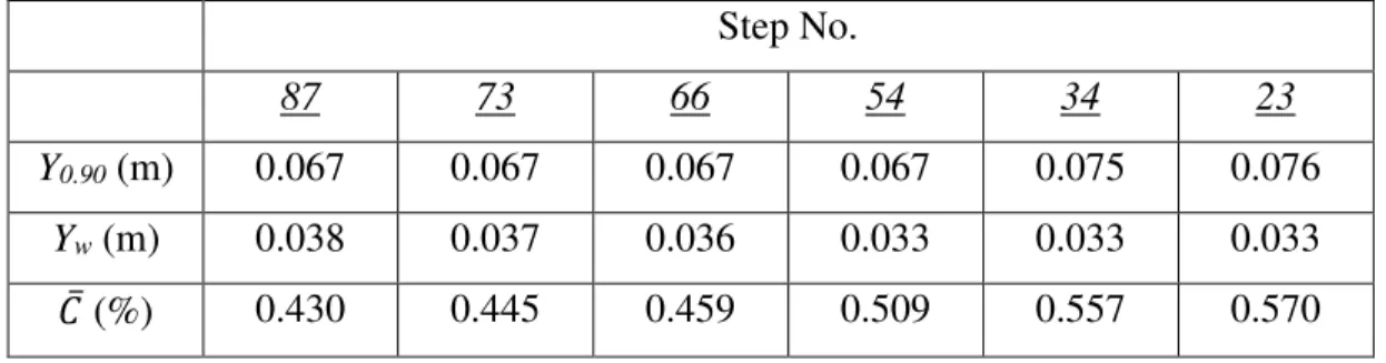
Table 2.1. Coefficients for Wood’s distribution (Chanson, 1993). ... 13 Table 3.1. Model dimensions ... 24 Table 3.2. Values of variables at model scale ... 27 Table 4.1. Values of Y0.90, 𝐶and Yw measured at the chute-sidewall and centerline positions when
the chute conveyed the design discharge ... 43 Table 4.2. The longitudinal variations of Y0.90, Yw and 𝐶 measured near the chute’s right sidewall
when the chute conveyed the design discharge. ... 48 Table 4.3. The variations with water discharge of Y0.90, 𝐶 and Yw at the chute-sidewall position of
step 23. ... 50 Table 4.4. The variations with water discharge of Y0.90, 𝐶 and Yw at the chute-centerline position
of step 23. ... 53 Table 4.5. The distributions across the chute of Y0.90, 𝐶 and Yw when the chute conveyed the
design discharge. ... 60 Table 4.6. Repeated measurements of the value Y0.90along the chute’s centerline position of step
23 when the chute conveyed its design discharge. Run IDs 01-02 are the measurements that produced the original value of Y0.90 (0.096 m), and IDs 1-10 are the repeated measurements that
produced the new value (Y0.90 = 0.095 m). ... 64
Table 4.7. Repeated measurements of the value Y0.90 at chute position b/B = 0.21 of step 23 when
the chute conveyed its design discharge. Run IDs 01-02 are the measurements that produced the original value of Y0.90 (0.074 m), and IDs 1-5 are the repeated measurements at the flow depth Y
= 0.075 m. ... 65 Table 4.8. Variance in C when data were averaged over sub-intervals of 1.0, 5.0 and 10.0 sec. . 67 Table 4.9. Longitudinal variations of Y0.90, V0.90 and N, measured near the right sidewall when
the chute conveyed its design discharge. ... 75 Table 4.10. Variations with water discharge of Y0.90, V0.90 and N at the chute-sidewall position of
step 23. ... 78 Table 4.11. Variations with water discharge of Y0.90, V0.90 and N at the chute-centerline position
Table 4.12. Values of V0.90, 𝑉 and N across the chute, measured along step 23 when the chute
LIST OF FIGURES
Figure 1.1. A panoramic view of Gross Reservoir and Dam. ... 2
Figure 1.2: A comparison of the existing Gross Dam and proposed Gross Dam. On left, the existing structure with crest elevation of 2221.9 m, and on right, the proposed structure with crest elevation of 2261.9 m. [https://grossreservoir.org/construction/raising-a-dam/] ... 3
Figure 2.1: A plot of stepped chute flow regimes, with experimental data sources given in the legend (Frizell & Frizell, 2015). Along the ordinate, dc refers to the critical flow depth, herein referred to as Yc. ... 6
Figure 2.2. Reduction in f with increase in Yc/h for 𝜃=53.1o (Matos & Meireles, 2014). ... 9
Figure 2.3. Conjectured regions of non-equilibrium flow (Wood, 1983, based on data from Straub & Anderson, 1958). ... 11
Figure 2.4. 𝐶𝑒 as function of Q for 𝜃 = 59o (Chamani & Rajaratnam, 1999). ... 12
Figure 2.5. 𝐶 as function of Hd/Yc (Matos & Quintela, 1995). ... 15
Figure 2.6. Normalized air-concentration distribution C(Y*) for 𝜃 = 50°, Fo = 3.5, K = 20 mm and ho/s = 1.06 (Boes & Hager, 2003a). ... 16
Figure 2.7. 𝐶(𝑥) for 𝜃 = 53.1o (Meireles et al., 2007) ... 17
Figure 2.8. 𝑌𝜓(𝑥) and 𝑑𝜓(𝑥) for 𝜃 = 53.1o (from Meireles et al., 2007) ... 17
Figure 2.9. 𝐶(𝑥) for various values of Yc/h for 𝜃 = 53.1o (Matos & Meireles, 2014) ... 17
Figure 2.10. 𝐶(𝑥) for Yc/h = 1.1 & 2.0, 𝜃 = 53.1o (Matos & Meireles, 2014). ... 18
Figure 3.1. A profile view of the model of the spillway ... 25
Figure 3.2. A plan view of the model of the spillway... 26
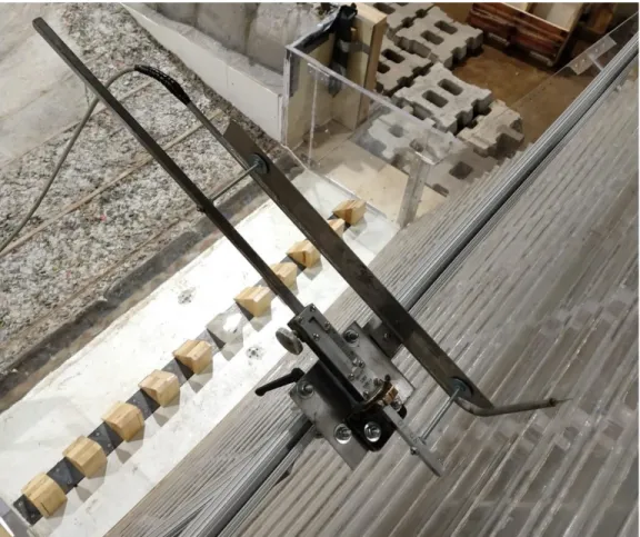
Figure 3.3. The conductivity probe positioned at step 87 near the right sidewall. Step 87 corresponded with the cross-section where flow aeration had spread laterally across the entire chute. ... 30
Figure 3.4. A view of the point-gage assembly attached to the structural frame near the left sidewall of step 38 ... 33
Figure 4.1. A definition sketch of air concentration and velocity profiles for skimming flow over the steps, as viewed from the right side of the chute. ... 35
Figure 4.3. The conductivity probe positioned along the centerline of the chute at elevation Y=0 ... 37 Figure 4.4. The upstream encroachment of the probe’s tips near the chute’s right sidewall, when the point-gage assembly was setup in accordance with the chute-centerline position (see Figure 4.3) ... 38 Figure 4.5. A definition sketch of the lateral position, b, when viewed looking downstream along the chute ... 39 Figure 4.6. The model spillway conveying the design discharge, viewed from a distance ... 41 Figure 4.7. A comparison of streamwise profiles of air concentration measured as the chute conveyed the design discharge, at chute positions: (a) b/B = 0.02, and (b) b/B = 0.50. ... 44 Figure 4.8. Sidewall profiles of air concentration measured between steps 87 and 23 when the chute conveyed the design discharge: (a) dimensional values, and (b) non-dimensional values. 47 Figure 4.9. The longitudinal variations of Y0.90 and Yw near the right chute sidewall when the
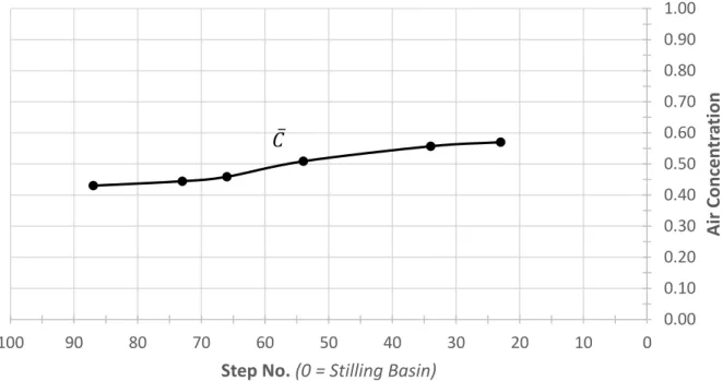
chute conveyed the design discharge. ... 48 Figure 4.10. The longitudinal variations of 𝐶 near the right chute sidewall when the chute
conveyed the design discharge... 49 Figure 4.11. Air-concentration profiles measured for various water discharges at the chute-sidewall position of step 23: (a) dimensional values, and (b) non-dimensional values. ... 52 Figure 4.12. Values of depth-averaged air concentration, measured at the chute-sidewall position of step 23, plotted as a function of water discharge. ... 53 Figure 4.13. Air-concentration profiles at various water discharges, measured at the chute-centerline position of step 23: (a) dimensional values, and (b) non-dimensional values. ... 55 Figure 4.14. Values of depth-averaged air concentration, measured at the chute-centerline
position of step 23, plotted as a function of water discharge. ... 56 Figure 4.15. A definition sketch of the non-dimensional chute positions, b/B ... 57 Figure 4.16. The lateral variations across step 23 of Y0.90 and Ywwhen the chute conveyed the
design discharge; (a) w/o curvature, and (b) w/ curvature. ... 58 Figure 4.17. A scatter plot of air-concentration profiles collected across step 23 when the chute conveyed the design discharge... 59 Figure 4.18. A comparison of air-concentration profiles at/near the chute sidewall (showing negligible influence of sidewall boundary layer on measured values of air concentration). ... 62
Figure 4.19. Time-series of C at the chute-sidewall position, b/B = 0.02, at the approximate flow depth Y0.90 when the chute conveyed its design discharge. In (a): Tw = 1.0 sec and 𝜎𝐶 = 1.9%; in
(b): Tw = 10.0 sec and 𝜎𝐶 = 0.1%. ... 68
Figure 4.20. Time-series of C at chute position b/B = 0.33 when the chute conveyed the roll-wave discharge, Q = 0.021 m3/s. For each value Tw, the standard deviations of the time-series is
assessed, and are as follow: (a) Tw = 10.0 sec, 𝜎<0.5%; (b) Tw = 1.0 sec, 𝜎=2.0%; (c) Tw = 0.8
sec, 𝜎 =2.3%; (d) Tw = 0.4 sec, 𝜎=3.8%; (e) Tw = 0.2 sec, 𝜎=6.3%; (f) 0.1 sec, 𝜎=10.3%. ... 72
Figure 4.21. Velocity profiles measured along the right sidewall when the chute conveyed its design discharge, with values expressed: (a) dimensionally, and (b) non-dimensionally. ... 75 Figure 4.22. Non-dimensional velocity profiles measured for various water discharges at the chute-sidewall position of step 23. ... 77 Figure 4.23. Variations with water discharge of N at the chute-sidewall position of step 23. ... 78 Figure 4.24. Non-dimensional profiles of bulk-flow velocity for various water discharges at the chute-centerline position of step 23. ... 79 Figure 4.25. Variations with water discharge of N at the chute-centerline position of step 23. ... 80 Figure 4.26. A scatter plot of the profile data pertaining to bulk-flow velocity, collected across step 23 when the chute conveyed its design discharge. Values of the bulk-flow velocity are expressed: (a) dimensionally, and (b) non-dimensionally. ... 82 Figure 4.27. A comparison of the measured data pertaining to bulk-flow velocity (Figure 4.26) with the best-fit power functions N = 5 and 7. ... 84 Figure 4.28. A comparison of the measured bulk-flow velocity profile and best-correlated power function for the chute position b/B = 0.02 when the spillway conveyed its design discharge. Exponent N = 4.2, R2 = 0.94. ... 85 Figure 4.29. A comparison of the measured profile of bulk-flow velocity and the best-correlated power function for the chute position b/B = 0.29 when the chute conveyed its design discharge. Exponent N = 8.1, R2 = 0.91. ... 86 Figure 4.30. The distribution of the Darcy-Weisbach friction factor across the chute when the design discharge was conveyed. ... 87 Figure 4.31. A comparison of a typical air-concentration profile measured at the chute position b/B = 0.21, where 𝐶 =0.608 at the chute’s design discharge, with proposed distributions by Wood (1984), Chanson & Toombes (2002) and Takahashi & Ohtsu (2012). ... 88
Figure 4.32. A comparison of a typical air-concentration profile measured at the chute-sidewall position, b/B = 0.50, where 𝐶 = 0.555 at the chute’s design discharge, with proposed
distributions by Wood (1984), Chanson & Toombes (2002) and Takahashi & Ohtsu (2012). .... 89 Figure 4.33. A comparison of 𝐶 as a function of water discharge, with data from the present study (𝜃=63.4o), Straub & Anderson (𝜃=60.0o) and Chamani & Rajaratnam (𝜃=59.0o). ... 91 Figure 4.34. A comparison of measured values of 𝐶 with predicted values of 𝐶, as functions of the chute slope. The data shown are from the present study (𝜃=63.4o), Straub & Anderson (𝜃=60.0o) and Chamani & Rajaratnam (𝜃=59.0o); compared with existing relationships by Hager (1991), Christodolou (1999) and Takahashi & Ohtsu (2012). ... 92 Figure 4.35. A comparison of the values of N calculated for a range of water discharges
measured at two chute positions across 23, with empirical relationship from Takahashi & Ohtsu (2012). ... 94 Figure 4.36. A comparison of the measured bulk-flow velocity profiles collected at the chute-centerline position of step 23 for a range of water discharges, with the predicted profile exponent N = 3.5 from Takahashi & Ohtsu (2012). ... 94 Figure 4.37. A comparison of the calculated values of f from the profile data measured across step 23 when the chute conveyed its design discharge, with predicted value by Takahashi & Ohtsu (2012) and Chamani & Rajaratnam (1999). ... 95 Figure 4.38. Flow separation around a pier by Calitz (2015). In (a), a photograph of the flow separation, and in (b), an iso-contour plot of depth-averaged values of air concentration taken along the chute. ... 97
LIST OF SYMBOLS
𝜃 angle of chute inclination with respect to the horizontal 𝛿 boundary-layer thickness
𝛾 specific weight of water
𝜏 bed-shear stress
𝜌 density of water
𝜈 kinematic viscosity of water 𝜎 surface tension of water
b chute position measured from right sidewall B local chute width (from left to right sidewall) C volumetric air concentration
𝐶̅ depth-averaged air concentration
𝐶̅𝑒 depth-averaged, equilibrium air concentration dc critical flow depth
f Darcy-Weisbach friction factor F* roughness Froude number
Fr Froude number
g gravitational acceleration h vertical step dimension ks step roughness height
l horizontal step dimension
Lr length-dimension ratio of prototype to model scale
Re Reynold’s number
q unit discharge
Q volumetric discharge
Tw a sub-interval over which data are averaged
V bulk-flow velocity
Vw equivalent clear-water flow velocity
Q volumetric discharge
We Weber number
x longitudinal downstream distance from the crest Y flow depth measured normal to the chute invert Yc critical flow depth
Yw equivalent clear-water flow depth
Y0.90 the flow depth where C = 90%
1
INTRODUCTION
1.1
Motivation
This thesis concerns the hydraulic and air-entrainment performance of a unique, ungated stepped spillway. The performance was determined using a hydraulic model constructed at length scale (prototype length/model length) of 24. The new stepped spillway is part of the Gross Reservoir Expansion (GRE) project, which by 2025 is expected to raise the existing Gross Dam about a third of its current height.
The hydraulic model presented a unique opportunity to evaluate the characteristics of flow aeration and energy dissipation along a large-scale, stepped chute of unique geometry. The stepped spillway, which will be the tallest stepped structure in the United States (Ettema et al., 2019), consists of a chute whose step dimensions at model scale, vertical to horizontal, were 0.051 m by 0.025 m, resulting in a chute slope (V:H) of 2.0, and a corresponding chute angle of 63.4o. Additionally, the chute conformed, in planform, to the curved planform of raised Gross Dam. At the spillway’s crest, that radius of curvature was 22.2 m (model scale). Also, the chute’s sidewalls converged at an angle of 2.2o from the top of the chute to the stilling basin at the base of the chute. The chute’s steepness, height, curvature and convergence make the chute’s geometry unique among existing stepped spillways.
1.2
Objectives of Thesis
The set of objectives for this thesis was as follows:
1. Determine how the concentration of flow-entrained air varied along and across the spillway’s chute. This objective had several specific objectives:
a) Evaluate (for the chute’s design discharge) the streamwise variations of air concentration within a region of the chute where flow transitioned from gradually varied (i.e. actively bulking) to nominally equilibrium;
b) Measure in a section of nominally equilibrium flow near the right sidewall and along the chute centerline, the variations of air concentration for water discharges less than the design discharge;
c) Ascertain the effects of chute curvature on air concentration;
d) Assess for the chute’s design discharge the lateral variations of air concentration across the chute; and relatedly, the water surface, defined in this study as Y0.90, the
flow depth where C = 0.90;
e) Ascertain the effects of chute convergence on air concentration along the chute; and,
f) Examine what a time-series of air concentration fluctuations looks like, both for the design discharge and for a low discharge where roll waves were present along the chute.
2. Obtain profiles of bulk-flow velocity throughout the chute. This objective had several specific objectives:
a) Evaluate (for the spillway’s design discharge) the streamwise variations of bulk-flow velocity along the right descending sidewall of the chute; and,
b) Ascertain what effect the chute curvature had on the measured flow-velocity distributions.
1.3
Background
Gross Dam, owned and operated by Denver Water and built in 1954, is an existing concrete gravity-arch dam located in Boulder County, Colorado. As presently constructed, the dam impounds the South Boulder Creek to a water-surface elevation that is 103.6 m above the natural stream bed (with a water-storage volume of about 51.8 million cubic meters). Figure 1.1 shows the current lay of the reservoir and dam.
1.4
Gross Reservoir Expansion
The Gross Dam Expansion (GRE) Project will raise the existing Gross Dam by 40.0 m to an ultimate height of 143.6 m, thereby increasing the water-storage capacity to about 146.8 million cubic meters. The raised dam will be a thick-arch type of dam and will be constructed using roller-compacted concrete (RCC). The face of the structure will be laid using conventionally vibrated concrete (CVC).
Figure 1.2: A comparison of the existing Gross Dam and proposed Gross Dam. On left, the existing structure with crest elevation of 2221.9 m, and on right, the proposed structure with crest
elevation of 2261.9 m. [https://grossreservoir.org/construction/raising-a-dam/]
With the completion of the GRE, Gross Dam’s new ungated stepped spillway will be the tallest stepped structure in the United States (Ettema et al., 2019). In addition to the spillway’s height, the steepness, length and curved form of the spillway’s chute make the spillway unique. As such, a model study was undertaken by Colorado State University’s Hydraulics Laboratory to
investigate the hydraulic performance of the design.
At model scale, the chute’s nominal step dimensions, vertical to horizontal, were 0.051 m by 0.025 m, resulting in a chute slope (V:H) of 2.0 and angle of 63.4o. The chute was imparted with horizontal curvature, with radius of 22.2 m. The spillway crest featured two piers, each 0.032 m wide, at the one-third points along the crest width. The chute’s sidewalls converged from a width of 2.23 m at the crest to 1.78 m at the stilling basin, a convergence angle of 2.2o. The spillway was designed to convey the watershed’s Probable Maximum Flood (PMF), which at model scale was 0.347 m3/s.
The hydraulic model of the spillway was constructed within the hydraulics laboratory of CSU’s Engineering Research Center (ERC), at a length scale of 24. The model was operated in
accordance with the principle of Froude number similitude. The components of the model are discussed in greater detail in Section 3.2, which includes plan and profile drawings of the model. The model was constructed in order to assess the performance of the overall structure, with particular focus on the flow transition from the crest to the stepped chute (i.e., to verify that jet deflection does not occur); to determine the requisite sidewall height; to evaluate the amount of flow energy dissipated along the chute; to evaluate the performance of the stilling basin design; and to measure pressures throughout the model to check for incipient cavitation. The results of these investigatory objectives can be found within the model study report by Ettema et al. (2019)
1.5
Format of Thesis
The Table of Contents lists the format of this thesis. In brief, this thesis includes the following features: in Chapter 2, a review of literature related to aeration, stepped spillway hydraulics and similitude principles; in Chapter 3, an overview of the hydraulic model, the measurements obtained throughout the chute, and the instrumentation used; in Chapter 4, a presentation of the results pursuant to the objectives of the thesis (Section 1.2), with discussions and analyses; and, in Chapter 5, concluding remarks and thoughts regarding future work.
2
LITERATURE REVIEW
2.1
Introduction
In recent decades, extensive amounts of experimental studies have been undertaken to evaluate the characteristics of aerated flows along stepped chutes. Such evaluations have typically been in terms of measured values of air concentration and water surface, bulk-flow velocity, pressure, and overall energy dissipation along the chute. From those studies, guidelines have been formulated to aid in the design of stepped chutes (e.g., Chanson, 2001; Boes & Hager, 2003b; Frizell & Frizell, 2015). This chapter reviews the extant literature regarding the various aspects of air entrainment by water flows down spillway chutes. Included in the review are suggested scale limits for laboratory models of water and air flow down chutes.
A knowledge gap still exists for the influences on air entrainment of certain geometric features of chutes. As noted in the literature (Geringer & Officer 1995, Matos & Meireles 2014), chute curvature and its effects on air-water flows within stepped chutes are issues requiring further investigation. To date, no experimental study has evaluated those effects, in large part because of economic considerations. For example, Wolwedans Dam in South Africa is a gravity-arch type of dam, whose spillway conforms to the planform curvature of the dam; the spillway chute of Wolwedans Dam is nearly identical in design to the new spillway for Gross Dam. However, in the hydraulic-model study that was undertaken to assess that spillway’s design, the chute model was constructed to be prismatic (i.e., without the feature of planform curvature) so that the chute model could be repurposed for later investigations (van Staden, 1991). Given the large number of gravity-arch dams which have been constructed, and the emergent trend of raising existing dams for additional water-storage capacity, knowledge of the effects of chute curvature on air-water flows should be determined.
Also, most experimental studies of stepped spillways have featured chutes whose slopes were equal to or less than the slope typical of RCC dams (𝜃 = 53.1o, or chute slope = 1.33). While there are some notable exceptions (e.g., Straub & Anderson, 1958; van Staden, 1991; Chamani & Rajaratnam, 1999; Ohtsu, Yasuda & Takahashi, 2004; Takahashi & Ohtsu, 2012), data
concerning steep, stepped chutes are scant and have not been incorporated into many of the existing, empirical relationships found in the literature.
Figure 2.1 is a plot of flow regimes, taken from a design guideline by the USBR. Along the abscissa, the ratio h/l represents, for a given chute, the ratio of the steps’ riser and tread
dimensions (i.e., the chute slope). Gross Dam, whose chute slope is 2.0, lies beyond the plotted data, and even beyond the figure’s margins.
Figure 2.1: A plot of stepped chute flow regimes, with experimental data sources given in the legend (Frizell & Frizell, 2015). Along the ordinate, dc refers to the critical flow depth, herein
referred to as Yc.
This literature review outlines the key measurements typically undertaken to evaluate aerated flows along stepped chutes. In the present thesis, those measurements are used to assess the flow, and to ascertain the effect of the chute’s curvature on flow within the chute. Included in this review are pertinent, empirical relationships from the literature. Yet, most relationships (formulated for lesser chute slopes) do not conform to the data obtained along the steep chute model of Gross Dam spillway.
2.2
Air Entrainment and Concentration
The entrainment of air is a common occurrence in turbulent, open-channel flows. Along steep spillway chutes, air entrainment is a prominent feature of the flow. Air entrainment occurs when
the thickness of the turbulent boundary layer (𝛿) of water flow extends to the free surface. When that condition is met, the forces associated with water’s surface tension and air-bubble buoyancy are overcome, and air can be entrained into the water column (Chanson, 1995).
The process of air entrainment in a stepped spillway depends on several factors, e.g., step dimensions and corresponding roughness along a stepped chute’s invert, the boundary layer along a chute’s sidewall, and the presence of flow obstructions that induce turbulence in flow down a spillway; notably, bridge piers along a spillway’s crest.
Air concentration, C, is a measure of the volume of air per unit volume of total discharge. In air-water flows, air concentration is typically measured intrusively from an Eulerian perspective by analyzing the instantaneous void fraction through time at a fixed point location (Felder & Chanson, 2015). By measuring air concentration at successive flow depths and streamwise locations, the distribution of C and representative flow depths can be defined for a spillway. A representative flow depth relates to a prescribed value of air concentration. It is common practice (e.g., Straub & Anderson, 1958) to relate flow depth to a prescribed value of C. The water surface of skimming flow1 along a spillway chute is commonly taken to be Y0.90; i.e. Y at
which C = 0.90. This flow depth has been found to satisfy continuity analyses for air-water mixtures (Wood, 1991). Up to a flow depth of Y0.95, the mixture is said to be quasi-homogenous
wherein the slip velocity between the water surface and the air surface is negligible (Chanson, 2013).
From a measured profile of air concentration, the depth-averaged value of air concentration, 𝐶̅, is obtained as: 𝐶̅ =𝑌1 0.90∫ 𝐶 𝑑𝑦 𝑦=𝑌0.90 𝑦=0 (2.1) A similar integral calculation yields 𝑌𝑤, the equivalent clear-water flow depth. This theoretical value of flow depth omits all entrained air from the water-column; i.e.,
1 Appendix B gives further details regarding the flow regimes of stepped chutes (skimming, nappe and transition
𝑌𝑤 =𝑌0.901 ∫𝑦=0𝑦=𝑌0.90(1 − 𝐶) 𝑑𝑦 (2.2) From Eq. 2.1 and Eq. 2.2, Yw also can be calculated as:
𝑌𝑤 = 𝑌0.90(1 − 𝐶̅) (2.3)
Just as flow depth can be expressed in terms of the bulk value of the air-water mixture (Y0.90) and
a clear-water equivalent (Yw), so too can flow velocity be expressed in terms of the measured,
bulk value of the mixture (V) and a clear-water equivalent (Vw).
From continuity, the clear-water flow velocity can be calculated, for a prismatic channel, by the following expression:
𝑉𝑤 = 𝑞𝑌𝑤𝑤 , (2.4)
where qw is the unit-water discharge.
The bulk-flow velocity is measured using a dual-tip conductivity probe. The values are obtained by performing a cross-correlation analysis on two voltage time-series, measured simultaneously at an offset distance in 𝑥 (the streamwise coordinate). The cross-correlation analysis (Section 3.4.2) yields the travel time of the mixture, t, which is then used to calculate the bulk-flow velocity using the known offset in 𝑥 (i.e., 𝑉 = 𝑥/𝑡).
In many applications (e.g., calculating the Darcy-Weisbach friction factor coefficient), clear-water parameters (both of flow depth and velocity) are used in lieu of the bulk-flow parameters.
2.3
Friction Factor
In skimming flows, form drag is the primary mechanism of energy dissipation (Chanson, 2006). Commonly, such energy dissipation is expressed in terms of the Darcy-Weisbach friction factor coefficient, f, calculated using Eq. 2.5, which uses the clear-water flow parameters:
𝜏𝑜 = 𝛾 𝑌𝑤 sin 𝜃 = 𝑓8𝜌𝑤𝑉𝑤2, (2.5)
where 𝛾 is the specific weight of water and 𝜌 is the density of water. The friction factor is alternatively given by Takahashi & Ohtsu (2012) as
𝑓 = 8 (𝑌𝑤
𝑌𝑐)
3
The Darcy-Weisbach friction factor has been found to be independent of chute slope for 𝜃 < 12o (Chanson, 1994; Chamani & Rajaratnam, 1999). For 𝜃 > 25o, a large amount of scatter is noted within experimental data (Christodoulou, 1999).
Prior to the assemblage of empirical data sets along steep, stepped chutes, Chanson (1995) suggested f ~ 1 as an order-of-magnitude approximation. Shortly thereafter, Chamani &
Rajaratnam (1999) provided the following expression, based on experimental data for 50o < 𝜃 < 60o:
1
√𝑓 = 2.16 + 1.24 log ( 𝑦
𝑘𝑠) (2.7)
Matos (1999) and Matos & Meireles (2014) suggest that f is a function of water discharge in steep, stepped chutes, because the overall flow resistance reduces in consequence of drag reduction with increasing discharge. This point is discussed by Boes & Hager (2003b). Figure 2.2 shows that, in steep stepped spillways, f ~ 1 is not a good approximation, as data show values of f as low as 0.05:
Figure 2.2. Reduction in f with increase in Yc/h for 𝜃=53.1o (Matos & Meireles, 2014).
Takahashi & Ohtsu (2012) give the following regression equation for 19o < 𝜃 < 55o to calculate the effective f along a stepped channel as a function of 𝜃, S and the smooth-chute equivalent f.
𝑓 = [−9.2 𝜃 ∗ 10−4+ 0.12] tanh(4𝑆) + 𝑓
𝑠𝑚𝑜𝑜𝑡ℎ (2.8)
where S = h/Yc and fsmooth = 3.8𝜃2∗ 10−5− 4.4𝜃 ∗ 10−3+ 0.135.
2.4
Equilibrium Flow Conditions
The chute of a stepped spillway conveying a skimming flow may attain equilibrium conditions of flow, whereupon the measured values of air concentration and water surface become step
invariant. The literature reports that values of equilibrium, depth-averaged air concentration (𝐶̅𝑒) are not affected by chute roughness (Ruff & Frizell, 1994; Chanson, 1994; Boes & Hager, 2003b; Matos & Meireles, 2014). Further, the prevailing notion is that equilibrium air content is not affected by the magnitude of water discharge, but by chute slope only. Hager (1991) gives the following relationship for 𝐶̅𝑒 as a function of chute slope:
𝐶̅𝑒 = 0.75(sin 𝜃)0.75 (2.9)
Christodoulou (1999) gives a similar expression, which predicts higher values:
𝐶̅𝑒 = 0.9 sin 𝜃 (2.10)
The basis of Hager & Christodoulou’s formulations is the air concentration data collected by Straub & Anderson (1958), who used a variable-slope, smooth-invert chute artificially roughened with sand. The measure of flow uniformity adopted by Straub & Anderson was
successive equality of air-concentration profiles measured streamwise along the chute. When that condition of equality was met, they considered the flow to be in equilibrium. Hence their
measured value of 𝐶̅ was taken to be the equilibrium value for that configuration of slope and water discharge.
The results of their measurements showed that 𝐶̅𝑒 was constant at low water discharges, but, for steep chutes (𝜃 > 30o), 𝐶̅𝑒 began to decrease with increasing discharge. Accordingly, from their data, Straub & Anderson produced a relationship for 𝐶̅ that is dependent on slope and discharge: 𝐶̅ = f(S, q1/5), where S = tan(𝜃).
While Straub & Anderson considered every one of their measurements to have met this equality condition, Wood (1983) later argued that equilibrium flow conditions may not have been attained for some of their measurements. Figure 2.3 was produced by Wood, and it plots the data from
Straub & Anderson. Each chute-slope configuration (7.5o, 15o… 60o, 75o) was plotted as a separate contour, 𝐶̅ = f(𝑄). Wood demonstrated his argument by showing a horizontal parabola that delineated a region of constant 𝐶̅𝑒 from a region where 𝐶̅ decreased for a given slope of chute.
Figure 2.3. Conjectured regions of non-equilibrium flow (Wood, 1983, based on data from Straub & Anderson, 1958).
The basis of Wood’s argument is that, all data points to the right of the curve labeled “region of non-equilibrium flow” must have been measured in gradually varied flow; because, for each chute-slope configuration, 𝐶̅ should be constant for every water discharge, as suggested by the trend of constant 𝐶̅ for water discharges which fall to the left of the curve.
However, later researchers’ findings seem to agree with Straub & Anderson; e.g., the data set collected by Chamani & Rajaratnam (1999) on a chute with 𝜃=53.1o (chute slope = 1.33) and 59.0o (chute slope = 1.66). Chamani and Rajaratnam characterize the flow region at the bottom of their chute as being a “region of fully developed (skimming) flow” – and in this region, 𝐶̅ consistently decreased with increasing Q. Figure 2.4 shows a plot of their data, where 𝐶̅ = f(𝑄) in a similar fashion to the trend in Figure 2.3.
A useful comparison is to apply the equation proposed by Hager to the spillway used by Chamani & Rajaratnam. The comparison gives 𝐶̅𝑒(𝜃=53.1o) = 0.634, and 𝐶̅𝑒(𝜃=59.0o) = 0.668. Similarly, applying the equation by Christodoulou gives 𝐶̅𝑒(𝜃=53.1o) = 0.720, and 𝐶̅𝑒(𝜃=59.0o) = 0.771.
Figure 2.4. 𝐶̅𝑒 as function of Q for 𝜃 = 59o (Chamani & Rajaratnam, 1999). Accordingly, Chamani & Rajaratnam saw fit to include in their regression equation the
parameter of unit-water discharge. The resulting equation is similar to that produced by Straub & Anderson:
𝐶̅𝑒= 0.93 log ((sin 𝜃)
0.1
𝑞0.3 ) + 1.05 (2.11)
Similarly, Ohtsu, Yasuda & Takahasi (2004) observe the influence of water discharge on 𝐶̅𝑒. These authors, rather than dichotomizing skimming flow as being either equilibrium or non-equilibrium, consider the flow as being either quasi-uniform (developed) or non-quasi-uniform (developing). They give a relationship for 𝐶̅𝑒 in quasi-uniform flow as a function of the
reciprocal of Yc/h:
𝐶̅𝑒 = 𝐷 − 0.30 exp (−5 (𝑌ℎ𝑐) 2
− 4𝑌ℎ
𝑐) , (2.12)
where D = 0.300 for 5.7o < 𝜃 < 19o, and D = -2.0*10-4*θ2 + 2.14*10-2*θ – 3.57*10-2 for 19o < 𝜃 < 55o.
𝐶̅𝑒= (6.9𝜃 − 0.12) 𝑆 + 0.656{1 − exp[−0.0356 (𝜃 − 10.9)]} + 0.073 , (2.13) where S= Yc/h, valid for 19o < 𝜃 < 55o.
Boes & Hager (2003a) note the use of three approaches to confirm uniform flow conditions. The first approach, used by Straub & Anderson (also Chamani & Rajaratnam, and others), is to compare profiles of air concentration measured at successive cross-sections to show equality. A second approach is to examine the longitudinal water-surface profiles of both Yw and Y0.90. The
third approach is to calculate the friction factor, wherein Yw is raised to third power (𝑓 =
8 (𝑌𝑤
𝑌𝑐)
3
sin 𝜃), thereby causing deviations to be more pronounced.
The data collected in the Gross Dam stepped spillway (Section 4.3.3) agrees with the findings of Straub & Anderson; Chamani & Rajaratnam; Ohtsu, Yasuda & Yakahasi, and others – that 𝐶̅𝑒 is in fact influenced by water discharge.
2.5
Vertical Distribution of Air Concentration
The vertical distribution of air concentration has been described in both developing and equilibrium flow regions by numerous models. Wood (1984) formulated the following
distribution, intended for smooth-invert chutes (although it works suitably well when applied to stepped spillways, because air concentration is not a function of chute roughness (Ruff & Frizell, 1994)):
𝐶 = 𝐵′ (𝐵′+ exp[−𝐺′cos 𝜃∗ ( 𝑌
𝑌0.90)
2])
⁄ , (2.14)
where the coefficients are given in Table 2.1, from Chanson (1993) based on re-analysis of data by Straub & Anderson (1958):
Table 2.1. Coefficients for Wood’s distribution (Chanson, 1993).
𝜃 𝐶̅ 𝐺′cos 𝜃 𝐵′
37.5 0.569 2.675 0.6203
45.0 0.622 2.401 0.8157
60.0 0.680 1.894 1.354
75.0 0.721 1.574 1.864
Chanson & Toombes (2002) provide an alternative model, based on the bubble-diffusion equation: 𝐶 = 1 − tanh (𝑘′− 𝑌 𝑌0.90 2∗𝐷𝑜 + [𝑌0.90 𝑌 −1 3⁄ ]3 3∗𝐷𝑜 ) 2 , (2.15)
where the integration constants k’ is given by Eq. 2.17, from Do which is solved for iteratively
using Eq. 2.16 and a known value of 𝐶̅:
𝐶̅ = 0.7622{1.0434 − exp(−3.614∗𝐷𝑜)} (2.16) 𝑘′ = atanh(√0.1) + 1
2∗𝐷𝑜− 8
81∗𝐷𝑜 (2.17)
Takahashi & Ohtsu (2012) give a simplified form of the bubble-diffusion equation:
𝐶 = 1 − tanh (𝑘′− 𝑌 𝑌0.90 2∗𝐷′) 2 (2.18) 𝑘′ = atanh(√0.1) + 1 2∗𝐷′ (2.19) 𝐷′ = (0.848 𝐶̅ − 0.00302) (1 + 1.1375 𝐶̅ − 2.2925 𝐶̅⁄ 2) (2.20)
2.6
Longitudinal Development of Air Concentration
The development of 𝐶̅ as a function of x (the longitudinal distance from the spillway crest) is chute specific, and depends on the slope, and possibly water discharge. A common approach to expressing 𝐶̅(𝑥) is in terms of the height relative to the spillway crest, Hd, defined positive in -𝑧̂;
normalized by the critical flow depth. The following figure from Matos & Quintela (1995) shows empirical data for 𝜃=53.1o assembled in this form:
Figure 2.5. 𝐶̅ as function of Hd/Yc (Matos & Quintela, 1995).
For 𝜃 = 53.1o (typical of RCC dams), Matos (2000) gives the following equation to predict 𝐶̅(𝑥): 𝐶̅ = 0.210 + 0.297 exp{−0.497(ln 𝑠′− 2.972)2} (2.21)
𝐶̅ = (0.888 −1.065√𝑠′ )2 (2.22)
Here, the normalized parameters 𝑠′=𝑥−𝐿𝑖
𝑍𝑖 and 𝑍𝑖 =
𝑧−𝑧𝑖
ℎ𝑐 . The first equation is intended for 0 < s’
< 30 and the second for s’ > 30.
Boes & Hager (2003a) present an alternative equation for 26o < 𝜃 < 55o, where air concentration is expressed in a normalized form, ci:
𝑐𝑖 = [𝐶̅(𝑍𝑖) − 𝐶̅𝑖] (𝐶̅⁄ 𝑒− 𝐶̅𝑖) (2.23) 𝑐𝑖 = [tanh (5𝑥10−4(100° − 𝜃)𝑍𝑖]1/3 (2.24) Here, 𝐶̅𝑖 is the mean air concentration at some point downstream the incipient point of aeration; 𝐶̅(𝑍𝑖) is the mean air concentration at the point of incipience; and 𝑍𝑖 is the elevation below the spillway crest of incipience. The uniform value 𝐶̅𝑒 is calculated from the expression by Hager (1991).
Figure 2.6. Normalized air-concentration distribution C(Y*) for 𝜃 = 50°, Fo = 3.5, K = 20 mm
and ho/s = 1.06 (Boes & Hager, 2003a).
Boes & Hager (2003b) give an expression for the height below the spillway crest where uniform flow conditions are attained.:
𝐻𝑑𝑎𝑚,𝑢
𝑌𝑐 = 25.52[1 − 0.055(sin 𝜃)
−1/3](sin 𝜃)2/3 (2.25)
Here, the subscript u refers to “uniform” and is synonymous with the subscript e implying equilibrium.
Meireles et al. (2007) present plots of 𝐶̅ as a function of x (expressed in terms of step no.) for 𝜃 = 53.1o, for different values of 𝜓, where 𝜓 is the characteristic flow depth at which the water surface is defined: 0.90, 0.95, or 0.99. For each characteristic flow depth, 𝐶̅ is evaluated for two sets of flow conditions: on left, h = 4 cm and qw = 0.080 m2/s; and on right, h = 8 cm and qw =
Figure 2.7. 𝐶̅(𝑥) for 𝜃 = 53.1o (Meireles et al., 2007)
In Figure 2.8 (Meireles et al. 2007) the bulk flow depth is shown for each value of 𝜓, and the respective trends (within each plot) are independent of 𝜓 (flow conditions are the same as for Figure 2.7).
Figure 2.8. 𝑌𝜓(𝑥) and 𝑑𝜓(𝑥) for 𝜃 = 53.1o (from Meireles et al., 2007) Here, the clear-water flow depth Yw is expressed as dψ.
Similar to Figure 2.8, Figure 2.9 from Matos & Meireles (2014) shows 𝐶̅ as function of x (step number) for additional flowrates (for the same spillway slope):
Figure 2.9. 𝐶̅(𝑥) for various values of Yc/h for 𝜃 = 53.1o (Matos & Meireles, 2014)
When normalized in x as (L-Li)/di, as in Figure 2.10, 𝐶̅ varies rapidly downstream the inception
point, then, for some flow conditions, is seen to rooster-tail as the flow transitions into to gradually-varied.
Figure 2.10. 𝐶̅(𝑥) for Yc/h = 1.1 & 2.0, 𝜃 = 53.1o (Matos & Meireles, 2014).
2.7
Bulk-Flow Velocity
The velocity distribution of aerated, skimming flows has been found to be approximated by a power-law function up to 80% of the flow depth Y0.90, above which the magnitude of the
bulk-flow velocity is constant (Boes & Hager, 2003a). The general form of the power-law function is 𝑉 𝑉0.90 = 𝑎 ( 𝑌 𝑌0.90) 1/𝑁 for 𝑌𝑌 0.90 < 0.8 (2.26) 𝑉 𝑉0.90= 1 for 𝑌 𝑌0.90> 0.8 (2.27)
These equations include an exponent N and a scalar a, though a is generally close to unity and is frequently omitted in the literature.
Boes & Hager (2003a) evaluated a number of experimental data sets and found the coefficients are best approximated as a = 1.05 and N = 4.3 for 26o < 𝜃 < 55o. For flatter slopes, they note that N generally increases. Yasuda & Chanson (2003) found that N = 9 for 𝜃 = 15.6o.
Boes & Hager (2003a) further state that to model the velocity distribution of skimming flow without scale effects the limiting values of Re and We are Re >105 and We >100. In their study,
they found that N was unaffected by chute slope or water discharge within the range of slopes that they tested.
On the whole, a large amount of scatter exists among values of N reported by different researchers, ranging from N = 3.5 by Chanson (1994), to N = 6.3 by Cain (1978), to, as previously cited, as high as N = 9 by Chanson & Yasuda (2003). The reference by Andre, Boillat, & Schleiss (2004) provides a review of additional, discrepant values of N from various researchers, and the flow conditions and chute configurations for which they were collected. Takahashi & Ohtsu (2012) give a regression equation for the exponent of the form:
𝑁 = 14𝜃−0.65𝑆 (100
𝜃 𝑆 − 1) − 0.041𝜃 + 6.27 (2.28)
where S = h/Yc, and for 19o < 𝜃 < 55o.
2.8
Sidewall Height
When flow along a spillway chute becomes aerated, the flow depth bulks. For the design
engineer, quantifying the degree of bulking is an important consideration because it dictates how high the chute sidewalls must be to contain the flow.
Many design guidelines have suggested that a safety factor η can be applied to Y0.90, yielding the
design height of sidewall. Boes & Hager (2003b) suggest η = 1.2 for concrete dams and η = 1.5 for embankment dams. A different value of η = 1.4 is suggested by Ohtsu et al. (2004), informed by the measured ratio of characteristic flow depths Y0.99/Y0.90.
Following the same approach as Ohtsu et al., Meireles et al. (2007) examined the ratios Y0.95/Y0.90
and Y0.99/Y0.90 as functions of Yc/h for stepped chutes with slopes typical of RCC dams (i.e.
𝜃=53.1o), and found an inverse relationship given by the following expressions: 𝜂 = (𝑌0.95 𝑌0.90)𝑚𝑎𝑥 = 1.061 + 0.1322 ( 𝑌𝑐 ℎ) −1.034 (2.29) 𝜂 = (𝑌0.99 𝑌0.90)𝑚𝑎𝑥 = 1.140 + 0.8143 ( 𝑌𝑐 ℎ) −1.499 , (2.30)
2.9
Similarity
In the design and operation of hydraulic models, similarity considerations set the proportions of lengths and forces between prototype and model-scale values.
Geometric similarity describes the ratio of lengths between the prototype structure and the model structure. If Lrrepresents that ratio of Lp/Lmwhere p refers to prototype and m refers to model,
then the scale factor is defined as 1:Lr. For example, the Gross Dam hydraulic model was
constructed at a length scale Lr= 24, which corresponds with a scale factor of 1:24.
Kinematic similarity describes the proportions of motion between prototype and model,
expressed in terms of velocity and acceleration. To achieve kinematic similarity, the velocity at model-scale should be proportional to the velocity at prototype-scale in the same homologous location; and, that same proportionality should hold for the ratio of accelerations. By maintaining kinematic similarity, the flow behavior in the model, in terms of velocity and acceleration, replicates exactly the behavior at prototype scale.
Dynamic similarity describes the ratio of forces between prototype and model. Typically, water flowing in an open-channel experiences three forces: gravity, viscosity, and surface tension. To maintain dynamic similitude in a hydraulic model, the forces of gravity, viscosity, and surface tension are evaluated in terms of three dimensionless numbers:
• The Froude number, which represents the ratio of inertia to gravity: o 𝐹𝑟 = √𝑔 𝑌𝑉
• The Reynolds number, which represents the ratio of inertia to viscosity: o 𝑅𝑒 = 𝑉 𝑌𝜈
• The Weber number, which represents the ratio of inertia to surface tension: o 𝑊𝑒 = 𝜌𝑉𝜎2𝐿
For true dynamic similarity between the prototype and model structures, the ratios of all three dimensionless numbers must be equal – i.e., (𝐹𝑟)𝑝
(𝐹𝑟)𝑚 =
(𝑅𝑒)𝑝
(𝑅𝑒)𝑚=
(𝑊𝑒)𝑝
(𝑊𝑒)𝑚. Yet, simultaneous similarity
of all three dimensionless numbers is not realistic between prototype and model scale (Boes & Hager, 2003). Therefore, a common approach in the design of hydraulic models which simulate
open-channel flow processes is to maintain only similarity of the Froude number. But, because similarity is not strictly enforced for the Reynolds and Weber numbers, the modeled proportions of viscosity and surface tension do not reflect exactly the proportions at prototype scale.
Generally, the viscous effects incurred by incomplete similarity of the Reynolds number can be neglected if the flow is fully turbulent at model scale. However, incomplete similarity of the Weber number is problematic in the modeling of two-phase, aerated flows, because unduly high surface tension may affect the physical processes of entrainment and mixing.
2.9.1
Scale Effects
In open-channel flows, the process of air entrainment occurs when surface-tension forces at the free-surface are overcome by turbulence. When that process is simulated in a hydraulic model scaled according to Froude number similitude, the incorrect proportions of viscosity and surface tension induce unavoidable scale effects in the model. These problems, of viscosity and surface tension, owe to incomplete dynamic similitude.
Another consideration in the true replication of air entrainment processes at model scale is the geometric length scale at which the model is constructed. Boes & Hager (2003) state that
because the size of entrained air bubbles cannot be scaled proportionally to the geometric length scale, they are proportionally too large in models where Froude number similitude is used. Thus, at model scale, the transport capacity of entrained air is lower, and the rate of bubble detrainment is higher than they should be.
To limit the scale effects associated with transport and detrainment as described by Boes & Hager, recommendations suggest limits for the geometric length scale. Pinto et al. (1982) showed that a length scale between 10 and 15 is needed to properly model the entrainment of air in free-surface open channel flows. Later research by Boes (2000) confirmed that a length scale of 10 is optimum. It’s noted that, when the length scale is kept within this range, the forces of surface tension and viscosity do not hinder the process of entrainment (Wood, 1991).
However, some hydraulic models cannot be constructed at such a length scale. For example, the Gross Dam stepped spillway was constructed at a length scale of 24, and very nearly does not fit inside the testing hall of CSU’s hydraulics laboratory. In such models, air entrainment may still be correctly modeled by maintaining minimum values of the Reynolds and Weber numbers.
Chanson and Pfister (2013) indicate these limits to be We0.5>140 and Re > 2x10⁵ to 3x10⁵, when
3
EXPERIMENTAL MODEL & METHODOLOGY
3.1
Introduction
This chapter gives information regarding the design and operation of the hydraulic model, which was constructed at a length scale (prototype length/model length) of 24. The model’s dimensions and underlying similitude principles are presented here. Also discussed are the methods whereby data were collected, and the instrumentation used in these methods.
3.1.1
Model Dimensions and Layout
The Gross Dam hydraulic model was constructed in a horizontal-bed, concrete-lined flume of plan dimensions 6.93 m by 30.48 m, and sidewalls 1.00 m high.
Table 3.1 gives the general dimensions of the model. Figure 3.1 and Figure 3.2 show plan and profile drawings of the model’s layout, respectively.
Some key components of the model are as follow:
• The head tank, which simulated a portion of Gross Reservoir centered on the spillway. The head tank had planform dimensions of 4.67 m by 4.67 m, and a depth of 1.52 m. The tank contained a flow-distributor (diffuser) box. The diffuser featured several layers of semi-permeable mesh, through which flow was forced to pass on its approach to the spillway crest. By this means, the flow within the head tank was made to be uniform as it approached the spillway crest.
• The crest, which had an ogee form and featured two piers, spaced at positions of 1/3 and 2/3 of the crest’s width.
• The chute, which was curved and consisted of 118 steps with dimensions (V:H) of 0.051 m by 0.025 m (𝜃 = 63.4o). The chute included a transitional sub-reach immediately downstream the crest, consisting of eleven steps whose dimensions increased until the nominal values were attained. The chute was buttressed by converging sidewalls, which converged at an angle of 2.2o. The model-scale width of the chute was 2.28 m at the crest, and 1.78 m at the entrance of the basin.
• The stilling basin, which was a modified design custom-developed for the spillway (Ettema et al., 2019).
• The sidewalls along the chute had dimensions vertical to the step treads of 0.33 m, which measured normal to the chute invert were 0.14 m in height.
In addition, the hydraulic model was constructed with scaffolding along the length of the spillway. The scaffolding, not shown in the plan or profile drawings but visible in Figure 3.3, was constructed of 80/20 Aluminum, and enabled for close access to the chute during model operation. 80/20 Aluminum was also used to construct a frame which spanned across the chute and supported a point-gage assembly during measurements of air concentration and bulk-flow velocity (Section 3.5.1).
The following table gives noteworthy model dimensions:
Table 3.1. Model dimensions
Model Component Dimensions
Height of ogee crest 5.94 m
Height of bottom of head tank 4.95 m
Chute width at crest 2.23 m
Chute width at stilling basin 1.78 m
Chute angle 63.4o
Step riser 0.051 m
Step tread 0.025 m
Design head over crest 0.169 m
3.2
Similitude and Model Scaling
The hydraulic model was constructed at a length scale of 24, and the model was operated in accordance with the principle of Froude number similitude. Table 3.2 gives various parameters and their model-scale values for the prototype structure.
Table 3.2. Values of variables at model scale
Variable Scale Scale Value
Length Lr 24.0 Velocity Lr1/2 4.9 Discharge Lr5/2 2,821.8 Pressure Lr 24.0 Time Lr1/2 4.9 Frequency Lr-1/2 0.2 Force Lr3 13,824.0 Reynolds No. Lr3/2 117.6 Webers No. Lr2 576.0
3.3
Measurements
Extensive amounts of data were measured throughout the physical model pursuant to the objectives of the model study – in the head tank, stilling basin, terminal tailwater channel, and along the chute. Generally, measurements consisted of flow velocities, both clear-water and air-entrained; air concentrations; water-surface elevations; pressures; flow-streak lines; as well as general, visual assessment of the overall hydraulic performance: e.g., in optimizing the placement of the baffle blocks within the stilling basin.
Data pertaining to air concentration and flow velocity were recorded systematically throughout the spillway, beyond the scope of the GRE model study, specifically to investigate the nature of aeration in the geometrically unique stepped chute.
This section explains where the measurements of air concentration and flow velocity (both measured using the same instrument) were taken along the spillway chute, and for what flow conditions. Also explained are the flow conditions used for the measurements.
3.3.1
Air Concentration
Measurements of air concentration were recorded point-wise and assembled into profiles normal to the chute, for a variety of discharges and in several locations (see Figure 4.1 for a definition sketch of the measured profile orientations).
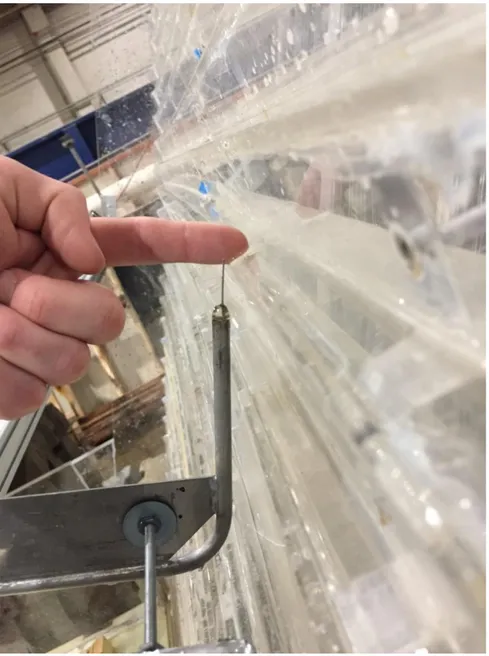
The measurement instrument, a conductivity probe, functioned as a bubble detector when submerged in an air-water mixture. Each sample of air concentration data was collected for a minimum of 30 seconds, some sets for 60 seconds. The probe was affixed to a point gage which let profiles originating from the invert to be measured precisely along the gage’s major divisions at increments of 0.01 ft = 3.05 mm.
Air concentration was used as the basis for defining the water surface (Y0.90) throughout the
chute. Depth-averaging was performed on the measured profiles to obtain the mean values (𝐶̅). From Y0.90 and 𝐶̅, an equivalent value of the clear-water flow depth (Yw)was then calculated.
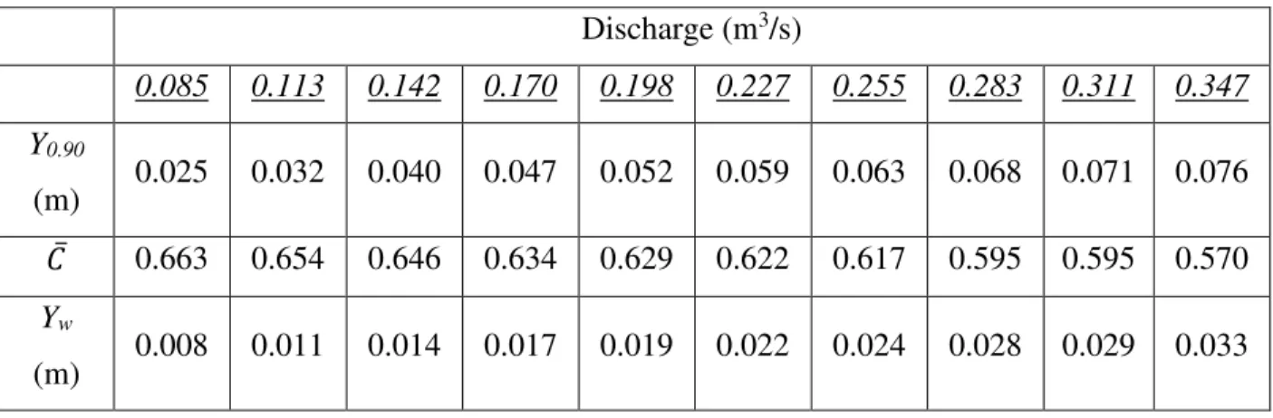
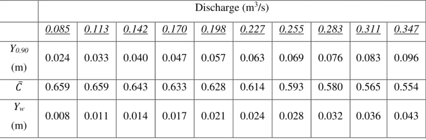
Values of Y0.90, 𝐶̅ and Yw were used to show nominally equilibrium flow conditions at the design
discharge (Q = 0.347 m3/s) by comparing values between an upstream and downstream section of the chute, both near the right descending sidewall and along the chute centerline, to show relative invariance between the two sections.
For the design discharge of water down the chute, profiles of air concentration were measured along the right sidewall, at seven locations between steps 87 and 23 (see Figure 3.1). Figure 3.3 shows the probe and related mounting apparatus placed over step 87 for that collection of profile data, and indicates where, relative to incipient aeration at the design discharge, step 87 was. Downstream that point, the flow was gradually varied. The probe was placed at a constant distance of 4 cm from the converging sidewall along that span of steps. Also, the probe was aligned with the pseudo-bottom. At the bottom-most step where data were collected (i.e., step 23), the lower part of the mounting apparatus rested atop the stilling-basin sidewalls. Hence, chute data could not be collected downstream that transect. Measurements taken at step 23 were therefore designated as being representative of the flow at the bottom of the chute.
Also, for the design discharge, the lateral variations of air concentration (Y0.90, 𝐶̅ and Yw) were
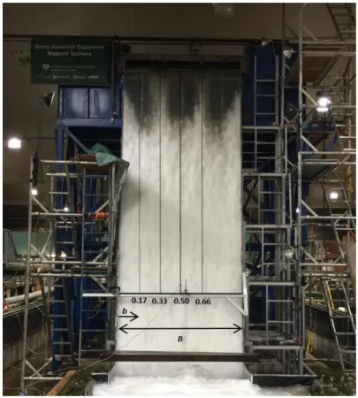
evaluated in a section of nominally equilibrium flow by measuring profiles at 19 locations across the chute, along step 23. For this set of measurements, the mounting apparatus (frame) was placed such that the probe tips were positioned over the edge of the step riser along the centerline of the chute. Then, moving the probe laterally along the axis of the frame toward either sidewall, the slight planform curvature of the chute had two effects:
1. The pseudo-bottom invert was effectively deeper along the chute centerline than near either sidewall. That difference, measured normal to the chute slope was 0.018 m relative to the sidewall pseudo-bottom invert; and
2. For lateral positions which were far from the chute centerline, (say, within the left or right pier bay), the probe tips encroached slightly beyond the edge of the numbered step, into the upstream step cavity. The maximum extent of this encroachment is shown in Figure 4.4.
The resulting data set was non-dimensionalized in the lateral axis of the chute, b/B, where b was measured from the right sidewall and B was the local chute width. The first point mentioned above was accounted for in the lateral plot of water surface by subtracting from each measured flow depth, the offset of the chute invert, which was measured at each of the 19 chute positions using the point gage with reference to the sidewall as the ‘elevation zero’.
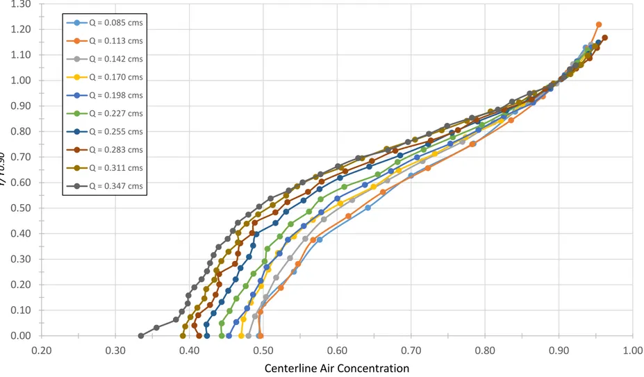
At two fixed location across step 23, near the right sidewall and along the chute centerline, profiles of air concentration were measured for 10 different discharges. The lowest discharge for this set of measurements was 0.085 m3/s. Subsequent discharges were increased in steps of 0.028 m3/s. The penultimate discharge of 0.311 m3/s was then followed by the design discharge, 0.347 m3/s.
With all recorded samples, a time-series of the air concentration could be calculated to show the fluctuations with time. Data recorded for a duration T was averaged over the full duration to determine the nominal average. Then, sub-dividing that sample into smaller durations Tw, a
moving average function showed the fluctuations with time. Calculating the standard deviation of that resulting time-series with respect to the nominal average gave a sense of the
measurements’ overall variance. Additionally, the phenomenon of roll waves was evaluated at a low discharge using the same moving average function.
Figure 3.3. The conductivity probe positioned at step 87 near the right sidewall. Step 87 corresponded with the cross-section where flow aeration had spread laterally across the entire
chute.
3.3.2
Bulk-Flow Velocity
The bulk velocity of the water mixture was determined in the same locations as the air-concentration measurements and for the same water-discharge conditions. Both values were obtained using the same conductivity probe, explained in the next section. The calculations of bulk-flow velocity were time-averaged over the sample duration, either 30 sec or 60 sec. Velocity profiles were normalized to V0.90, i.e. V(at Y=Y0.90). Values of N (i.e., the exponent of
the power function, Section 2.7) were obtained from the measured data by performing linear regressions, after log-log transformations were done.
3.4
Instrumentation
This section gives details regarding the instrumentation used to measure air concentration and bulk-flow velocity: the dual-tip conductivity probe. Along with a description of the probe’s function are details regarding the setup within the hydraulic model, the experimental methodology and an overview of the data-processing procedure.
3.4.1
Conductivity Probe
A dual-tip conductivity probe was used to measure values of air concentration within aerated regions of the chute. The probe was custom manufactured by University of Queensland. The probe operates on the premise that the electrical conductivity of water is about one-thousand times greater than that of air (Straub & Killen, 1952). Because of this, when an electrode is submerged in an air-water mixture, the resulting voltage readout fluctuated between a minimum output in air, and a maximum output in clear water.
The probe consisted of two pointed tips, offset in the flow direction by 7.0 mm. The tips were excited with electricity, and the signal of the voltage readout fluctuated as the surrounding medium transitioned between water (high electrical conductivity) and air (low conductivity). The tips were shaped as needles to facilitate the direct impingement of approaching air bubbles. Over a given sample duration, the time-averaged air concentration was obtained from the voltage time-series. First, a phase threshold was selected; i.e., a voltage value to delimit readouts in exceedance of that threshold as water, and all other readouts as air. A common threshold is taken as the average of the maximum and minimum voltage readouts (e.g., Toombes, 2002).
After a phase discrimination technique was implemented, the voltage time-series was binarized according to the voltage threshold, resulting in a time-series of the instantaneous void fraction, where C = 0 for water and C = 1 for air. The process of thresholding and binarizing was accomplished using a series of if statements in MATLAB.
The time-averaged values of air concentration were calculated as the arithmetic means of the instantaneous void fraction time-series (Chanson, 2013). The probe had a reported accuracy of 2.0% < Δ𝐶/𝐶 < 5.0%. The conductivity probe’s sampling frequency was variable and could be prescribed. For the present thesis and related hydraulic-model study, the optimum sampling