Does fuel price affect trucking industry’s network characteristics?: evidence from Denmark

Does Fuel Price Affect Trucking Industry’s Network

Characteristics? Evidence from Denmark

Megersa Abate

Swedish National Road and Transport Research Institute (VTI)

CTS Working Paper 2014:26

Abstract

The 2000s were dominated by rising fuel prices and economic recession. Both had an

impact on the structure of the trucking industry and how freight was moved. This

paper examines how fuel prices shaped trucking industry’s network characteristics

such as the average length of haul, average load, and capacity utilization. In

particular, we show the effect of fuel price on average length of haul using 29

quarterly independent surveys from the Danish heavy goods vehicle (HGV) trip diary

from 2004 to 2011. The results show that the average length of haul is sensitive to

changes in fuel price: a DKK 1 (≈0.18$) increase in diesel price/liter leads to a 4

percent decrease in the average length of haul in the 2004-2007 period. This implies

that firms improve transport efficiency by reducing the number of kilometers needed

to transport a tonne of cargo as a short run response to fuel price increases. This

result, however, is not confirmed for the years following the 2008 financial crisis. It

also depends on where in the distribution of the average length of haul one looks.

Keywords: Fuel Price; Networks; Trucking Industry; Capacity Utilization JEL Codes: Q41, R4, L92

Centre for Transport Studies SE-100 44 Stockholm

Does Fuel Price Affect Trucking Industry’s Network

Characteristics ? Evidence from Denmark

Megersa Abate∗†

December 5, 2014

Abstract

The 2000s were dominated by rising fuel prices and economic recession. Both had an impact on the structure of the trucking industry and how freight was moved. This paper examines how fuel prices shaped trucking industry’s network characteristics such as the average length of haul, average load, and capacity utilization. In particular, we show the effect of fuel price on average length of haul using 29 quarterly independent surveys from the Danish heavy goods vehicle (HGV) trip diary from 2004 to 2011. The results show that the average length of haul is sensitive to changes in fuel price: a DKK 1 (≈ 0.18$) increase in diesel price/liter leads to a 4 percent decrease in the average length of haul in the 2004-2007 period. This implies that firms improve transport efficiency by reducing the number of kilometers needed to transport a tonne of cargo as a short run response to fuel price increases. This result, however, is not confirmed for the years following the 2008 financial crisis. It also depends on where in the distribution of the average length of haul one looks.

Keywords: Fuel Price; Networks; Trucking Industry; Capacity Utilization JEL classification : Q41, R4, L92

∗_{The author would like to thank Ole Kveiborg, Bertel Schjerning and Mogens Fosgerau for helpful comments.}

Thanks also to Thomas Jensen for his help and suggestions on the data. Financial support from the Danish Strategic Research Council (through the Drivers and Limits project) and the Center for Transport Studies (KTH/VTI) are gratefully acknowledged. The usual disclaimer applies.

†_{Correspondence: Swedish National Road and Transport Research Institute (VTI), Box 8072 / SE-402 78}

1

Introduction

The sharp rise in fuel price in the 2000s reignited interest in the study of the impact of energy prices on many economic activities including transportation. Early estimates suggested that road transport costs represent about 1.6 percent of sales revenue for a typical European firm (Ross 1995). This rather small share led to the perception that much of the strategic decision-making of firms is relatively insensitive to variation in fuel prices. Although transport costs remain relatively small for shippers, fuel costs for freight carriers have always been significant because fossil fuel is still the main source of energy for motive power (Knittel 2012). The American Trucking Association estimated that the trucking industry spent nearly $115.4 billion on diesel fuel in 2011, a whopping $15 billion higher than the $101.5 billion spent on diesel in 2010 (Fender and Pierce 2012). Rising fuel price was also found to be the most important reason for energy efficiency improvement initiatives by European freight carriers (Liimatainen et al. 2012). 1 Fuel represents around 40 percent of total heavy goods vehicle (HGV) operating costs for a 44 tonne articulated truck, up from 34 percent just three years ago (The Logistics Report 2013). It is, therefore, quite reasonable to expect changes in firms’ transport behavior to changes in energy prices, especially during periods of rapid price rises.

Knowing the direction and magnitude of fuel price responses gives further ammunition for tackling the perennial question of the price sensitivity of transport activities. In freight transport, questions related to the extent of response and the mechanism of response (such as: modal shift, improvement in capacity utilization, or logistical restructuring) to changes in transport costs are still relevant. The effects of changes in the overall transport cost (cost/tonne-kilometer or cost/vehicle-kilometer) have already been well documented in the literature (see Significance and CE (2010) for a comprehensive review). The fuel price sensitivity of road freight transport, however, has been less researched. In particular, the sensitivity of the network (operating) characteristics of trucking firms such as the average length of haul, average load, and productivity (capacity utilization) to fuel price changes has been hardly touched.2

1

Firms also responded to increases in fuel prices in various ways: accumulation of inventories, centralization and modal shift (Eyefortransport, 2008).

2_{Much has been documented regarding the impact of fuel prices on consumer responses and the macro}

economy. Recent studies by Mabit (2014), Burke and Nishitateno (2013) and Clerides and Zachariadis (2010) find that higher gasoline prices induce consumers to substitute to more fuel-efficient vehicles. The impact of

This paper tackles the question of how fuel prices affect the trucking industry from two aspects. First, it estimates the direct effect of fuel price on trucking firms’ network characteristic. Specifically, it estimates the effect of changes in the price of diesel on the average length of haul and the share of loaded trips (proxies for network characteristics). The guiding hypothesis here is that during periods of high fuel prices, firms reduce the average length of hauls (the average distance a tonne of freight moves) and thereby improve the share of loaded trips of trucks. Second, a somewhat indirect effect of fuel price increase on the trucking industry is its effect on capacity utilization of trucks. To this end, the paper estimates trends in the physical productivity of trucking controlling for traffic composition.

The second line of enquiry is based on a recent study of Boyer and Burks (2009) on the productivity trends in the US trucking industry. They argue that the nominal productivity (measured in Ton-Miles per truck) of the industry increased in the period 1977-1997 as a result of shift in traffic mix towards a higher proportion of long haul movements. The deregulation of the US trucking industry and secular declines in input prices- such as fuel price and drivers compensation- were given as the underlying causes for changes in traffic composition. Boyer and Burks further argue that if the decline in input prices were to reverse, the traffic mix would also reverse back to higher proportion of short movements. This paper tests their hypothesis and analyzes the trend in traffic composition and trucking physical productivity during the high fuel prices period.

The analysis is based on a unique quarterly dataset from the Danish heavy trucks trip diary that spans 8 years. The data are disaggregated and allow for simple and flexible empirical models that control for vehicle, firm and haul characteristics. The main results confirm the above hypotheses to a reasonable degree. The price of diesel significantly affects the operating characteristics of freight movement. A DKK 1 (≈ 0.18$) increase in diesel price results in 4 to 7 percent decline in the average length of haul in the years 2004-2007. This effect disappears, however, in the years after the financial crisis of 2008. A similar pattern is observed for the effect of diesel price on the share of loaded trips vehicles make: with a significant effect in the pre-2008 period and no significant effect afterwards. As for the effect of fuel prices on traffic

oil market developments on macroeconomic outcomes is also well researched (see Carstensen et al. (2013); Kilian and Park (2009); Kilian and Lewis (2011); Kilian and Hicks (2012); Korhonen and Ledyaeva (2010). Few studies, however, look at the effect of fuel prices at an industry level. Notable exceptions are Klier and Linn (2010 and 2013) and Busse et al. (2012) who study the effect of gasoline prices on the automobile industry.

composition, confirming to Boyer and Burcks (2009) hypothesis there has been a shift towards short hauls, especially in the run up to the financial crisis of 2008 and its aftermath.

All together the findings of this paper reveal that the trucking industry is sensitive to fuel price changes and as results its traffic mix has moved towards shorter hauls. An interesting implication of these findings is that if fuel price were to continue to rise in the future, we would see more and more specialization of trucking in short haul segments where it has competitive advantage. Finally, the range of fuel price sensitiveness found in this paper could give policy makers an indication of the effect of a commensurate fuel tax increases. Taxes, understandably, have long term effects as opposed to fuel price shocks, which implies that fuel tax changes might not be similar to fuel price changes (Li et al. 2014). However, firm’s response to oil-price induced changes in fuel prices could still be an important benchmark in the trucking industry where data is rather difficult to obtain and tax increases are not politically viable. The rest of the paper is structured as follows, Section 2 reviews the literature on the relationship between fuel prices and trucking operations, Section 3 presents the econometric model and data, while Section 4 discusses the estimation results and Section 5 concludes.

2

Fuel prices and trucking operations

High fuel prices change how freight is moved by directly altering the network structure of freight carriers and by indirectly changing their traffic composition. This section presents a brief review of the literature which looks at these behavioral responses. There are three potential responses from firms (carriers/shippers) to an increase in fuel price (Significance and CE, 2010). First, they invest more in fuel-efficient vehicles or implement a more fuel efficient way of driving. Second, they improve transport efficiency or capacity utilization by reducing the number of kilometers needed to transport freight. Third, if cost increases due to fuel price rises are not fully contained through the first two mechanisms, shippers would ultimately be forced to reduce the number of tonne-kilometers.

The above responses mainly differ in terms of the time needed for implementation. Firms can adopt more fuel-efficient driving and improve transport efficiency faster than they can invest in more fuel-efficient vehicles or reduce the need for transport (as implied under the

third response).3 The adoption more fuel-efficient vehicles, however, has less than proportional effect on vehicle kilometers driven. This is because of the so called “rebound effect” which implies that improvements in fuel efficiency results in a less than proportional reduction in fuel use and hence vehicle kilometers.4

The effect of fuel price on a trucking firm can also be inferred from its effect on network characteristics such as the average length of haul (ALH) and average load or share of loaded trips (proxies for capacity utilization).5 The literature provides limited guide on how the latter variables are affected by fuel price changes. As for the ALH, however, there are many studies that relate it to a firm’s overall costs, of which fuel cost is an important part. The following paragraphs discuss possible effects of fuel price rise on the ALH and capacity utilization.

The ALH is defined as a measure of the average distance a unit of freight is moved in a single vehicle movement. It is estimated by dividing total tonne-km by total tonnes lifted (see Section 3 for a formal definition). ALH is mostly discussed in the literature in relation to the cost function. A firm’s network, which includes its ALH, is treated as an exogenous environment in which firms try to minimize (maximize) costs (profits). Such an approach is appropriate if firms operate in a regulated environment in which operating rights are determined by a regulator. It can also be justified on the basis of the very nature of freight transportation activity which depends on somewhat rigid spatial distribution of demand.6 But if firms could freely choose their network structure or if there were exogenous shocks in the economy (sharp rises in fuel price, economic recession, etc.) which change the spatial distribution of demand, the optimal network size (ALH) would be endogenously determined based on cost considerations.7

3

As pointed out by Green (1984) in terms of the production process, short-run demand for fuel is conditional upon the vehicle stock and the technology embodied in it, both of which are essentially fixed. Thus firms need to reorganize production and distribution systems, source inputs locally and invest in routing optimization technology as possible ways of reducing vehicle kilometers (McKinnon, 1999).

4_{See de Borger and Mulalic (2012) for interesting analysis of the rebound effect in trucking. Similarly,}

Kamakate and Schipper (2009) point out that improvement in the fuel economy of individual vehicles plays a small part. They discuss that large reductions in trucking energy use and emissions will come from better logistics and driving, higher load factors, and better matching of truck capacity to load. Despite being disproportional, these studies assume that the decrease in fuel use comes from reduced distance traveled.

5

Both in the literature and in industry, ALH, average load and shipment size are used as proxies for network size and density.

6_{In most cases, the locations of shippers or receivers of goods relative to major freight generators change}

only in the long run. Boyer (1993) indicates that trucking is inherently spatial in nature, and that a service from point A to point B is not a perfect substitute for a service from point C to point D; the two services are “as likely to be complements as substitutes”.

7_{Ying and Keeler (1991) treat commodity attributes or network characteristics as exogenous, but they point}

There are contradicting findings in the literature with regard to the effect of changes in ALH on trucking firm’s cost structure. One the one hand, it has been shown that firms with larger networks reduce their costs by exploiting economies of networks because larger networks allow for better utilization of specialist equipment, and afford longer hauls which are associated with more efficient use of fuel and trucks (see Friedlaender and Spady, 1980; Chiang and Friedlaender 1984; Daugherty et al., 1985). Similarly, Ying and Keeler (1991) argue that a longer ALH reduces the cost per ton-mile of a shipment because it implies lower terminal handling expense. On the other hand, Keeler (1989) and Gagne (1990) argue that if a firm has a longer ALH, for a given output level, then it will likely have a thinner route structure which implies less than optimal utilization of capacity, which will lead to higher costs.8

Evidently, the literature gives no clear guidance on how ALH affects costs or vice-versa. Would firms increase ALH to manage their operating costs? Or would they decrease it? Neither does the literature provide answers as to whether firms would increase/decrease their ALH when faced with changing economic circumstances. These are basically empirical questions, whose answers involve consideration of a firm’s vehicle choice process, inventory management, vehicle technology choice, and the relative importance of freight transport as a factor of production in the shipper’s production function. To shed light on this contradiction, Section 3 presents an econometric model which analyzes a reduced-form relationship between fuel price and the average length of haul.

A somewhat indirect effect of fuel price increase on the trucking industry is its effect on capacity utilization of trucks. If higher fuel price leads to lower average length of hauls, it is likely that this will involve some kind of improvement in capacity utilization.9 Measuring this effect is, however, rather difficult mainly due to traffic composition effects. Traffic composition effect is similar to the bias that comes from ignoring aggregation issues in productivity measures due to endogenous changes in output composition (Blundell and Stoker 2005). Because vehicles are used for transporting various items, the trucking industry is characterized

indicate that although the value and density of the commodity to be shipped are exogenous to the firm, the way in which it is shipped is not; so ALH and shipment size are endogenous to the firm, and are jointly determined with transport rate.

8_{Gagne (1990) argues that the cost elasticity of ALH depends on whether we evaluate these effects for a}

given tonne-kilometer (TKM) or a given number of shipments. If it is based on TKM, longer hauls imply lower costs, but if is based on the number of shipments longer hauls lead to higher costs.

by large heterogeneity which could lead to aggregation issues.

A recent study by Boyer and Burcks (2009) shows that the nominal productivity (measured in Ton-Miles per truck) of the US trucking industry increased in the period 1977-1997 as a result of shift in traffic composition towards a higher proportion of long haul movements.10 They cite deregulation and secular declines in input prices- such as fuel price and drivers compensation- as the main causes for changes in traffic composition. Boyer and Burks further argue that if the decline in input prices were to reverse, the traffic mix would also reverse back to higher proportion of short movements. This paper tests their hypothesis and analyzes the trend in traffic composition and trucking physical productivity during periods of high fuel prices in the Danish trucking industry.11

3

Empirical framework and data

3.1 Fuel price and average length of haul

Section 2 argued that the effect of an increase in fuel price on ALH is an open question that could only be answered with an empirical model. This Section presents an econometric model which analyzes a reduced-form relationship between the ALH and fuel price. ALH is defined by dividing total tonne-km by total tonnes lifted: ALH =P

mT KM/

P

MT where T KM

is the total tonne-kilometer for all movements (M ) of a vehicle, and T is the total tonnes lifted.Equation (1) below is a baseline regression model for the average length of haul, and Equation (3) is a model for capacity utilization.

ln ALHi,t= α + βfi,t+ γagei+ Xϕ + εi,t (1)

where the dependent variable ln ALHi,t, is the log of the average length of haul of a vehicle

i in period t; fi,t is the per-liter price of diesel; agei, is the age of a vehicle; α, β, and ϕ are

10_{Their study is based on the well-known study of the American rail roads which concluded that the}

productivity gains of railroads in the 60s was not due to the adoption of new production techniques, rather it was due to change in traffic composition (Task Force on Railroad Productivity 1973).

11_{While Danish drivers earn some of Europe’s highest wages, driver’s compensation did not increase}

dis-proportionately compared to other sectors of the Danish economy (Sternberg et al. 2014). This leaves the rapid fuel rise during the sample period as the main factor for increase in input prices for the trucking industry. If anything, in recent decades, the share of labor declined due to deregulation as in other network industries (Azmat et al. 2012).

coefficients; εi,t is a residual that is assumed to be orthogonal to the explanatory variables. β

is the parameter of interest and is expected to be negative since higher fuel expenses directly add to firms’ line-haul costs. Furthermore, a likely short run response to higher fuel prices from firms is that they will manage operating costs by cutting back haulage distances. γ is also expected to be negative as older vehicles are usually driven a lower number of kilometers.12 Furthermore, Equation (1) contains a vector of control variables, X, such as the number of axles on the vehicle, the type of firm which owns it (own-account or for-hire), and commodity and year fixed effects.

The number of axles is a proxy for vehicle carrying capacity. It is expected to affect ALH positively because firms usually employ their larger vehicles on longer hauls where there are fewer stops. As for the effect of ownership type, for-hire carriers typically have longer network as they serve several customers which are distributed over a wide geographical area. Own-account shippers, on the other hand, tend to move most of their freight from factory to factory, factory to distributor, etc which implies usage of vehicles over a limited distance range.13

Interpreting β as the impact of diesel price on ALH requires the orthogonality condition

E(εi,t|fi,t) = 0 to hold: fuel price is independent of unobserved haul, vehicle and firm

charac-teristics that do affect ALH. One potential violation of this condition arises because differences in ALH over vehicles may simply indicate differences in the unobserved spatial distribution of freight demand.14 To control for this possible source of endogeneity X includes the number of days a vehicle is used per period. This variable allows one to see the effect of fuel price conditional on the number of days used and the other control variables.

Equation (1) assumes there is no unobserved heterogeneity in impact of diesel price on ALH. However, it is possible that fuel prices affect ALH differently across vehicles of different vintage. For instance increases in diesel price could make deriving older vehicles more expensive than

12

It is important to note that older vehicles’ lower number of kilometers is partly due to the fact that they are used fewer times per period. For a given number of usages, however, older vehicles are used as much as younger ones (Hubbard, 2003). Operating cost differential affects the number of days or periods in use rather than how efficiently a truck is used per period. So, one would expect that older vehicle would be used less frequently during times of higher fuel prices.

13_{Figure 3 shows the kernel density of the distribution of ALH by firm type. It is clear from the figure that}

for-hire carriers’ vehicles are used on longer hauls

14

However, it is reasonable to expect vehicles to have a comparable distance range over which they are frequently used. Hubbard (2003) argues that most trucks are used in consistent ways from period to period.

driving younger vehicles. To test this hypothesis a more general specification is:

ln ALHi,t= α + ρfi,t× AGi+ Xϕ + εi,t (2)

Here the real diesel price, fi,t, is interacted with AGi, a dummy variable for whether the

vehicle belongs to the older vehicles category for a given period and within the same vehicle type. The age categories are: AGi= 1 if age equals 1 year or less, AGi= 2 if age equals 2 or

3 years, AGi= 3 if age equals 4 or 5 years, AGi= 4 if age equals 6 or 7 years, AGi= 5 if age

equals 8 or 9 years, and AGi= 6 if age > 9 years.

Note that identification comes from comparing the effect of diesel price on the ALH of otherwise identical vehicles that only differ in their age. The parameter ρ is identified by the time-series variation of the price of diesel and the cross-sectional variation of the age group. This identification strategy implies that firms will use their older vehicles for shorter hauls and their younger vehicles (which are probably more fuel efficient) for longer hauls. Such a strategy allows us to observe how fuel prices affect older vehicles compared with younger vehicles, not the effect of fuel price on the ALH of any given vehicle. This distinction is crucial because the latter effect cannot be distinguished from other factors that might affect both diesel price and ALH.

To check the robustness of the baseline regression, and to describe ALH differential in a more realistic fashion the baseline regression model is extended on several fronts. First, we classify the vehicles in our sample according to their Euro-class classification.15 Doing so helps one to see whether firms would prefer to use vehicles in the latest Euro-class during times of high fuel prices. Second, to fully exploit the time-dimension of the data, which is a repeated-cross-section, a cohort was defined based on vehicle type, sector and firm type. Doing so made it possible to test for the presence of inertia and whether firms were responding to contemporaneous fuel price or lagged fuel prices.

Third, many empirical applications have found quantile regression analysis useful when the variables of interest potentially have varying effects at different points in the conditional

15_{The Euro-classification is based on the classification available at the time a vehicle is observed in the sample.}

It is based on EU’s emission standards legislation which has been imposed for new vehicles sold in Europe since 1992 (Directive 2005/55/EC). The classification categories are: Pre-Euro (prior to 1992), Euro I (1992 – 30 September 1996), Euro II (1 October 1996 – 30 September 2001), Euro III (1 October 2001 – 30 September 2006), Euro IV (1 October 2006 – 30 September 2009), and Euro V (1 October 2009 onwards).

distribution of the outcome variable. While mean regression provides a valuable summary of the impact of the covariates, it does not describe the effects on different parts of the ALH distribution.16 In the context of this paper, it is likely that in the short run firms are only able to cut short hauls (e.g. feeder trips), which are less fuel efficient, implying that fuel price rises may have larger effects on short hauls than on longer hauls. To test this possibility, we use quantile regression (QR), introduced by Koenker and Bassett (1978), and analyze the effect of diesel price at several points in the distribution of ALH. All of the above regressions control commodity fixed effects to account for possible differences in the supply chain and logistical structure of moving different commodities. The regressions also contain year fixed effects to control for the average effect of the price of fuel on the ALH.

3.2 Fuel price and capacity utilization

The lower levels of ALH during episodes of high fuel prices could imply some sort of improvement in capacity utilization. This is because firms would be able to provide the same level of freight service only if they reduced empty runs or increased average load during loaded trips to improve the load factor. Relating fuel prices to vehicle utilization is, however, complicated for two reasons. First, distinguishing the pure effect of fuel price from other unobserved factors that affect capacity utilization is rather difficult because capacity utilization will change for all vehicles regardless of their age or sectors they are used in.

One way to check the relationship between fuel prices and capacity utilization is through a model that relates the share of loaded trips a vehicle makes per period and fuel price. Such a model makes it possible to see whether firms would increase the share of loaded trips if fuel prices rise so as to keep line-haul costs in check. A reduced form formulation this model is specified as:

CUi,t= τ + θfi,t+ Zϑ + ωi,t (3)

where CUi,t is the share of loaded trips in total trips (including empty runs) for a vehicle i,

in period t, a proxy for capacity utilization; Z is a vector of vehicle, haul and firm characteristics;

16_{See Wadud et al (2010) for an interesting discussion on the importance of controlling for fuel price effect}

τ , θ, and ϑ are coefficients; ωi,tis a residual that is assumed to be orthogonal to the explanatory

variables. CUi,t may not be an ideal measure of the level of capacity utilization unless we

control for the type of trips made by vehicles. As correctly pointed out by Figliozzi (2007), urban delivery vehicles usually have a higher proportion of loaded trips because it is only the last trip (usually the backhual to terminals) that is empty. On the other hand, vehicles engaged in inter-city trips face a problem of loaded backhauls that leads to a higher proportion of empty trips. To account for this operational difference, Equation 3 controls for the type of trip, distribution or normal trip.

The second reason for the complicated relationship between fuel prices and capacity utilization is the question of weather there exists a direct relationship between them (as assumed in Equation 3). It is likely that fuel prices affect trucking productivity indirectly by altering traffic composition. As argued in Section 2, high fuel prices could force carriers to shift towards shorter hauls and thereby decrease tonne-kilometers per truck. This hypothesis is tested using the method suggested by Boyer and Burcks (2009). They measure productivity at a truck level using tonne-kilometers per unit of input (the inputs being a driver and truck-tractor pulling an enclosed van).

tkmc= s X k=1 l_kctc_kmc_kw_kc (4) tkmb= s X k=1 l_kctc_kmc_kw_kb (5)

Where tkmc measures the average tonne-kilometers per truck-and-driver combination in year c; k indexes traffic segments of size s; lc_k is the proportion of trips that a truck operated loaded during year c; tc_k is the the average tonnes hauled by a vehicle in year c when it operated with a load; mc_k is the number of kilometers driven by a vehicle in year c; w_kc is the proportion of all truck traffic that is in traffic segment k in year c ; wb_k is the proportion of all truck traffic that is in traffic segment k in base year b. Each truck has three independent descriptors, distance range, sectors it is used in and commodities carried.

The effect of traffic composition is estimated by comparing the average tonne-kilometer per truck (Equation 4) with the average TKM per truck in which traffic composition is held constant at a base year (Equation 5). tkmb gives a measure of the tonne-kilometer of trucks

in a current year, under the counter factual assumption that the traffic composition had been held constant across the traffic segments as it occurred in the base year.17

3.3 Data

The main data source for the study is the Danish heavy trucks trip diary (Statistics Denmark (DST), 2011). DST has been collecting a sample of heavy trucks with a maximum legal carrying capacity of six tonnes and above since 1980. The dataset is compiled based on reports from truck owners, both for-hire carriers and own-account shippers, across Denmark. DST granted us access to the trip diary for the period 2004 to 2011.The dataset is best described as a repeated cross-section because the trip diary is filled out for different trucks in every quarter. It has detailed one-week operational information on a trip-by-trip basis for 24,106 trucks. The diaries contain information on vehicle type, number of axles, type and weight of commodity carried and haulage distance.

Diesel prices data are from the Danish Oil Industry Association (eof.dk) which has kept daily fuel prices since 1972. Much to the advantage of this research, the trip diary data contains information on the specific week in a quarter in which each truck in the sample made their trips. This made it possible to use monthly average diesel prices which resulted in an extensive variation in the diesel price variable.18

The trip diary is unique and provides disaggregated data on road freight transport which allows a detailed analysis of the trucking industry. It is the most disaggregate data on road freight transport which allows a detailed analysis unparalleled in other studies. Unlike datasets used by previous studies which are relatively aggregate (see for example Boyer and Burks, 2009; Hubbard, 2003), our dataset is very suitable to study patterns of capacity utilization and the ALH since it has a detailed (at a trip level) information for an individual truck. Although such a dataset exits in many European countries, accessing it is extremely difficult due to con[U+0085]confidentiality reasons.19 Unfortunately, Statistics Denmark changed the

17_{See Boyer and Burcks (2009) for details on how to estimate traffic composition in the context of trucking.} 18_{Diesel is the main fuel type used by heavy trucks, and it is the main fuel type used in Denmark (de Borger}

and Mulalic, 2012).

19_{Although there have been some difficulties with the collection and the representativeness of the recorded}

transports, it is still believed to be a very strong data set in relation to understanding the variation in Danish trucking. The data is also used for producing aggregate statistics in accordance with a EU directive, but there are some concerns about the precision in this regard.

commodity classification from NST/R to NTS2007 in 2008 which reduced the number of commodity types from 29 to 21. Due to the importance of this variable in the econometric analysis, the data is divided into two periods, 2004 -2007 and 2008-2011. Besides, to account for the economic recession in 2008 it would have been necessary to divide the data in a similar fashion.

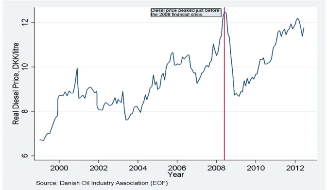
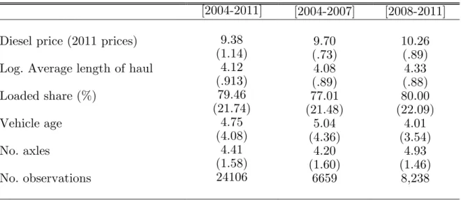
Table 1 presents summary statistics of the main variables of interest. On average, trucks appear to have higher share of loaded trips and more number of axles (which implies larger vehicles) in the 2008-2011 period. The fleet in the 2004-2007 period is, however, older and appears to have lower ALH. The low ALH in this period appears to coincide with the rapid fuel price rise shown in Figure 1. The trends of the ALH for the three vehicle types in the data are shown in Figure 2. The two heaviest vehicle types, semi-trailers and articulated trucks, have visibly longer ALH while, rigid trucks are commonly used on shorter hauls. Figure 3 displays the kernel density of ALH for own-account shippers and for-hire carriers. As shown the former have slightly lower ALH, because the latter generally tend to build extensive networks between various shippers.

4

Results

4.1 Diesel price and ALH

Table 2 reports estimates that show the relationship between the ALH and fuel price for the period 2004-2007. Each column presents results for different sets of controls, age, Euro-class, and the number of days a vehicle was operated. An increase in diesel price significantly reduces the ALH of a vehicle. The point estimates for diesel price are very similar across the models, and they show that a DKK 1 increase in price results in around 4 percent decline in the average length of hauls. As for the other explanatory variables, vehicles owned by an own-account shipper exhibit lower ALH.

As expected, larger vehicles are employed in longer hauls, whereas older vehicles are used for shorter hauls. Controlling for a vehicle’s Euro class instead of its age reveals similar patterns; vehicles belonging in the older vehicles classifications, Euro class 5 and 6, are used on shorter hauls. The last column shows that frequently used vehicles are also used to move freight over longer hauls. This is an expected result because the characteristics of a vehicle

that make a vehicle frequently used are also correlated with how far it can be used.

Table 3 reports a similar set of estimates for the period 2008-2011. Although it is statistically insignificant, the effect of diesel price appears to have been reversed in this period. This is partly due to the economic recession in the period, which might have structurally changed the pattern of freight movement. It is also challenging to find a causal effect of fuel price in this period because both fuel price and the average length of hauls might have been affected by other factors. As for the other control variables, they appear to have had comparable effects to those in Table 2.

To allow for a more flexible functional form, diesel price is interacted with indicator variables for six vehicle age groups.20 Figure 4 shows the coefficients on these interaction terms for each age group; the excluded group is age group 1, which corresponds to the youngest vehicles (Age <= 1). The negative effect of diesel price on ALH is evident as vehicles get older. However, the effects are relatively small for younger vehicles. For vehicles in groups 5 and 6, those with age > 7, a DKK 1 increase in diesel price would lead to 0.069 and 0.074 percentage point shorter haul length compared to vehicles in the first group.

One advantage of using a large sample is that it is possible to study how the effect of diesel price changes at different aggregation levels. Accordingly, the data was aggregated to form a cohort of vehicles based on three criteria: (i) the sector they are used in (agriculture, chemicals, food, mining and construction, technology, wood and paper); (ii) the type of firm which owns them (own-account shipper, for-hire carrier); and (iii) the vehicle type category they belong to (rigid truck, semi-trailers, articulated). The resulting panel data makes it possible to exploit the time dimension in the data.21 Table 4 reports a fixed effects model on the cohort data. The contemporaneous and lagged effects of diesel price are shown under columns 1 and 2, respectively. The results show that firms respond to the existing diesel price levels, not to the levels in the previous period.

All the above estimates show the effects of the explanatory variables at a single moment, that is the mean of the ALH of vehicles. Table 4 presents results from a quantile regression

20

In unreported results, the fleet size of firms was used to explore the heterogeneity of fuel price. These results, although comparable to the ones reported here, were not robust.

21_{All the variables were averaged at cohort level and estimation was done using a similar procedure to that}

that gives a richer characterization of the effect of diesel price and the control variables.22 The estimates are for quantiles: q = [0.1; 0.25; 0.5; 0.75; 0.9]. The effect of diesel price differs depending on where on the distribution of the ALH one looks. As it turns out, this effect is only significant at the 10th and 25th percentiles. This is partly due to the possibility that in the short run firms are only able to cut shorter hauls in response to higher fuel prices. Figure 5 shows the variation in the effect of the explanatory variables at the different quantiles with the 95% confidence interval. It is interesting to note that most of these effects differ in size and importance throughout the distribution of ALH.

4.2 Diesel price and capacity utilization

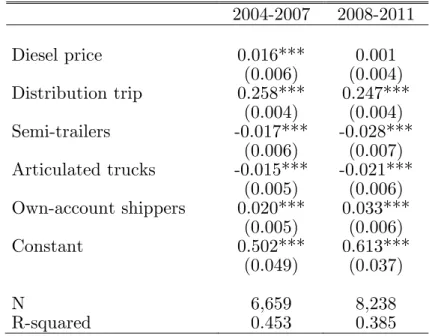
Table 6 shows the relationship between the share of loaded trips (proxy for capacity utilization) and diesel price. The results are mixed. As expected vehicles used in hauls in which there are several stops (distribution trips) appear to have higher share of loaded trips. Diesel price has a significant effect on the share loaded trips a vehicle makes in the 2004-2007 period. However, it has no significant effect in the 2008-2011 period. As indicated in Section 3 finding a causal relationship between fuel price and capacity utilization is rather difficult. This is because of the difficulty of distinguishing the pure effect of fuel price from other unobserved factors. As indicated in Section 3, another way to analyze capacity utilization in trucking is to look at trends in truck productivity.

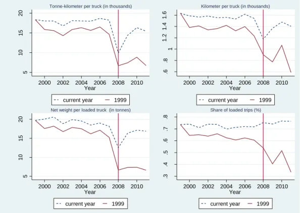
Using equations 4 and 5, a weighted average was made for truck productivity (tonne-kilometer, TKM) and its components for the entire fleet of semi-trailer trucks. Figure 6 and Figure 7 present results of these calculations. Two weighting schemes were used- one tracking the current year traffic composition and another holding traffic composition constant at the year 1999 levels. The current year TKM per truck declined at an average annual rate of 0.001% between 1999 and 2007. TKM would have declined at even higher rate of 0.03% had each of the 180 range/firm/commodity combinations had the same proportion of traffic in 2007 as it did in 1999. The rate of decline of TKM leading up-to the 2008 recession ( which simultaneously happens with the rapid fuel price rises as shown in Figure 1) is even higher.

All the components of TKM declined over the same period. Average tonne per truck saw

the largest fall by 0.01% per year. The fall is higher when traffic composition is controlled for. Had traffic composition held constant at its 1999 values, the average load would have declined over this period at even higher rate of 0.032% per year, or three times the rate. This an interesting trend especially given the trend that during this period the average carrying capacity of semi-trailer trucks increased by 0.3% per year. Boyer and Burcks (2009) give two possible answers for a similar trend observed in the US trucking industry- freight is getting less dense as the economy shifts from heavy manufacturing goods towards lighter goods, or trucks are less fully loaded. While the former resonates well with the shifts in the Danish economy, the trend in the level of the load factor on Figure 6 doesn’t really imply that trucks were getting less completely loaded. The current year weighted average load factor declined by very modest amount of only 0.003% per year.

The trend in the kilometer per truck also revels interesting shifts. During the two years leading up-to the 2008 financial crisis, the average kilometer per week driven by the average semi-trailer dropped from 1,618 to 1,177. This drop coincided with an accelerated increase in fuel price during the same period (see Figure 1). These results constitute a core evidence that during periods of high fuel prices the traffic mix moves in favor of short haul movements, as trucks are shifted from costly long haul movements confirming to predictions of Boyer and Burcks (2009) and the results in Section 3.1.

5

Conclusions

Understanding industries’ reaction to changing economic climate has always been important. This paper has examined the effect of fuel prices on the operating characteristics of the trucking industry. It proposes an empirical model which is based on the hypotheses that during periods of high fuel prices firms lower average length of hauls, the average distance a tonne of freight moves, and improve capacity utilization. The model was tested using a unique dataset from the Danish heavy goods vehicle (HGV) trip diary for 2004 to 2011. The results show that the average length of haul is sensitive to changes in fuel price with a decline ranging from 0.4 to 0.7 percent for every DKK 1 (≈ 0.18$) increase in diesel price in the period 2004-2007. This result, however, is not confirmed for the years following the 2008 financial crisis. It also depends on where I n the distribution of the average length of haul one looks. In particular,

fuel price rises are shown to have larger and significant effects only in the lower end of its distribution (10th and 25th percentiles). As for the effect of fuel price on capacity utilization, rising diesel prices led to an improvement in the number of loaded trips vehicles make per period in use. However, this effect is significant only in the period 2004-2007.

The paper has also demonstrated that physical productivity (measured in TKM) in the trucking industry had been declining during the 2000s. The run-up to the 2008 crisis saw rapid increases in fuel prices which likely triggered a shift in trucking traffic mix towards shorter-hauls. Although the load factor has remained flat, the average load and kilometers driven declined implying overall decrease in output per truck. The apparent levels of these effects are lessened, however, by changes in traffic composition. If traffic composition is controlled for, productivity differences over time in the industry appear to be even higher.

Possible caveats should be noted regarding these results. First, the fact that there is no consistent effect of diesel price on the operating characteristics for the whole sample period might imply that the findings are driven by a single episode of fuel price rises. The economic recession in the post-2008 period has also made it difficult to deduce strong causal relationships. The results should thus be interpreted with care. Second, firms’ fuel price expectations were not considered in this paper. They might, however, play an important role because of the possibility that some firms might engage in oil futures, making them less sensitive to short run price fluctuations. It was not possible to investigate this possibility in this paper due to lack of data. Third, it could be the case that the shift towards shorter hauls is prompted by fierce competition from other modes (maritime and rail) which are cheaper alternatives for long haul transport. While this might be true in geographically larger countries with well-developed infrastructure, in a small country like Denmark where trucking is still dominant the effect of other modes is less pronounced. Regardless of these caveats, the findings of this study -exploratory as they may be- represent important stepping stones for future research. They also reveal short run industry responses to energy price changes, which have not previously been studied.

An interesting question for future research is whether the shift towards shorter hauls is permanent and implies restructuring of the trucking industry’s networks. The trucking industry has long been considered to be competitive and price elastic. This in effect implied that carriers pass cost changes through to shippers without altering their network structure.

While this could still be the case, as shown in this paper the industry has restructured itself by specializing in shorter routes as a result of fuel price rises. Whether this will be a permanent feature remains to be seen conditional on the development of fuel prices and the pace of the recovery of the Danish economy. However, one implication of the findings of this paper is that if fuel price were to continue to rise in the future, we would see more and more specialization of trucking in short haul segments where it has competitive advantage. This modal share implication of fuel price rises and its effect on inventory holding of firms are worthwhile enquiries to explore in future research.

References

[1] Abate, M., 2014. Determinants of capacity utilization in road freight transport. Journal

of Transport Economics and Policy 48 (1), 137–152.

[2] Azmat, G., Manning, A., Reenen, J. V. 2012. Privatization and the Decline of Labour’s Share: International Evidence from Network Industries. Economica, 79(315), 470-492. [3] Blundell, Richard, and Thomas M. Stoker. 2005. Heterogeneity and aggregation. The

Journal of Economic Literature 43(2):347-9l.

[4] Boyer, D. K. and V. S. Burks, 2009. ‘Stuck in the slow lane: undoing traffic composition biases in the measurement of trucking productivity’, Southern Economic Journal, 75(4), 1220–37.

[5] Boyer, D.K., 1993. Deregulation of the Trucking Sector: Specialization, Concentration, Entry, and Financial Distress. Southern Economic Journal, 59(3), p.481.

[6] Burke, P. J., Nishitateno, S., 2013. Gasoline prices, gasoline consumption, and new-vehicle fuel economy: Evidence for a large sample of countries. Energy Economics, 36, 363-370. [7] Busse, M. R., Knittel, C. R., Zettelmeyer, F., 2012. Who is Exposed to Gas Prices? How Gasoline Prices Affect Automobile Manufacturers and Dealerships (No. w18610). National Bureau of Economic Research.

[8] Carstensen, K., Elstner, S., Paula, G., 2013. How much did oil market developments contribute to the 2009 recession in Germany?. The Scandinavian Journal of Economics, 115(3), 695-721.

[9] Chiang, S.J.W. & Friedlaender, A.F., 1984. Output Aggregation, Network Effects, and the Measurement of Trucking Technology. The Review of Economics and Statistics, 66(2), pp.267–276.

[10] Clerides, S., Zachariadis, T., 2008. The effect of standards and fuel prices on automobile fuel economy: an international analysis. Energy Economics, 30(5), 2657-2672.

[11] Daugherty, A., Nelson, F., and Vigdor, W., 1985. An econometric analysis of the cost and production structure of the trucking industry. In: A. Daugherty, ed. Analytical studies in transport economics. Cambridge University Press, 137.157.

[12] Deaton, A., 1985. Panel data from time series of cross-sections. Journal of Econometrics, 30(1–2), pp.109–126.

[13] De Borger, B. & Mulalic, I., 2012. The determinants of fuel use in the trucking industry— volume, fleet characteristics and the rebound effect. Transport Policy, 24(0), pp.284–295. [14] Eyefortransport, 2008. The Impact of High Fuel Prices on Logistics. Available at: http://

http://events.eft.com/fuelprices/newsstories3.shtml [Accessed December 02, 2013]. [15] Fender, K. J., Pierce, D. A. 2012. An Analysis of the Operational Costs of Trucking:

[16] Figliozzi, M.A., 2007. Analysis of the efficiency of urban commercial vehicle tours: Data col-lection, methodology, and policy implications. Transportation Research Part B: Method-ological, 41(9), pp.1014–1032.

[17] Friedlaender, A.F. & Spady, R.H., 1980. A Derived Demand Function for Freight Trans-portation. The Review of Economics and Statistics, 62(3), pp.432–441.

[18] Gagné, R., 1990. On the Relevant Elasticity Estimates for Cost Structure Analyses of the Trucking Industry. The Review of Economics and Statistics, 72(1), pp.160–164.

[19] Greene, D.L., 1984. A derived demand model of regional highway diesel fuel use.

Trans-portation Research Part B: Methodological, 18(1), pp.43–61.

[20] Hubbard, T.N., 2003. Information, Decisions, and Productivity: On-Board Computers and Capacity Utilization in Trucking. The American Economic Review, 93(4), pp.1328–1353. [21] Kamakaté, F. & Schipper, L., 2009. Trends in truck freight energy use and carbon emissions

in selected OECD countries from 1973 to 2005. Energy Policy, 37(10), pp.3743–3751. [22] Keeler, T.E., 1989. Deregulation and Scale Economies in the U.S. Trucking Industry: An

Econometric Extension of the Survivor Principle. Journal of Law & Economics, 32, p.229. [23] Kilian, L. and Park, C., 2009. The Impact of Oil Price Shocks on the US Stock Market,

International Economic Review 50, 1267–1287.

[24] Kilian, L. and Lewis, L. T., 2011. Does the Fed Respond to Oil Price Shocks?, The

Economic Journal 121 (555), 1047–1072.

[25] Kilian, L., Hicks, B., 2013. Did unexpectedly strong economic growth cause the oil price shock of 2003–2008?. Journal of Forecasting, 32(5), 385-394.

[26] Klier, T., and Linn, J., 2010. The Price of Gasoline and the Demand for Fuel Efficiency: Evidence from Monthly New Vehicles Sales Data. American Economic Journal: Economic

Policy

[27] Klier, T. and Linn, J., 2013. Fuel Prices and New Vehicle Fuel Economy—Comparing the United States and Western Europe. Journal of Environmental Economics and

Manage-ment 66: 280-300.

[28] Knittel, C.R., 2012. Reducing Petroleum Consumption from Transportation. The Journal

of Economic Perspectives, 26(1), pp.93–118.

[29] Koenker, R. & Bassett, G., 1978. Regression Quantiles. Econometrica, 46(1), p.33. [30] Korhonen, I. and Ledyaeva, S., 2010. Trade Linkages and Macroeconomic Effects of the

Price of Oil, Energy Economics 32, 848–856.

[31] Langer, A. and Miller, N.H (forthcoming). Automakers‘ Short-Run Responses to Changing Gasoline Prices. The Review of Economics and Statistics.

[32] Li, S., Linn, J. and Muehlegger, E., 2014. Gasoline Taxes and Consumer Behavior.

[33] Liimatainen, H.; Stenholm, P., Tapio, P., and McKinnon, A., 2012. Energy efficiency practices among road freight hauliers. Energy Policy, 50(0), pp.833–842.

[34] Mabit, S. L., 2014. Vehicle type choice under the influence of a tax reform and rising fuel prices. Transportation Research Part A: Policy and Practice, 64, 32-42.

[35] McKinnon, A., 1999. A logistical perspective on the fuel ef-ficiency of road freight transport. Improving Fuel Efficiency in Road Freight: The Role of Information Technologies. Available at: http://citeseerx.ist.psu.edu/viewdoc/download?doi=10.1.1.110.7044&rep=rep1&type=pdf [Accessed November 12, 2014].

[36] Ross, T., 1995. European Logistics Comparative Costs 1195. Institute of Logistics/Euro-pean Logistics Association, Corby.

[37] Significance and CE, 2010. Price sensitivity of European road freight transport towards a better understanding of existing results, Report for Transport and Environment (T&E), The Hague, Significance/CE Delft, 2010

[38] Statistics Denmark, 2011. ‘Transport of goods by road by Danish vehicles in national traffic’. Available at http://www.dst.dk/HomeUK/Guide/documentation. [Accessed 12 November 2014].

[39] Sternberg, H., Holmberg, A., Lindqvist, G., Prockl, G., 2014. Cabotagestudien: A Study on the Movement of International Vehicles in Denmark. Lunds Universitet.

[40] Task Force on Railroad Productivity (John R. Meyer, chairman), 1973. Improving railroad productivity: Final report of the task force on railroad productivity. Report to the National Commission on Productivity and the Council of Economic Advisors. Washington, D.C.

[41] Wadud, Z., Graham, D. J., Noland, R. B., 2010. Gasoline demand with heterogeneity in household responses. Energy Journal, 31(1), 47-74.

[42] Ying, J.S. & Keeler, T.E., 1991. Pricing in a Deregulated Environment: The Motor Carrier Experience. The RAND Journal of Economics, 22(2), p.264.

Table 1: Summary Statistics

[2004-2011]

[2004-2007]

[2008-2011]

Diesel price (2011 prices)

9.38

9.70

10.26

(1.14)

(.73)

(.89)

Log. Average length of haul

4.12

4.08

4.33

(.913)

(.89)

(.88)

Loaded share (%)

79.46

77.01

80.00

(21.74)

(21.48)

(22.09)

Vehicle age

4.75

5.04

4.01

(4.08)

(4.36)

(3.54)

No. axles

4.41

4.20

4.93

(1.58)

(1.60)

(1.46)

No. observations

24106

6659

8,238

Note: The cells report means, with standard deviations in parentheses. The statistics are based on Data from the Danish Heavy Vehicles Trip Diary (Statistics Denmark, 2011) and the Danish Oil Industry Association (EOF, www.eof.dk).

Table 2: Main results: Log. Average Length of Haul, 2004-2007 - Vehicle level data

[1]

[2]

[3]

Diesel price

-0.043**

-0.044**

-0.046**

(0.02)

(0.02)

(0.02)

No. axels

0.113***

0.115***

0.113***

(0.007)

(0.007)

(0.007)

Own-account carrier

-0.209***

-0.211***

-0.203***

(0.026)

(0.026)

(0.026)

Vehicle age

-0.022***

-0.020***

(0.002)

(0.003)

Euro class 3

0.047

(0.056)

Euro class 4

-0.027

(0.058)

Euro class 5

-0.158**

(0.067)

Euro class 6

-0.283***

(0.07)

Number of days used

0.032***

(0.009)

Commodity Fixed Effects

Yes

Yes

Yes

Year Fixed Effects

Yes

Yes

Yes

Constant

4.240***

4.167***

4.128***

(0.181)

(0.187)

(0.184)

N

6,659

6,659

6,659

R-squared

0.275

0.275

0.277

Note: Standard errors in parentheses. Significance is marked as: *** if p=0.01; ** if p=0.05; * p=0.1

Table 3: Main results: Log. Average Length of Haul 2008-2011 - Vehicle level data

[1]

[2]

Diesel price

0.210

0.191

(0.174)

(0.174)

No. axels

0.081***

0.083***

(0.007)

(0.007)

Own-account carrier

-0.023***

-0.288***

(0.003)

(0.028)

Vehicle age

-0.286***

(0.028)

Euro class 2

0.023

(0.026)

Euro class 3

-0.008

(0.027)

Euro class 4

-0.250***

(0.044)

Euro class 5

-0.162**

(0.079)

Euro class 6

-0.365***

(0.97)

Commodity fixed effects

Yes

Yes

Year fixed effects

Yes

Yes

Constant

3.430***

3.410***

(0.419)

(0.420)

N

8,238

8,238

R-squared

0.222

0.222

Note: Standard errors in parentheses. Significance is marked as: *** if p=0.01; ** if p=0.05; * p=0.1

Table 4: Fixed effects regressions of Log. Average Length of Haul- Cohort data

2004 - 2007

2008 - 2011

[1]

[2]

[3]

[4]

Diesel price

-0.071**

-0.071**

0.062*

0.043

(0.028)

(0.030)

(0.036)

(0.030)

Diesel price

-0.025

0.081

(0.034)

(0.052)

Vehicle age

-0.034**

-0.034*

-0.005

0.005

(0.015)

(0.017)

(0.022)

(0.016)

Chemicals

-0.038

-0.055

0.003

-0.005

(0.064)

(0.068)

(0.106)

(0.105)

Food

0.115*

0.114*

0.122

0.104

(0.057)

(0.058)

(0.084)

(0.083)

Mining and construction

-0.410***

-0.418***

-0.459***

-0.476***

(0.067)

(0.069)

(0.114)

(0.107)

Technology

0.142***

0.142***

-0.023

-0.063

(0.050)

(0.051)

(0.082)

(0.084)

Semi-trailers

0.260***

0.259***

0.269***

0.228***

(0.049)

(0.050)

(0.078)

(0.070)

Articulated

0.349***

0.340***

0.469***

0.422***

(0.052)

(0.058)

(0.082)

(0.068)

Own-account

-0.104**

-0.113**

-0.220***

-0.257***

(0.045)

(0.047)

(0.071)

(0.074)

Wood and paper

-0.172

-0.212**

(0.121)

(0.098)

Year fixed effects

Yes

Yes

Yes

No

Year_2008

-0.246**

-0.244***

Constant

5.123***

5.193***

3.768***

3.182***

(0.332)

(0.314)

(0.414)

(0.689)

Observations

464

452

439

392

R-squared

0.434

0.437

0.317

0.394

Note: Standard errors in parentheses. Significance is marked as: *** if p=0.01; ** if p=0.05; * p=0.1

Table 5: Quantile Regressions of Log. Average Length of Haul, 2004-2007

q=.10 q=.25 q=.50 q=.75 q=.90

Disel price

-0.092**

-0.065*

-0.022

-0.017

-0.009

(0.040)

(0.033)

(0.026)

(0.026)

(0.021)

No. axles

0.139*** 0.141*** 0.123*** 0.088*** 0.082***

(0.005)

(0.004)

(0.003)

(0.004)

(0.003)

Own-account carrier

-0.301*** -0.233*** -0.203*** -0.170*** -0.135***

(0.010)

(0.010)

(0.007)

(0.007)

(0.009)

Vehicle age

-0.027*** -0.021*** -0.018*** -0.020*** -0.016***

(0.040)

(0.034)

(0.040)

(0.029)

(0.033)

Constant

3.666*** 3.893*** 3.930*** 4.628*** 4.913***

(0.372)

(0.279)

(0.219)

(0.232)

(0.182)

Pseudo R

_0.16

_0.18

_0.17

_0.15

_0.12

Observations

6,659

6,659

6,659

6,659

6,659

Note: Standard errors in parentheses. Significance is marked as: *** if p=0.01; ** if p=0.05; * p=0.1. Standard errors were calculated through 299 bootstrap replications.

Table 6: Capacity utilization and diesel price

2004-2007 2008-2011

Diesel price

0.016***

0.001

(0.006)

(0.004)

Distribution trip

0.258***

0.247***

(0.004)

(0.004)

Semi-trailers

-0.017***

-0.028***

(0.006)

(0.007)

Articulated trucks

-0.015***

-0.021***

(0.005)

(0.006)

Own-account shippers

0.020***

0.033***

(0.005)

(0.006)

Constant

0.502***

0.613***

(0.049)

(0.037)

N

6,659

8,238

R-squared

0.453

0.385

Note: The dependent variable is the share of loaded trips. Standard errors in parentheses. Significance is marked as: *** if p=0.01; ** if p=0.05; * p=0.1

Figure 1: Inflation-adjusted price of diesel

Note: The diesel prices are monthly averages in 2010 prices.

Figure 2: Average Length of Haul by vehicle type

Note: The solid horizontal line indicates the mean of average length of haul (87 km) during the sample period.

Figure 3: Kernel density estimates by firm type

Figure 4: Effect of diesel price on average length of haul (ALH) by age group

Note: This figure shows the effect of diesel price on average length of haul by age group. The effects are relative to the youngest age group 1

, which corresponds to the youngest vehicles

(Age <= 1).

Figure 5: Quantile regression and OLS coefficients

Note: This figure displays quantile regression and OLS coefficients with 95-percent confidence intervals for each explanatory variable for quantiles: q = [0.1; 0.25; 0.5; 0.75; 0.9]. For most of the

1

The commodity (com) classification is: com=1, live animals (reference group); com=2, cereals; com=3 Vegetables, fruits and flower; com = 4, Sugar beets; com=5, wood; com=6, skin and leather; com=7, Food; com=8, fodder and straw ; com=9, fat from animals and plants; com=10, coal; com=11, crude oil; com=12, gasoline and other petroleum; com=13, iron ore and iron waste; com=14, ores and waste of other metals; com=15, semi-manufactured articles; com=16, gravel, soil, stone and salt; com=17,cement, chalk and bricks; com=18, fertilizers; com=19, tar and asphalt; com=20, chemical products; com=21, cellulose, paper waste etc; com=22, machinery and vehicles (including parts).

variables, the marginal effect varies with q. The OLS coefficients (denoted by horizontal broken line), however, are constant.

Table 6: Trends in Tonne-Kilometer per truck and its components with current year and

constant (1999) traffic proportions

5 10 15 20 2000 2002 2004 2006 2008 2010 Year current year 1999

Tonne-kilometer per truck (in thousands)

.6 .8 1 1 .2 1 .4 1 .6 2000 2002 2004 2006 2008 2010 Year current year 1999

Kilometer per truck (in thousands)

5 10 15 20 2000 2002 2004 2006 2008 2010 Year current year 1999

Net weight per loaded truck (in tonnes)

.3 .4 .5 .6 .7 .8 2000 2002 2004 2006 2008 2010 Year current year 1999

Table 7: Annual changes in Tonne-Kilometer per truck and its components with current

year and constant (1999) traffic proportions

-1 -. 5 0 .5 2000 2002 2004 2006 2008 2010 Year current year 1999

Tonne-kilometer per truck

-. 6 -. 4 -. 2 0 .2 .4 2000 2002 2004 2006 2008 2010 Year current year 1999

kilometer per truck

-. 8 -. 6 -. 4 -. 2 0 .2 2000 2002 2004 2006 2008 2010 Year current year 1999 weight in tonnes -. 4 -. 2 0 .2 2000 2002 2004 2006 2008 2010 Year current year 1999 load factor