MASTER THESIS IN MATHEMATICS /APPLIED MATHEMATICS
Java Applet for the Pricing of Exotic Options by Monte-Carlo
Simulations in a Lèvy market with Stochastic Volatility
by
Isaac Acheampong
Magisterarbete i matematik / tillämpad matematik
DEPARTMENT OF MATHEMATICS AND PHYSICS
MÄLARDALEN UNIVERSITY
SE-721 23 VÄSTERÅS, SWEDEN
DEPARTEMENT OF MATHEMATICS AND PHYSICS
___________________________________________________________________________
Master thesis in mathematics / applied mathematics
Date:
2006-02-24
Projectname:
Java Applet for the Pricing of Exotic Options by Monte-carlo simulations in a Lèvy market
with Stochastic Volatility
Author:
Isaac Acheampong
Supervisor:
Dr. Anatoliy Malyarenko
Examiner:
Prof. Dmitrii Silvestrov
Comprising:
10 points
___________________________________________________________________________
“We must accept finite disappointment, but we must never lose infinite hope”.
--Dr. Martin Luther King Jr
by Isaac Acheampong Mälardalen University
1
Acknowledgement
Lots of thanks to God for his blessing with life. My thanks go to my supervisor Dr. Anatoliy
Malyarenko for his guidance and advise in this thesis, Dr Wim Shoutens for his suggestions
and advice I also thank Dr Henrik Jönsson and all lecturers and professors in the Analytical
Finance programme for their inspiration and patience whiles training me in this interesting
field. Lot of thanks to my wife Pernilla and my family for their support. To all my friends and
colleagues I say thanks.
by Isaac Acheampong Mälardalen University
2
Abstract
Most financial models including the famous Black & Scholes model assumes constant
volatility. However in recent times modellers at major financial institutions are modelling
stock prices based on stochastic volatility models. One such way is when stock prices are
assumed to undergo Lévy processes with stochastic volatility.
Based on this, exotic options like the barrier and look back options are priced using
Monte-Carlo simulations. The sampling of the processes is based on time changed technique of the
Lévy processes involved. A Java applet is developed to price this options and to calculate the
standard errors.
by Isaac Acheampong Mälardalen University
3
Executive summary
In the last couple of years, the size of world’s exotic options market has grown considerably.
Today a large diversity of such instruments is accessible to investors and they can be used for
numerous purposes. Numerous factors can provide a clarification for the recent success of
these instruments. One likelihood is their almost boundless flexibility in the sense that they
can be personalized to meet the precise needs of any investor. Hence them being sometimes
referred to as customer-tailored options or special-purpose options.
These options also play an important hedging role and, thus, they meet the hedgers’ needs in
gainful ways. Corporations have left buying some form of general protection to designing
strategies to meet precise exposures to risk at a given point in time. These strategies can be
based on exotic options which are less expensive and much more efficient than standard
instruments. Many exotic options have been priced either numerically or analytically.
The approach we adopt for pricing is based on Monte Carlo simulations and it is
implemented in Java.
by Isaac Acheampong Mälardalen University
4
Table of Content
1.0 Inroduction……….……….…..6
2.0 Derivatives pricing………..……….….9
2.1 Vanilla Options……….9
2.2 Exotic Options……….……10
2.2.1 Barrier and Lookback options………10
2.2.1.1
Down-Out-Barrier
Options………..…...10
2.2.1.2
Down-In-Barrier
Options……….10
2.2.1.3
Up-In-Barrier
Options………...11
2.2.1.4
Up-Out-Barrier
Options………..11-12
3.0 Lévy Processes……….13-14
3.1 Examples of Lévy processes………....15
3.1.1 Normal Inverse Guassian Processes………....15
3.1.2 Variance gamma processes……….…15-16
4.0 Lévy Stochastic Volatility Modelling……….…...16-17
5.0 Monte Carlo Simulation Of Stochastic Volatility Lévy Processes………...18-20
6.0 The LSVP Jave Applet………21
6.1 The Concept………..21
6.2 The Structure and Recommendation on How to Run………..21
6.3 User manual………..22
6.3.1 Start of the Program……….22
6.3.2 Overview of LSVP’s User interface……….22
6.3.3 Description of Components………...………...23
6.3.3.1
Graphics
panel………...23
6.3.3.2
Process
Panel………..23
6.3.3.3
Simulations
Panel………...24
6.3.3.4
Action
Pane………...25
6.3.3.5 Option Type panel………25-26
6.3.3.6
Parameter
panel……….26
6.3.3.7
Output
Panel………...27
6.2 Some Pricing Results…...27-32
7.0 Conclusion……….33
8.0 References……….34-35
9.0 Appendix………..36-94
by Isaac Acheampong Mälardalen University
5
Introduction
The revolution of financial instruments pricing was escalated with the introduction of the
famous continuous time Black-Scholes model. It prices stocks or indices with the assumption
that their returns undergo log normal distribution. The price process of the underlying is given
by the geometric Brownian motion
,
2
exp
2 0⎟⎟
⎠
⎞
⎜⎜
⎝
⎛
+
⎟⎟
⎠
⎞
⎜⎜
⎝
⎛
−
=
t tS
t
W
S
μ
σ
σ
where
{
is a standard Brownian motion .With this formula various options can be
developed, mainly the plain vanilla options and the exotic options , one of particular interest
for this thesis is the pricing of the exotic options(so called path dependent options) of
European nature.
}
0
,
t
≥
W
tThe plain vanilla products have standard well-defined properties and trade actively. Their
prices or implied volatilities are quoted by exchanges or by brokers on a regular basis. One of
the exciting aspects of over-the-counter derivatives market is the number of non-standard (or
exotic) products that have been created by financial engineers. Even though the usually make
up a very small percentage of a portfolio they are usually much more profitable than the plain
vanilla products. Exotic options are created for a number of reasons. Sometimes they meet a
genuine hedging need in the market; there could be tax, accounting, legal or regulatory
reasons why corporate treasurers find exotic option attractive. They could also be designed
to reflect a corporate treasurers perceptions about the future movement of a market variable.
However because of its flexible nature they can be made to seem more attractive than it is for
an unwary corporate treasurer.
In this paper interest is focused on the so called barrier options and the lookback options to
investigate the pricing procedures. Since there exist traditional pricing procedures a method
by way of the principles of Lévy processes is adopted. It is also investigated into detailed the
idea of stochastic volatility which is incorporated, this is a drawback in the Black-Scholes
model which assumes a constant volatility. Hence for any pricing the value is dependent
heavily on the choice of the constant volatility estimate. The relaxation of these strong
assumption in the Black-Schole world makes modelling much more realistic.
Analytical formulas are available in the BS-world however numerical procedures need
incoporated if the Lévy stochastic volatility modelling is to be used. Path-dependent options
by Isaac Acheampong Mälardalen University
6
are now very popular in the OTC market in these last decades. Examples of exotic type
path-dependent options are lookback options and barrier options. The lookback option gives its
holder the right but not the obligation to buy (call type lookback) or sell (put type look back)
the stock at the minimum or maximum respectively it has attained over the life of the option.
The value of barrier option depends on whether the price of the underlying asset crosses a
given threshold (the barrier) before maturity. The simplest barrier options are “knock in”
options which become alive when the price of the underlying asset touches the barrier and
“knock-out” options which goes out of existence (become dead) in the case. E.g. an
up-and-out call or put has the same payoff as a regular plain vanilla call or put whiles the price of the
underlying assets stays below the barrier during the life of the option but becomes valueless
as soon as the price of the underlying asset crosses the barrier. The Black-Scholes framework
gives a closed-form option pricing formulae for the above types of barrier and lookback
options ([2]). It has been established that the log-returns of most financial assets are
asymmetrically distributed and have an actual kurtosis that is higher than that of the Normal
distribution. The Black-Scholes model is thus a very poor model for describing stock price
dynamics. In real life traders aware that the future probability distribution of an underlying
asset may not always be log normal hence they use a volatility smile adjustment. The
volatility smile-effect is diminishing with time to maturity. To price a set of European vanilla
options, one uses for every strike K and for each maturity T a chosen volatility parameter
which is basically wrong since this implies that only one underlying stock/index is modeled
by a number of utterly different stochastic processes. What is more,one cannot guarantee that
the choice of volatility parameters can be used to price exotic options.
To handle the non-Gaussian nature of the log-returns, in the last two decades
several other models, based on more complicated distributions, were proposed. In these
models the stock price process where considered to be an exponential of a so-called Lèvy
process. As for a Brownian motion, the Lèvy process has stationary and independent
increments; however the distribution of the increments must now belong to the class of
infinitely divisible laws. Choosing this law is crucial in the modeling and it should reflect the
stochastic behavior of the log-returns of the asset.
In [3] (Madan and Seneta) and in [4] (Barndorff-Nielsen) proposed a Lèvy process with
Variance Gamma and Normal Inverse Gaussian (NIG) distributions respectively. These
models are better at calibration of model prices to market prices than the BS-models, even
though this will not be investigated in this paper it is worth mentioning. The models are better
by Isaac Acheampong Mälardalen University
7
fit to historical data as well. Even with a significant improvement in accuracy with respect to
the BS-model by financial modelers, there is still is a discrepancy between model prices and
market prices. In using these Lèvy models one need to note the main feature which these
models are missing, i.e. the fact that the volatility or more general the environment is varying
stochastically over time. Stochastic volatility is a stylized feature of financial time series of
log-returns of asset prices.
To deal with this problem, one begins with the Black-Scholes setting and makes the
volatility parameter itself stochastic. A variety of choices can be made to describe the
stochastic behavior of the volatility. The Cox-Ingersoll-Ross (CIR) square root process was
mentioned and used in this case as proposed in [6].
The focus was on the introduction of the stochastic situation through the stochastic time
change as proposed in [6]. This technique is not necessarily used starting from the BS-model,
but could be used with Lèvy models as well. In these stochastic volatility models the business
time (of the Lèvy process) is made stochastic, i.e. in periods with high volatility time is
running fast, and in periods with low volatility the time is running slow. For this rate of time
process, leads to the choice of the proposal in [6] a classical example of a mean-reverting
positive process: the CIR process. Based on these models and the idea of Monte-Carlo
simulations a Java applet was developed to price barrier and look back options. Finding
explicit formulae for exotic options is very difficult if not impossible in these models.
However, once the model is calibrated to a basic set of options, it is easy to price other
(exotic) options using Monte-Carlo simulations. With the choice of the time-changing process
(ie.in my case CIR) the complexity of the simulation is not made any more difficult than the
Lèvy process.
In section 5.0 I performed a number of simulations to compute option prices for
both the VG and NIG models. I also did simulations to compute the standard error of the
models option prices. It is shown in [1] that the standard error of the simulations can be
reduced if the technique of control variates is used however this was not investigated in this
paper.
Derivatives pricing
All the way through the text I denote the daily interest rate with r and the dividend yield per
year with q unless otherwise stated. Assumption of a fixed forecasting horizon T and a market
by Isaac Acheampong Mälardalen University
8
with a single riskless asset (one bond) with a price process given by
B
=
{
B
t=
e
rt,
0
≤
t
≤
T
}
and one risky asset (the stock) with price process
S
=
{
S
t,
0
≤
t
≤
T
}
.
Focus is on the
European-type derivatives, hence no exercise prior to expiration is possible. For the market model, let
represent the payoff of the derivative at its time of expiry T.
{(
S
u
T
G
u,
0
≤
≤
})
]
According to the fundamental theorem of asset pricing [15] the arbitrage free price of
the derivative at time
t
P
[
T
t
∈
0
,
is given by
Q[
r(T t)(
{
u,
0
}
)
t]
,
tE
e
G
S
u
T
f
P
=
− −≤
≤
where the
expectation is taken with respect to an equivalent martingale measure Q and
is the natural filtration of the price process
{
f
t
T
f
=
t,
0
≤
≤
}
S
=
{
S
t,
0
≤
t
≤
T
}
.
An
equivalent martingale measure is a probability measure which is equivalent (.i.e. has the same
null-sets) to the given (historical) probability measure and under which the discounted process
( )
{
t}
t T rS
e
− −is a martingale. Models with only one equivalent measures are said to be complete
and those with more than one equivalent measures are said to be incomplete.
Vanilla options
Carr and Madan [11] were the first to develop a general pricing method, which is applicable
when the characteristic function of a risk-neutral stock price process is known. In [11] it was
shown that the price of an European call option C(K,T) with strike K expiration T and
α
being a positive constant such that the
α moment of the stock price exist is given by
th
(
)
(
( )
)
∫
+∞(
( )
) (
−
−
=
0exp
log
log
exp
,
T
K
iv
K
v
dv
K
C
ψ
π
)
α
,
where α is a positive constnt ,and the characteristic function
( )
[
(
(
(
(
)
) ( )
)
)
]
v
i
v
S
i
v
i
E
e
v
T rT1
2
log
1
exp
2 2+
−
+
+
+
−
=
−α
α
α
α
ψ
The price of an the corresponding put option can be found using the put-call parity.
Exotic options
Barrier and Lookback options
To explain the valuation of the lookback and barrier options, first consider an option contract
that expires at time T, and has a maximum and minimum process respectively. If the process
is
Y
=
{
Y
t,
0
≤
t
≤
T
}
, then let the maximum process be;
M
{
Y
uu
t
}
,
Yt
=
sup
;
0
≤
≤
by Isaac Acheampong Mälardalen University
9
and the minimum process being
m
inf
{
Y
u;
0
u
t
}
,
Yt
=
≤
≤
0
≤
t
≤
T
. Then using the
risk-neutral pricing, the price of a lookback call option is given by
⎥
,
⎦
⎤
⎢
⎣
⎡
−
=
− s T T Q rTm
S
E
e
LC
and that of a lookback put option is given by
⎥
.
⎦
⎤
⎢
⎣
⎡
−
=
− T S T Q rTS
M
E
e
LP
For barrier options, specifically the single barrier type options, the following are considered.
Down-and-out barrier option:
This type of barrier option is worthless except if its minimum remains above some level H.
Usually this level H is initially set below the initial value of the underlying (stock). If it
remains above the barrier H until maturity then it retains the structure of an European call or
put with strike K.The initial price at t =0 is
(
)
(
)
⎥
⎦
⎤
⎢
⎣
⎡
>
−
=
− +H
m
K
S
E
e
DOB
call rT Q T1
TSand
(
)
(
)
⎥
⎦
⎤
⎢
⎣
⎡
>
−
=
− +H
m
S
K
E
e
DOB
put rT Q T1
TSfor a Call and Put ,respectively.
Down-and-in barrier option:
This type of barrier option is worthless except if its minimum went below some level H.
Usually this level H is initially set below the initial value of the underlying asset (stock). If it
remains above the barrier H until maturity then it is worthless. However if its minimum goes
below the barrier H then it retains the structure of an European call or put with initial price i.e.
at t =0, given by;
(
)
(
⎥
⎦
⎤
⎢
⎣
⎡
≤
−
=
− +H
m
K
S
E
e
DIB
T TS Q rTcall
1
)
for a call contract and
by Isaac Acheampong Mälardalen University
10
by Isaac Acheampong Mälardalen University
11
)
)
)
)
)
(
)
(
⎥
⎦
⎤
⎢
⎣
⎡
≤
−
=
− +H
m
S
K
E
e
DIB
put rT Q T1
TSfor a put contract
Up-and-in barrier option:
This type of barrier option is worthless except if its maximum goes above some level H.
Usually this level H is initially set above the initial value of the underlying (stock). If this
barrier is crossed during the life of the contract; it retains the structure of an European call or
put with strike K. The initial price is therefore given by
(
)
(
⎥
⎦
⎤
⎢
⎣
⎡
≥
−
=
− +H
M
K
S
E
e
UIB
T TS Q rTcall
1
for a call contract and
(
)
(
⎥
⎦
⎤
⎢
⎣
⎡
≥
−
=
− +H
M
S
K
E
e
UIB
put rT Q T1
TSfor a put contract.
Up-and-out barrier option
This type of barrier option is worthless except if its maximum remains below some level H.
Usually this level H is initially set above the initial value of the underlying (stock). If this
barrier is never crossed during the life of the contract, then it retains the structure of an
European call or put with strike K. The initial price, t =0, is therefore given by
(
)
(
⎥
⎦
⎤
⎢
⎣
⎡
<
−
=
− +H
M
K
S
E
e
UOB
T TS Q rTcall
1
for a call contract and
(
)
(
⎥
⎦
⎤
⎢
⎣
⎡
<
−
=
− +H
M
S
K
E
e
UOB
put rT Q T1
TSfor a put contract .
It can be easily observed that a vanilla option with strike K can be constructed from either a
combination of a DIB and DOB options with barrier H and strike K.Likewise a combination
of UIB and UOB with same strike K and barrier H will give a corresponding vanilla with
strike K. Letting C and P denote call and Put price respectively, then
(
)
(
)
(
(
) (
)
)
⎥
⎦
⎤
⎢
⎣
⎡
>
+
≤
−
−
=
+
+H
m
H
m
K
S
E
rT
DOB
DIB
call callexp
Q T1
TS1
TS(
)
(
)
);
,
(
exp
T
K
C
K
S
E
rT
Q T=
⎥⎦
⎤
⎢⎣
⎡
−
−
=
+(
)
(
)
(
(
) (
)
)
⎥
⎦
⎤
⎢
⎣
⎡
>
+
≤
−
−
=
+
+H
m
H
m
S
K
E
rT
DOB
DIB
TS S T T Q put putexp
1
1
(
)
(
)
);
,
(
exp
T
K
P
S
K
E
rT
T Q=
⎥⎦
⎤
⎢⎣
⎡
−
−
=
+For the up and in barrier options the illustration is as follows;
(
)
(
)
(
(
) (
)
)
⎥
⎦
⎤
⎢
⎣
⎡
<
+
≥
−
−
=
+
+H
M
H
m
K
S
E
rT
UOB
UIB
call callexp
Q T1
TS1
TS(
)
(
)
);
,
(
exp
T
K
C
K
S
E
rT
Q T=
⎥⎦
⎤
⎢⎣
⎡
−
−
=
+(
)
(
)
(
(
) (
)
)
⎥
⎦
⎤
⎢
⎣
⎡
<
+
≥
−
−
=
+
+H
M
H
m
S
K
E
rT
UOB
UIB
TS S T T Q put putexp
1
1
(
)
(
)
);
,
(
exp
T
K
P
S
K
E
rT
T Q=
⎥⎦
⎤
⎢⎣
⎡
−
−
=
+Hence it can be concluded that the price of a plain vanilla option is related with that of a
corresponding barrier option. The price process of the underlying are in practice usually
observed at a close of a trading day to check if a barrier has been crossed, for the above
formulation however, observations are assumed to be on a continuous basis. [7] and [8]
proposes a ways of adjusting the Black-Scholes setting for the case of discrete observations
for a lookback options and barrier options respectively. For barrier H is replaced with
⎟
⎠
⎞
⎜
⎝
⎛
m
T
H
exp
0
.
582
σ
for an up-and-in or up-and-out and
⎟
⎠
⎞
⎜
⎝
⎛−
m
T
H
exp
0
.
582
σ
for the
DIB and DOB options.where m is the number of observations and
m
T
is the time between
by Isaac Acheampong Mälardalen University
12
observations.In this paper a year is assumed to be 250 days and observations are assumed to
be made at the end of a trading day.
Lévy processes
Any real valued stochastic process (
X
t∈ ,[0∞)) on a filtered probability space
(
Ω
,
F
t∈[0,∞),P
)
is
said to be a Lévy process if
(a) It starts at zero i.e for a stochastic process
X
=
{
X
t,
t
≥
0
}
,
X
0=
0
,
with
.
(
X
0=
0
)
=
1
P
(b) Its increments are independent, i.e. for
0
≤
s
<
s
1<
s
2....
<
s
n<
∞
, and
... are independent random variables
,
1 S SX
X
−
1 2 S SX
X
−
(c) Has stationary increments (ie.time homogenous ) i.e for
as the
same distibutions as
. It therefore means the distributions of increments does not
depend on t but depends on the distance between two time moments.
t h t
X
X
t
≥
0
,
+−
h
hX
(d) It is a continuous stochastic process i.e.
∀
ε
>
0
,
lim
(
)
0
0 +
−
≥
=
→ t h t
ε
h
P
X
X
.
(e) Its sample path (trajectories ) is right continuos with left limit almost surely,i.e,
∀
t
∈
[
0 T
,
)
,
+
,
> →ts t s=
t slim
,X
X
− < →ts t s
=
t slim
,X
X
and
X
t+=
X
t,
As you can see, the fact that left continuity is not needed allows the process to have
jumps.It can be proved that
X
thas an infinitely divisible distibution for
∀
t
∈
[
0 T
,
)
,
.
Let
X
be a random variable with its probability density function
P
. From[16] a
characteristic function
φ
x( )
w
with ω∈R is defined as the Fourier transform of the probability
density function
P
( )
[
( )
]
∫
∞[ ]
∞ −≡
Ρ
≡
Ρ
≡
iwx iwx xw
f
x
e
(
x
)
dx
E
e
φ
by Isaac Acheampong Mälardalen University
13
From [16], a real valued random variable
X
with a probability density function P(x)
and a
characteristic function
φ
x( )
w
is said to be infinitely divisible if for
∀
t
∈
[
0 T
,
)
,
there exist i.i.d
random variables
X
1,
X
2,....,
X
nwith a characteristic function
φ
Xi(w
)
such that:
(
n X X(
w
)
φ
i(
w
)
φ
=
)
……….(1)
or
)
(
))
(
(
1/w
w
i X n Xφ
φ
=
P
is said to be an infinitely divisible distribution.
In [16] it is proposed and proved that, If
is a real valued Lévy process on a filtered
probability space
[ ∞) ∈ ,0 tX
[ )(
Ω
,
F
t∈0,∞,P
)
, then
X
thas an infinitely divisible distribution for
∀
t
∈
[
0
,
T
)
.
Where
Φ
(
w;
X
t)
is the characteristics function of
X
tand
Φ
(
w
;
X
ti−ti−1)
be the
characteristic function of the i.i.d increments.It is obvious from the property of characteristic
functions(ie.for independent random variables the characteristic function of their sum is equal
to the product of their characteristic functions).
Hence if
{
X
k,
k
=
1
,
2
,..
n
}
then
∏
==
n k k X X X nw
w
1 ,... , 2(
)
(
)
1φ
φ
,
making equation (1) hold for such a characteristic function
φ
X(w
)
given for
∀
w
ε
R
,
))
(
exp(
)
(
w
Xw
Xψ
φ
=
.
where
ψ
X(w
)
is a log Characteristics function given by [1] as;
{
}
{
exp(
)
1
1
}
(
)...
...
...
...
...(
2
)
2
)
(
w
Aw
2i
w
iwx
iwx
x 1L
dx
X∫
∞ ∞ − ≤−
−
+
+
−
=
γ
ψ
where A= unique non-negative constant called the Gaussian variance (
.
σ
2)
ie
γ
is a real constant
L is a measure on R satisfying
{ }
{ }
( )
<
∞
=
∫
∞ ∞ −dx
L
x
and
L
1
,
.
min
,
0
)
0
(
2which is a Lévy measure .
by Isaac Acheampong Mälardalen University
14
From (2), it can be seen that Lévy processes consist of three parts: linear deterministic
parts(drift) i.e (i
γ
w),brownian part (.ie.
2
2
Aw
−
) and the pure jump part. This triplets are
written as (
γ
,A,L(dx)).The Lévy measure dictates how the jumps occur. For A=0,
{ }
<
∞
∫
∞ ∞ −Ldx
x 1
2,
, then from the theory of standard Lévy processes, the process has finite
variation. However for A=0,
∫
∞{ }
=
∞
∞ −
Ldx
x 1
2,
, and the process has infinite variation.
Examples of Lévy processes
The Normal Inverse Gaussian process:
The Normal inverse Gaussian (NIG) distrubution was introduced initially by
Barndorff-Nielsen[9] and later work was done by other researchers such as Rydberg ,T(1996)[10]
The density of NIG(
α
,
β
,
δ
) distribution is given as
2 2 2 2 1 2 2
)
(
)
exp(
)
,
,
:
(
x
x
K
x
x
f
NIG+
+
+
−
=
δ
δ
α
β
β
α
δ
π
αδ
δ
β
α
From [9] it is known that the characteristic function of the NIG distribution with parameters
,
,
0
α
β
α
α
<
−
<
<
and
δ
>
0
,is given by
))
)
(
(
exp(
)
,
,
;
(
α
β
δ
δ
α
2β
2α
2β
2φ
NIGu
=
−
−
+
iu
−
−
,
clearly it is an infinitely divisible characteristic function.Its Lévy measure is given by [1]
as
dx
x
x
K
x
dx
L
NIG(
)
exp(
β
)
1(
)
π
δα
=
,
Its Lévy triplet is given as [
γ
NIG,
0
,
L
NIG(
dx
)
] where
=
∫
1 0 1
(
)
)
sinh(
)
2
(
x
K
x
dx
NIGπ
β
α
δα
γ
and
K
1( )
x
denotes the modified Bessel function of the third kind with index 1(see[14]).
The Variance Gamma process:
The variance gamma (VG) process is defined by evaluating a Brownian motion with drift
θ and volatility σ at a gamma time.
)
(
)
,
,
;
(
L t L t VGt
L
G
W
G
X
σ
θ
=
θ
+
σ
where
L tG = gamma process with mean rate t and variance rate rt
by Isaac Acheampong Mälardalen University
15
The probability density function of the VG-distrubuted random variable G at time t is
)
(
)
/
(
)
(
/ / 1L
t
L
e
L
t
G
G
f
L t L GΓ
=
− −where L is the Lévy measure
The Characteristic function of the VG process is evaluated as
[
iuX t]
t L VGu
L
L
iu
e
E
t
t
L
t
u
VG / 2 2 ) ()
2
1
(
)
,
,
;
(
σ
θ
=
=
−
θ
+
σ
−φ
This distribution is infinitely divisible and defined as the VG-process
=
{
( ),
≥
0
}
,
t
X
X
VG tVGwhich is a process which starts at zero, has independent and stationary increments and where
the increments
VG, over the time interval [s,s+t] follows a VG(
s VG t s
X
X
+−
σ
t
θ
t
L ,
,
) law. In [5]
it was shown by Carr, Chang and Madan that the variance gamma process may also be
expressed as the difference of two independent gamma process with one describing the up
move and one describing the down moves.This characterisation allows the Lévy measure to
be determined:
⎪⎩
⎪
⎨
⎧
>
−
<
=
− −0
,
)
exp(
0
,
)
exp(
)
(
1 1x
dx
x
Mx
C
x
dx
x
Gx
C
dx
L
VGwhere
0
1 >
=
L
C
,
0
2
2
4
1 2 2 2>
⎟
⎟
⎠
⎞
⎜
⎜
⎝
⎛
−
+
=
−L
L
L
G
θ
σ
θ
,
and
.
0
2
2
4
2 2 2>
⎟
⎟
⎠
⎞
⎜
⎜
⎝
⎛
+
+
=
L
L
L
M
θ
σ
θ
The parameters C, G and M have various characteristics. C controls the overall activity rate of
the process. The parameters G and M govern rate at which arrival rates decline with size of
by Isaac Acheampong Mälardalen University
16
the move. The average of G and M can be regarded as the measure of the size premium.The
difference between G and M is also regarded as directional premium .
Since
∫
∞{ }
<
∞
∞ −
Ldx
x 1
2,
, a VG-process has infinetely many jumps in any finite time interval.
The VG-process has no Brownian component and its Lévy triplet is given
[
γ
,
0
,
L
VG(
dx
)
]
.
The Lévy-stochastic Volatility Modelling
In [4] Carr, Madan, Geman and Yor proposed that one can increase or decrease the level of
uncertainty by speeding up or slowing down the rate at which time passes. They also
suggested that in order to keep time changes going forward one need to employ a mean
reverting positive process as a measure of the local rate of time change. The classical example
of a mean reverting positive process is the square root process of Cox, Ingersoll, and
Ross(CIR). Hence we define y(t) as the solution to the stochastic differential equation
dy
=
k
(
η
−
y
)
dt
+
λ
y
dW
t………(3)
where
t
W is a Brownian motion independent of any process,
λ is the volatility of time change(uncertainty of time change),
k is the rate of mean reversion and
η
is the long run mean
The process y(t) is the instantaneous rate of time change and so the new clock is given by its
integral ,
∫
=
tdu
u
y
t
Y
0)
(
)
(
………(4)
The (risk neutral ) price process of the stock
S
=
{
S
t,
0
≤
t
≤
T
}
is now modelled as follows
[
exp(
)
]
exp(
)
)
)
exp((
0 t t tZ
Z
E
t
q
r
S
S
=
−
by letting
Z
t=X(Y(t)) ,
and where
X
=
{
X
t,
0
≤
t
≤
T
}
is a Lévy process with
E
[
exp(
iuX
t)
]
=
exp(
t
ψ
x(
u
))
.
by Isaac Acheampong Mälardalen University
17
By deduction it can easily be derived that
⎥
⎦
⎤
⎢
⎣
⎡
−
+
−
−
=
S
0exp
(
r
q
)
t
X
()Y
.
(
i
)
S
t Y t tψ
x,
where for the VG process
⎥
⎦
⎤
⎢
⎣
⎡
−
−
−
=
−
VG VG VG xL
L
L
i
σ
θ
ψ
2
1
log
1
)
(
2and for the NIG process
NIG NIG NIG NIG x
L
L
L
L
i
σ
θ
ψ
(
−
)
=
1
−
1
1
−
2−
2
Monte Carlo simulation of stochastic volatility Lévy processes:
The fundamental principle is to first simulate some number of paths, lets say n paths, of our
stock price process and then calculate for every single path the payoff function , i=1,....n.
V
iThen by Monte-Carlo the expected payoff is estimated as the mean of all the payoffs from all
the paths as the sample mean
∑
==
n i iV
n
V
11
...(5)
The present value of the payoff is given by discounting the sample mean(5) with the annual
risk free rate r from expiration time in T years as
exp(−
rT )
V
.
The standard error of the estimate is found as:
∑
=−
−
n i iV
V
n
1 2)
(
)
1
(
1
It can be observed that the standard error decreases with the square root of the number of
number of sample paths. Hence one can reduce the standard error by half if four times as
many sample paths are generated.
Now the question is how do we even simulate the stock price process as a Lévy process?
by Isaac Acheampong Mälardalen University
18
First the length of business year is chosen as 250 days.
1. Simulate the rate of time change process using the (3) , the discretize version of the CIR(3)
is as follows;
{
y
t
T
}
y
=
t,
0
≤
≤
(
t)
t t tk
y
t
y
W
y
=
−
Δ
+
Δ
Δ
η
λ
2. From 1 above the time change
Y
=
{
Y
t,
0
≤
t
≤
T
}
is calculated, where
, Y is the
stochastic business time.
0
0
=
Y
3. The Lévy process
X
=
{
X
Yt,
Y
0≤
Y
t≤
Y
T}
is then simulated. This is done over the
period
[
0
,
Y
T]
.
4. Then the time changed Lévy process
, for
t
Y
X
t
∈
[ ]
0
,
T
is calculated.
5. Calculate the stock price process
S
=
{
S
t,
0
≤
t
≤
T
}
.
6. Calculate a significant number n of paths for the stock price
S
i=
{
S
ti,
0
≤
t
≤
T
}
and for
each path i the payoff g: i.e.
g
i=
G
(
{
S
ti,
0
≤
t
≤
T
}
)
,where
G
(
{
S
ti,
0
≤
t
≤
T
}
)
is the payoff
function for an European exotic option expiring at time T.
7. Calculate the estimation of the expected payoff by
⎟
⎠
⎞
⎜
⎝
⎛
=
∑
= n i ig
n
g
11
8. Then finally calculate the price today,
price
=
exp(−
rT
)
g
In simulating a variance Gamma process on our fixed time grid, the following algorithm was
used from [12].
Firstly we generate Gamma variables using the algorithms below:
Let
v
Y
Y
a
=
t−
t−1,
⎟
⎠
⎞
⎜
⎝
⎛
+
=
G
M
C
1
1
θ
,
GM
C
2
=
σ
Then generate i.i.d uniform [0,1] random variables U,V.
Then set
1/a,
1/(1 a)V
y
U
x
=
=
−Until
x
+ y
≤
1
by Isaac Acheampong Mälardalen University
19
Secondly generate an exponential random variable E
Return G =
y
x
xE
+
Now we simulate the variance Gamma process on a fixed time grid with parameter
v
Y
Y
a
=
t−
t−1Set
Δ
G
i=
v
Δ
G
ifor all i
Then simulate n i.i.d. N(0,1) random variables
N
1,....
N
n.
Set
Δ
X
t=
σ
N
iΔ
G
i+
θ
Δ
G
ifor all i,
The discretized trajectory is
∑
=
Δ
=
i t t YX
X
t 1In simulating a Normal inverse Gaussian process on our fixed time grid, the following
alorithm was used from [12];
First generate an inverse Gaussian variable.
Generate a normal random variable N,
Set
2, and
N
Y
=
2 2 24
2
2
Y
Y
Y
x
μλ
μ
λ
μ
λ
μ
μ
+
−
+
=
Generate a uniform [0,1] random variable U. If
μ
μ
+
≤
x
U
,
Return x, else return
x
2
μ
.
Now we simulate the normal inverse Gaussian process on our fixed time grid with parameter
(
)
v
Y
Y
t t i 2 1 −−
=
λ
and
μ
i=
Y
t−
Y
t−1.
Then simulate n i.i.d N(0,1) random variables
N
1,
N
2...
N
nSet
Δ
X
i=
σ
N
iΔ
x
i+
θ
Δ
x
ifor all i
The discretised trajectory is
∑
=
Δ
=
i k i YX
X
t 15.0 The LSVP Java Applet :
This Java aplet is called LSVP that is Lèvy Stochastic Volatility Pricing.
by Isaac Acheampong Mälardalen University
20
The Concept
The naming was made from the fact that the software price barrier and lookback options
under Lèvy process with stochastic volatility. This concept is combined with the notion of
Monte-Carlo simulation to arrive at this. The idea was to realise this in Java and to make it
applicable as much as possible and user friendly.
Users Manual:
Start of the program:
The following user graphical interface appears when the applet is started.
Figure. 1.
Overview of LSVP’s user interface
The applet was designed using Java to price Lookback and barrier options. It has the
capabilities to evaluate all the standard errors for any chosen number of simulations. It consist
mainly of four sections ; The two blank parts which is for graphical illustration of price
by Isaac Acheampong Mälardalen University
21
changes with increase in number of simulation the other blank part is for a plot of standard
deviation with number of simulations.
The right part of the applet is for input of parameters for VG and NIG processes
generation. At the bottom of this part is the choice for input of the number of simulations and
the choice of intervals for plotting.There are also choices of check boxes for every exotic
type option considered,i.e DIB,DOB,UIB,UOB and LB which are down-in- barrier
,down-out-barrier,up-in-barrier ,up-out-barrier and lookback options respectively.The GUI is
interactive in such a way as to make it highly user friendly. Then there is the bottom part of
the GUI which basically gives the input parameters needed for valuation of the option. The
barrier must be chosen appropriately depending on the choice of exotic option under
consideration
Description of components
This description does not necessarilly correspond to the panel names used in writing the
source codes. These are descriptions for the user on the features on the graphical user
interface.
Graphics panel
The figure below is the graphics panel which is where the graph of standard error of the prices
are plotted with a corresponding number of simulations (i.e. the left part).The right part of it is
where option prices are plotted against the corresponding number of simulations.
by Isaac Acheampong Mälardalen University
22
Figure. 2.
process panel:
That is where the normal inverse Gaussian and the variance gamma parameters are input .
Figure. 3.
The Variance gamma and the NI-gaussian radiobuttons belong to one radio buttons group
i.e. when one is clicked the other is subsequently unclicked. When the variance gamma button
is clicked as is in Figure 3 the text fields for the parameters C,G,M,kappa,eta and lambda are
enabled.This textfields are however enabled by default. If the NI-Gaussian radio button is
chosen then alpha,beta,gamma,kappa,eta and lambda text fields for input of the parameters for
Normal inverse gaussian are enabled .
by Isaac Acheampong Mälardalen University
23
The parameters C,G and M should be non-zero positive numbers. Eta ,kappa and lambda are
the CIR parameters for both NI-Gaussian and variance gamma which are use for in the Lèvy
stochastic volatility modelling as described in the previous sections. In the case of the
NI-Gaussian the alpha should be non-zero positive number,beta should be in the range of
plus and minus alpha then the gamma which is a non-zero positive number.
Simulations panel
This panel has two text fields ; the number of simulations ,which corresponds to the
simulations for calculating the prices and the ”interval plot for simulations”which shows the
number of intervals of simulations the user wants prices to be calculated and plotted . If the
calculate radio button is clicked then the text field correspnding to the ”number of
simulations” is enabled whiles that of ”intervals plots for simulations” is not enabled likewise
the vice versa when the graphics illustration button is clicked.
Fig. 4
Action panel
This panel as named has buttons and checkboxes that basically transfer command to the
source code to be illicited. When the calculate Price radio button in Figure. 4 is clicked the
calculate push button in Figure. 5 is enabled while the graph push button, standard error,
option price,DIB,DOB,UIB,UOB,and LB check boxes are unabled the vice versa is the case
when the graphic illustrations radio button in Figure. 4 is checked.
Figure. 5
When the graphics illustration radio button is clicked however the Figure. 5 looks like
Figure. 6
by Isaac Acheampong Mälardalen University
24
Figure. 6
The standard error checkbox is checked if you want standard error of the price of the
corresponding options ,i.e
DIB(down-and-in),DOB(down-and-out),UIB(up-and-in),UOB(up-and-out) and LB(lookback) plotted with number simulations. The option price check box also
allows for plotting of the prices of the corresponding options ,i.e
DIB(down-and-in),DOB(down-and-out),UIB(up-and-in),UOB(up-and-out) and LB(lookback) plotted with
number simulations. All this check boxes can be checked at the same time. However by
default the standard error and the DIB checkboxes are checked.
Option type panel
This panel has call and put radiobutton groups. These are the choice of contract type. Then
are the exotic options type radio buttons which are unabled when the graphics illustration
radio button(on figure 4)is clicked and vice versa when the calculate price radio buttons(on
figure 4) is clicked.
Figure. 7
These radio buttons are choice of the particular type of exotic options price one wants to
calculate. Note that when the look back radio button is clicked the textfield corresponding to
the strike price and the barrier size is unabled. This is because these parameters are not
necessary in the valuation of lookback options.
by Isaac Acheampong Mälardalen University
25
Figure. 8
parameter panel
This has all the text field necessary for input of parameters for the valuation of the options
contract. The input parameters in this panel are non-negative numbers.
Figure. 9
output panel
As the name suggest it contains the window where the calculated option price is displayed.
Also is the reset push button which is pressed resets all the parameters to numbers by default.
Figure. 10
by Isaac Acheampong Mälardalen University
26
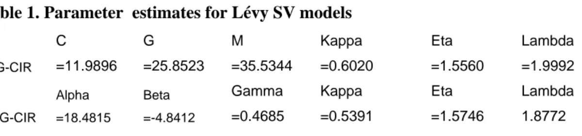
Some pricing results
For the parameters in table 1 for both the normal inverse gaussian and the variance gamma
the applet gave the corresponding results in table 2; The parameters are chosen acording to[1]
and used to calculate the prices as inddicated below.
Table 1. Parameter estimates for Lévy SV models
VG-CIR
C
=11.9896
G
=25.8523
M
=35.5344
Kappa
=0.6020
Eta
=1.5560
Lambda
=1.9992
NIG-CIR Alpha =18.4815 Beta =-4.8412Gamma
=0.4685
Kappa
=0.5391
Eta
=1.5746
Lambda
1.8772
And the initial time
y
0=
0
,
K
=
100
,
S
0=
100
,
T
=
1
year
(
250
days
),
r
=
5
%,
and the dividend
yield .
q
=
3
%
In calculating the barrier options the strike K=
(initial stock price),time to maturity
T=1(250days) and the barrier H as
0