ALGORITHMIC AND VISUAL ANALYSES FOR DISCOVERY OF ROBUST PHENOTYPE-BIOMARKER ASSOCIATIONS
by
Michael Albert Hinterberg B.S., University of Wisconsin, 2000 M.S., University of Minnesota, 2002
Graduate Certificate, Colorado School of Public Health, 2009
A thesis submitted to the Faculty of the Graduate School of the University of Colorado in partial fulfillment
of the requirements for the degree of Doctor of Philosophy
Computational Bioscience Program 2016
This thesis for the Doctor of Philosophy degree by Michael Hinterberg
has been approved for the Computational Bioscience Program
by
Carsten G¨org, Chair Lawrence E. Hunter, Advisor
Kevin Bretonnel Cohen David Kao Sonia Leach
Hinterberg, Michael Albert (Ph.D., Computational Bioscience)
Algorithmic and Visual Analyses for Discovery of Robust Phenotype-Biomarker Associations
Thesis directed by Professor Lawrence E. Hunter
ABSTRACT
Increasing availability of broad and deep biomedical data, including corresponding clin-ical and gene expression data, provides a powerful opportunity for understanding molecular mechanisms of disease and treatment response. Disease definition is based on diagnostic criteria that are subject to uncertainty, error, and change, while hypothesized phenotypes of drug response exhibit unknown effect sizes based on the particular patient characteristics. The main focus of this dissertation is to allow clinical researchers to explore multivariate clinical phenotypes and molecular mechanisms simultaneously, using interactive visual an-alytics to discover robust models of phenotype and biomarker association. Motivated by examples in heart failure and type 2 diabetes, we show the limitations of traditional analysis methods that rely on static phenotype definition. The first major contribution of this work is characterizing the disease and drug-response phenotype of heart failure using machine-learning methods, and associates phenotypes with molecular expression biomarkers. As a result, we discover a novel miRNA, hsa-miR-133a-5p, in cardiac tissue that is associated with heart failure improvement in patients treated with β-blockers. Additionally, this dis-sertation describes development of a novel, open-source, interactive visual analytics tool, “Phenotype Expression-Association eXplorer” (PEAX) that allows clinical researchers the ability to rapidly define multivariate phenotypes and statistically test for biomarker asso-ciation, with use cases in heart failure. The final major contribution is algorithms and visualization using sensitivity analysis for assessing the robustness of phenotype-biomarker associations, which differentiates between molecular associations that are highly sensitive to choice of diagnostic threshold and those that are more robustly associated. We show applications in heart failure and type 2 diabetes, both of which are chronic diseases with large health and economic impacts. Sensitivity analysis identified several additional genes
associated with cardiac reverse remodeling, and suggests a heart failure drug response sub-phenotype involving multiple heart function parameters. Compared to alternative analysis techniques, our approach improves discovery of genes associated with insulin resistance. This dissertation concludes by describing general patterns of robustness using p-curve vi-sualization that distinguish robust phenotype-biomarker associations from spurious ones. The resulting tools and methods show the importance of exploring and describing human phenotype as fuzzy variations of abnormality for biomarker discovery.
The form and content of this abstract are approved. I recommend its publication. Approved: Lawrence E. Hunter
ACKNOWLEDGMENT
I am incredibly thankful for the wonderful experience and opportunity to develop as a scientist. I could begin with all kinds of teachers from decades ago; but, knowing what I know now about good teachers, I know that they knew.
As to recent mentors, thank you to my entire committee. So much of what I have become is due to your direct mentorship, but also a significant amount from reflective observation. Dr. Kevin Bretonnel Cohen, from my first days as a student, was encouraging as to developing as a graduate student and researcher, with direct and pragmatic tips about presentations and research directions. When I saw that a person could have medical experience and linguistics and judo skills and then learn new things about biology and statistics and computer science, it verified for me that an inquisitive mind can and should always continue to pursue new knowledge even in disparate domains. Dr. Sonia Leach has showed me the importance of scientific rigor and making crisp, specific scientific claims, and I appreciate her willingness to understand overall research goals as well as attention to detail. In course lectures and preparation for preliminary exams, I have seen her approaches to teach us complex concepts through example, “doing” rather than “showing,” in a way that has informed my own teaching style. Dr. David Kao is an incredibly prolific yet modest physician and bioinformatician, and I am awed at his ability to treat patients and improve medical practice while taking the time to explain the clinical context of diseases to computationally-minded folks, treating us as scientific peers across domains. I am indebted and grateful for his encouragement, enthusiasm, and support in developing and applying new analytical methods, and his humble sharing of ideas and meaningful biological problems. Dr. Carsten G¨org opened my eyes to visual analytics, and has been consistent and unwavering in guidance toward creating meaningful tools and algorithms. With consistent feedback and support, he has helped direct me toward meaningful publications, and more memorably, I will always appreciate frank and personal discussions on many subjects. Lastly, I am grateful to Dr. Larry Hunter. Bioinformatics “didn’t exist” when I first went to school, so when I was trying to figure out how to apply longstanding interests in computer science and algorithms toward meaningful problems in human health, I was thrilled to learn about the
Computational Biosciences program right here in Colorado. He has an incredible ability to direct different, rough ideas toward a clear scientific goal, and to explain them as a compelling scientific story. He has taught me the importance of generating hypotheses that are interesting no matter which way they are proven. (Note: this is a good heuristic for making interesting choices in life as well). Through observation, I am proudly trained in keeping science open, working toward meaningful improvement of human health, and consideration of social justice and ethics in our work. These committee members have been exemplary in how to be knowledgeable and respected while also being respectful and kind towards others. With true confidence, one can focus on collaboration and support rather than competition and criticism. Thank you all for your example.
The rest of the faculty and staff have also been encouraging. Drs. Robin Dowell, Karin Verspoor, Michael Kahn, and Tzu Phang were instructive at the beginning of my research development, with rotation and class projects, and Dr. Katerina Kechris has been helpful in statistical approaches and microRNA analysis. I am very thankful to Kathy Thomas and Elizabeth Wethington for keeping many things on track, while being upbeat along the way. I appreciate current and past students and post-docs that have helped me along the way. Alex Poole and Drs. David Knox, Chris Funk, Bill Baumgartner, Meg Pirrung helped provide camaraderie when I lost my cohort. I’d like to thank the students of CPBS 7712 for participating in a wonderful teaching experience. More recently, Dr. Charlotte Siska, Dr. Gargi Datta, Laura Stephens, and Tiffany Callahan have provided helpful feedback and support. Dr. Anis Karimpour-Fard has given consistent help and suggestions, especially as I have developed biostatistics knowledge, and Dr. Elizabeth White has been kindly supportive from my preliminary examinations to the present day.
I would like to thank specific collaborators from work resulting from this research as well. In heart failure-related work, I would specifically like to thank Drs. Michael Bristow, J. David Port, Kika Sucharov, and Elaine Epperson, as well as all of the patients of the BORG trial. I would like to thank Drs. Judy Regensteiner and Jane Reusch for helping by sharing their knowledge of diabetes. I am very thankful to the National Library of Medicine Training Grant for research and program support, as well as the American Heart Association and American College of Cardiology for additional support.
I would also like to acknowledge future students as well. First, thank you for carrying the torch. And, remember to do so, because it can be dark: I have read several disserta-tion acknowledgements which acknowledge support through difficult times. Be aware and prepare, as best as one can, precisely for those times. Anxiety and depression are real risks alone, and this can be compounded by unexpected life situations. Our best bet is to steel ourselves by taking care of health and relationships. There is ample research supporting the importance of physical and emotional health. If we want others to take our scientific findings seriously, we must also do so with other health research. Do not be the cigarette-smoking physician! Rather, get outside some and laugh, get your heart rate up, and eat your vegetables: science tells us we should do these things.
Thank you to my parents for putting a Commodore 64 computer in my bedroom as a child, and for never limiting anything I wanted to read. Thank you to my extended family for support of our family during very busy times.
I am very proud and humbled by the support of our little family of three. Jessica, my dear wife, you have been by my side for 14 years of marriage. Even before that, we had a tiny apartment in Minneapolis, with our own two computer desks taking up the living room, where you might wait while I would send “one last quick email” to a student with a question in one of the labs that I taught. You were patient and supportive when I realized, later, that I still had academic curiosity and a desire to promote healthy lives – in a different way, but otherwise like you had been doing. We have had many sacrifices unfairly borne by you. But, you had more confidence and belief in me than I had in myself. Thank you for understanding me.
And, lastly, I hope I make our son Jamison proud. Jamison, you have made me re-evaluate anything I ever thought about anything. I am in awe in having so much wonder and love with us, and you have reaffirmed to me that joy and curiosity are innate, if we let them be. I am so fortunate and grateful to the program and faculty for allowing flexibility to watch you grow. It has been two years, and nothing has worn off or been taken for granted: you are an ever-present miracle. It gives me faith, then, that all of us are.
TABLE OF CONTENTS
CHAPTER
I. INTRODUCTION . . . 1
1.1 Disease Diagnosis and Phenotyping . . . 2
1.2 Phenotyping and Diagnostics . . . 4
1.3 Impact on Biomedical Research and Public Health . . . 7
1.4 Biological Background . . . 9
1.4.1 Disease Phenotyping of Heart Failure . . . 9
1.4.2 Cardiac Diagnostic Thresholds . . . 10
1.4.3 Molecular Association of Heart Failure . . . 12
1.4.4 Disease Phenotyping of Type 2 Diabetes . . . 13
1.4.5 Diagnostics in Type 2 Diabetes . . . 13
1.4.6 Molecular Association of T2D . . . 14
1.5 Dissertation Goals and Contributions . . . 15
II. COMPUTATIONAL CHARACTERIZATION OF DRUG RESPONSE IN IDCM 17 2.1 Introduction . . . 17
2.2 Data Sources and Definition . . . 18
2.3 MicroRNA Background . . . 19
2.4 Data Integration . . . 21
2.5 Methods . . . 21
2.5.1 Early Phenotype Model . . . 23
2.5.2 Gene, MicroRNA, and Phenotype Correlational Network Visualization 24 2.5.3 microRNA as Prognostic Biomarkers . . . 24
2.6 Results . . . 25
2.6.1 Early Phenotype Model . . . 25
2.6.2 Correlational Networks . . . 28
2.6.3 Baseline microRNA Prognostics . . . 29
2.7 Discussion . . . 32
III. VISUAL ANALYTICS OF MIRNA, MRNA, AND PHENOTYPE ASSOCIATION 36
3.1 Domain Background . . . 38
3.2 Analysis Task Definition . . . 40
3.2.1 Task 1: LVEF Improvement . . . 40
3.2.2 Task 2: β-Blocker Differences . . . . 41
3.2.3 Task 3: Drug Receptor Polymorphisms . . . 41
3.3 Related Work . . . 41
3.3.1 Visual Statistical Analysis . . . 42
3.3.2 Hypothesis Testing . . . 42
3.3.3 Phenotype/Group Discovery . . . 44
3.3.4 Integrated Molecular Expression Analysis . . . 44
3.4 Visual Analytics Approach and Framework . . . 45
3.4.1 Design Methodology and Infrastructure . . . 45
3.4.2 GUI Design Elements . . . 47
3.4.2.1 Binary Decision Tree . . . 47
3.4.2.2 Sliders and Histograms . . . 49
3.4.2.3 Boxplot . . . 50
3.4.2.4 Color and Highlighting . . . 51
3.4.2.5 Algorithmic Design and Performance . . . 51
3.5 Case Study . . . 53
3.6 Discussion and Lessons Learned . . . 56
3.7 Conclusion . . . 59
IV. ROBUSTNESS ANALYSIS OF PHENOTYPE-BIOMARKER ASSOCIATION 61 4.1 Introduction . . . 61
4.2 Background . . . 62
4.2.1 Diagnostic Measurement Distribution . . . 64
4.2.2 Diagnostic Error . . . 65
4.2.3 Changing Disease Definitions . . . 65
4.2.4 Disease Progression . . . 66
4.2.6 Limitations of Statistical Association Testing and “P-Hacking” . . . 67
4.3 Methods . . . 68
4.4 Results . . . 71
4.4.1 Strength of Gene Association at Different Diagnostic Cutoffs . . . . 71
4.4.2 Sensitivity and Specificity of Diagnostic Cutoff Associations . . . 72
4.4.3 Sex-Based Differential Association of T2D Genes . . . 77
4.4.4 Analysis of Molecular Mechanisms of Heart Failure Drug Response . 79 4.4.5 Robustness of Gene Association with Treated IDCM Phenotypes . . 81
4.5 Discussion . . . 83
4.5.1 Importance of Diagnostic Thresholds in Biomarker Discovery . . . . 85
4.5.2 Distribution-Dependence of Diagnostic Thresholds . . . 88
4.5.3 Visualization of Phenotype-Biomarker Robustness Patterns . . . 89
4.5.4 Meeting the Challenges of Data Exploration . . . 89
4.6 Conclusion . . . 90
V. IMPLICATIONS OF FUZZY PHENOTYPES AND ROBUSTNESS . . . 93
5.1 Introduction . . . 93
5.2 The Importance of Exploratory Phenotype-Biomarker Analysis . . . 94
5.2.1 Summary Statistics versus P-Curve Visualizations . . . 94
5.2.2 Precision Medicine . . . 97
5.2.3 Ontological Considerations . . . 98
5.3 Conclusion . . . 102
VI. CONCLUSIONS AND FUTURE DIRECTIONS . . . 104
6.1 Summary . . . 104
6.2 Future Directions and Trends . . . 105
LIST OF TABLES
TABLE
1.1 Diagnostic tests used for T2D . . . 14
2.1 Different sources of phenotype data used in BORG trial. . . 18
2.2 Three models of early drug response phenotype . . . 23
2.3 PCA-logistic regression early phenotype model . . . 25
2.4 Random forest early phenotype model features and weights . . . 26
2.5 Differentially-correlated genes in beta-blocker response . . . 30
2.6 Performance of different classifiers using baseline miRNA expression . . . 31
3.1 Common UI design elements used in framework . . . 48
3.2 Highlights from case study . . . 56
4.1 Population characteristics of T2D analysis . . . 73
4.2 Genes associated with T2D and glycemic status . . . 75
LIST OF FIGURES
FIGURE
1.1 La Femme Hydropique, painting by Gerard Dou, 1663 . . . . 5
1.2 Simulated HbA1C Distribution in Pima Indians in T2D . . . 7
1.3 Frank-Starling mechanism . . . 11
1.4 QRS complex . . . 12
2.1 Data Integration and Analysis Pipeline . . . 22
2.2 C4.5 Decision Tree classifier of drug response with 4 nodes . . . 27
2.3 C4.5 Decision Tree classifier of drug response with 2 nodes . . . 28
2.4 Baseline Correlation Networks . . . 29
2.5 Differential Gene Expression Network . . . 30
2.6 Classification accuracy of dre-miR-133a* as a biomarker . . . 31
2.7 Example miRNA Decision Trees . . . 32
3.1 Sample screenshot of PEAX . . . 39
3.2 Shiny provides reactive user-interface integration with R . . . 43
3.3 Schematic of reactivity of phenotype definition . . . 46
3.4 Design architecture of PEAX framework . . . 47
3.5 Sample outputs from task 1 use case . . . 49
3.6 Sample output from tasks 2 and 3 . . . 53
4.1 Schematic of phenotype-biomarker association for gene expression . . . 63
4.2 Schematic of phenotype-gene association testing . . . 64
4.3 Overview of stability analysis integrated into PEAX tool . . . 69
4.4 P-curve for HbA1c cutoff levels for stratifying skeletal muscle tissue . . . 71
4.5 Intersection of T2D and hyperglycemia genes by different methods . . . 74
4.6 Tradeoffs of HbA1C cutoff with ability to detect genes . . . 76
4.7 P-curve of T2D with progressively different associations . . . 77
4.8 Sex-based analysis of genes associated with glycemic status . . . 78
4.9 Gene expression patterns stratified by sex-specific HbA1c cutoff . . . 79
4.11 Phenotype definition based on QRS interval and heart rate response (HR) . . . 81
4.12 Stable Minimum P-Curve . . . . 83
4.13 Stable Plateau and Independent p-curve . . . . 84
4.14 Unstable Peak p-curve . . . . 85
4.15 P-Curves for CREBBP and HMGB3 for QRS interval and dLVEF interaction . 86 4.16 P-Curves for CREBBP and HMGB3 genes for QRS interval and HR . . . 86
4.17 CREBBP and HMGB3 association with QRS, HRR, or LVEF . . . 87
5.1 Search space of multidimensional phenotype . . . 94
5.2 An index of p-curve trends . . . 95
5.3 Diabetes and glucose abnormalities in Human Phenotype Ontology . . . 100
CHAPTER I
INTRODUCTION
Standardized disease definitions are important for medical treatment decisions and im-proving health outcomes. Despite the fact that people have been attempting to codify disease descriptions for centuries, our definition of diseases are still incomplete and chang-ing. This is because disease definition is dependent on diagnosis, which includes clinical observations as well as diagnostic measurements, which change with increased knowledge and technology. Diagnostic measurements have specific cutoff, or threshold, values used to classify disease state, and thereby define a disease phenotype. In clinical and transla-tional research, the researcher needs to define a phenotype of interest, simultaneous with discovering molecular signatures that can serve as biomarkers or insight into biological mechanism. Choosing optimal diagnostic cutoffs is challenging, and depends on the sam-ple distribution as well as characteristics of the diagnostic measurements. Traditionally, research using molecular biomarkers uses general-population disease phenotype definitions as a fixed starting point for patient stratification. However, diseases are clinically defined in ways that optimize general population treatment and billing, not necessarily mechanistic discovery.
These observations are the motivation for the work described in this dissertation, which focuses on integrated analysis of phenotype and molecular biomarkers. Through visual analytics algorithm development, specific data analysis examples and use-cases, I show the importance of exploring phenotype as a fuzzy group of concepts, rather than immutable standard. The approach, using visual analytics, shines a light on an understated problem of using the wrong definitions of disease phenotype for maximizing discovery of biomarkers. Additionally, I describe a method of showing phenotype-biomarker robustness, so as to improve phenotype models for reproducible science.
In this chapter, I describe the limitations of using a static phenotype definition model with specific, static diagnostic cutoff values, for discovery of associated molecular biomark-ers. Consequently, our ability as research scientists in translational medicine to understand new, targeted phenotypes, and associated mechanisms, is held back by the paradigm of
static clinical disease phenotypes. I describe two important, high-impact diseases – heart failure and diabetes – and how those diseases, by example, are defined in different ways by various diagnostic cutoffs. When approaching the analysis using new methods for phenotype exploration, we discover and describe additional insights into disease concepts, mechanisms, and progression.
1.1 Disease Diagnosis and Phenotyping
Appreciation for the importance of standardized disease classification, terminology, and description – collectively known as nosology – began hundreds of years ago, with physician Thomas Sydenham observing in 1675 (Walker, 1990),
All diseases should be reduced to certain definite species with the same care which we see exhibited by botanists in their description of plants...Pathological phenomena should be described with the same accuracy that a painter observes in painting a portrait.
Sydenham stresses the importance of accurate description of disease. He also harkens back even further, to Classical Greece, by artfully detailing the importance and timelessness of reliable, repeatable diagnostics:
The symptoms observed by Socrates in his illness may generally be applied to any other person afflicted with the same disease, in the same manner as the general marks of plants justly run through the same plants of every kind. Thus, for instance, whoever describes a violet exactly as to its colour, taste, smell, form, and other properties, will find the description agrees in most particulars, with all the violets in the universe.
Invoking the time of Socrates is appropriate for discussion of diagnosis, but even more so with respect to Hippocrates, the “Father of Western Medicine.” The writings of Hippocrates detail the importance of systematic examination, and combining subjective patient condition with external factors (Walker, 1990). Much later, another fundamental shift occurred at the beginning of epidemiology and medical statistics. In 19th-century London, John Snow and William Farr hypothesized and verified geographical association of cholera outbreaks and water sources, aided by improved statistical recordkeeping. Farr then suggested a
“uniform statistical nomenclature” to resolve problems of numerous regional and colloquial descriptions of disease (Moriyama, 1966).
Now, in the age of high-throughput molecular data, electronic health records, and man-aged healthcare, nosology and disease phenotype definition have advanced in importance and scope. More detailed knowledge about disease, public health, and precision medicine, have increased the granularity of disease phenotyping. Disease definitions are ultimately a main factor for treatment decisions, both at an individual and public health level. Various coding systems and ontologies provide a common definition of disease. The International Classification of Diseases (ICD), for example, is described as the“standard diagnostic tool for epidemiology, health management and clinical purpose,” and uses a hierarchy of codes for disease description (CDC, 2014). ICD has been used for decades for claims payment scheduling and justification by Medicare and Medicaid, with participation and oversight influencing development of newer ICD (Manchikanti, 2011). The current version, ICD10, contains 68,000 unique descriptive codes (CDC, 2014).
While some of the ICD codes are incredibly detailed and specific, we observe a notable increase from 13,000 codes in ICD9 (WHO, 1998). This is a reflection of a general trend of increasing sub-categorization of health status. For example, Alzheimer’s disease is fur-ther describe as early-onset, late-onset, or familial, each of which are suggestive of some differences in etiology (Sperling et al., 2011). Breast cancer is described with at least five molecular subtypes, which have implications of prognosis and treatment (Prat and Perou, 2011). Subtypes of mental health disorders are described as endophenotypes (Insel and Cuthbert, 2009), and the concept is extended to diseases like asthma (L¨otvall et al., 2011), which is now graded in ICD10 as mild, moderate, or persistent (CDC, 2014). These changes and refinements in disease classification are geared toward improved standards of care, but also increase the complexity of disease phenotyping. Since disease definition is refined over time, researchers should be aware of relying on disease state definition as a static definition, especially when data mining across studies and making comparative analyses.
1.2 Phenotyping and Diagnostics
Diagnostic measurements are an important scientific tool for assessing disease status, and have a long history of usage and change. For example, uroscopy (visual analysis of urine) dates back to Byzantine times. A doctor assessed a patient’s urine in a special flask, with detailed analysis of qualities such as color, clarity, and sedimentation. As depicted in Figure 1.1, the results of uroscopy were used, in part, to determine condition and perhaps etiology of “dropsy patients, as generalized edema was previously called (Monro, 1765). Additionally, the simple tasting of urine, and noticing an abnormal sweetness, has evolved from antiquity to modern times as a marker of diabetes (Eknoyan and Nagy, 2005). While today’s lab-based urinalysis techniques are more technologically sophisticated, disease phe-notyping and diagnostic tests are still intimately tied together.
Ideally, medicine is focused on clinical endpoints, such as reducing mortality and im-proving quality of life, such that disease states represent a noticeable impairment. However, surrogate endpoints are useful in both diagnosis and clinical trials (Weir and Walley, 2006), for standardization and convenience. Surrogate endpoints are more easily-obtained prox-ies for health, and sufficient surrogate endpoint measurements provide the same inference patterns as true clinical endpoints. Surrogate endpoints can be defined by diagnostic mea-surements, and in some cases, surrogate endpoints define diseases and syndromes entirely. For example, hyperlipedemia and hypertension, respectively, describe anormally high blood lipids or blood pressure. Both hyperlipediemia and hypertension may otherwise be asymp-tomatic, but are associated with increased morbidity and mortality risk. Correspondingly, disease diagnosis and definition is driven by clinical diagnostic measurements, with specific threshold criteria used to classify disease. A disease diagnosis is then used to inform individ-ual treatment options to improve health outcomes, and are based on standard definitions of disease. Diagnostics themselves are also aimed at improving care and health outcomes, and are improving along technological lines. Various high-throughput “-omics” measurements, imaging capabilities, and continued exponential growth in compute performance lead to exciting advancements and possibilities in detection and diagnosis of disease.
Figure 1.1: La Femme Hydropique, painting by Gerard Dou, 1663. A doctor visually analyzes a urine sample of a“dropsy” patient. (Photo in public domain)
However, all diagnostic tests are uncertain and imperfect. Diagnostic tests are evaluated based on the ability to classify disease correctly, which is generally a tradeoff between sen-sitivity and specificity. Sensen-sitivity and specificity, respectively, represent the ability of a test to detect a person who truly has a disease (true positives, “TP”), and the ability of a test to correctly discern who does not have a disease (true negatives, “TN”), versus false detection (false positives “FP” and false negatives “FN”).
Sensitivity = T P T P + F N Specif icity= T N
T P + F P
The tradeoff between sensitivity and specificity is a balance between false positive and false negative results, and are themselves dependent on the importance of a true diagnosis. And the chosen test for a diagnosis may have to do with actual cost and availability. Since various tests can be used to diagnose a disease, different sensitivity and specificity can apply to diagnosing the same disease.
Diagnostic parameters can also change over time, with new technology, knowledge of the decision, and as the precision of a given test is improved. Changes in disease defi-nitions also leads to a change in prevalence, even without any known change in current quality of life (Schwartz and Woloshin, 1998; Berlin, 2011). Diagnostic cutoffs for elevated blood pressure, for example, have changed from a systolic/diastolic measurement of 160/95 mm Hg in 1977 to 140/90 in 2003, with lower ranges of cutoffs suggested for diabetic pa-tients (Wang and Vasan, 2005). Even among papa-tients without comorbidities, diagnostic thresholds for phenotype definition also depend on population characteristics and distribu-tion of the biomarker. For example, glucose tolerance is bimodal in populadistribu-tions with high prevalence of diabetes, such as Pima Indians (and later observed in other populations), which supports validity to the definition of disease phenotype and usage of glucose toler-ance as a metric (Lim et al., 2002). Figure 1.2 shows the population distribution (top) and diabetic retinopathy prevalance (bottom) for each of 3 diagnostic biomarkers
associ-0.05$
0.15$
0.25$
6.0$
8.5$
11$
HbA1C$(%)$
Fr
e
que
nc
y
$
Figure 1.2: Pima Indians have a bimodal distribution of HbA1C. A cutoff value near the lower mode is sensitive in distinguishing retinopathy and proteinuria in patients having an HbA1C of 6.0% or more. These data are a simulation of the bimodal distribution shown in (Knowler et al., 1990) and (Barr, 2002)
ated with diabetes. While apparently correlated, each measurement still has differences in distribution. Threshold cutoff is suggested by crossover of dotted lines intersecting be-tween the two mode trajectories. In other populations, however, glucose tolerance is not as clearly bimodal (Vistisen et al., 2009). While useful and necessary for population health outcomes, general disease definition cutoffs are less specific than those derived for specific sub-populations.
1.3 Impact on Biomedical Research and Public Health
As a whole, both disease definitions and diagnostic thresholds both have a degree of uncertainty and mutability. Ideally, disease definitions are focused on improved health out-comes. However, an increasing number of disease definitions, lowered diagnostic thresholds, and additional precursor disease states (e.g., prediabetes and prehypertension) have resulted
in an observation of overdiagnosis (Moynihan et al., 2002) and medicalization (Maturo, 2012). Motivation for new disease definitions in Western societies such as the United States, especially, comes in part from social and cultural pressures (Elliott, 2004), as well as phar-maceutical development (Moynihan et al., 2002).
With disease definition and diagnostic thresholds serving multiple purposes, including population health and payment management, should we assume that a disease definition based on diagnostic thresholds are optimal for discovery in a specific clinical group or dataset? With momentum towards precision medicine and targeted therapy, we need to have more flexibility to understand diseases in the context of specific subgroups in order to further advance the right treatment for the right people. Furthermore, disease progression is associated with different gene expression profiles, as a disease is a manifestation of multiple disease processes in different affected tissues. This is challenging enough for standard disease definitions, let alone hypothesized, novel phenotypes such as drug response. For example, how much drug response, as measured by a surrogate endpoint, is “enough” to be detect molecularly as well? If a new, narrower phenotype definition is hypothesized, and associated with molecular data, how does a researcher distinguish if the phenotype definition and molecular signals are both appropriate? The distribution of clinical variables used to define phenotype is also going to be particular to a given dataset, and each variable is subject to its own degree of imprecision and uncertainty. The choice of diagnostic cutoff is important for discovery in smaller, clinical trial data. This is particularly important to exploit deep or wide data which are driven by a primary research question, in which the patients and outcome measurements were more carefully chosen for a specific question, but can serve as a rich resource for secondary research questions as well.
In the following sections, I will describe the biological background of two impactful diseases: heart failure and type 2 diabetes. Both of these diseases have challenges associated with static and hypothesized phenotype definition.
1.4 Biological Background 1.4.1 Disease Phenotyping of Heart Failure
Heart failure occurs when the heart cannot pump sufficiently to meet the body’s needs, and is a significant disease. The incidence rate is 10 per 1000 after age 65 in the United States, with a 1 in 5 lifetime risk for Americans at age 40 (Roger et al., 2011). In addition to impacting quality of life, heart failure is a costly disease, with 999,000 first-listed discharges due to heart failure, 3.4 million hospital visits, and 277,000 annual deaths (Roger et al., 2011). Heart failure is also a complex syndrome with multiple etiologies and subclassifica-tions. Heart failure can be acute (for example, following an acute myocardial infarction), or chronic. The left side of the heart may be primarily affected, resulting in reduced pumping capacity of the heart (known as systolic dysfunction); or, the right side may be affected, resulting in atrial fibrillation and irregular heartbeat (diastolic dysfunction). Associated cardiovascular comorbidities, such as hypertension and atherosclerosis, contribute to in-cidence and progression of heart failure through associated damage to the cardiovascular system. Lack of sufficient blood flow (ischemia) causes some types of heart failure. Severity of symptoms is classified in functional stages: the New York Heart Association classification system includes four progressive stages (Dolgin et al., 1994).
As heart failure develops and progresses, heart tissue changes, in a process known as cardiac remodeling. This remodeling process is evident by changes in shape, size, and function of the heart. There may be scarring and fibrosis, stiffening of the heart, and hypertrophy, as the heart tries to compensate for increased hemodynamic load. Cardiac remodeling is influenced by neurohormonal signaling, as well as genetic factors. Other organ systems are then affected by the progression of heart failure. Treatment options include lifestyle factors, such as diet and exercise; drug treatments, such as ACE inhibitors and beta blockers; and biomechanical devices, such as left ventricular assist or cardiac resynchronization devices (Remme and Swedberg, 2001). In general, treatment is built to reduce the stress on the heart to slow or reverse the worsening of symptoms. As a whole, deep understanding of heart failure diagnosis, progression, and treatment response is dependent on many different clinical measurements.
Despite the various causes for certain types of heart failure, up to half of heart failure is classified as idiopathic dilated cardiomyopathy (IDCM), which involves a damaged heart with reduced function due to unknown cause (Hazebroek et al., 2012). While the resulting symptoms of heart failure (e.g., dyspnea, fatigue, edema) may be more readily observed, further diagnosis is needed to distinguish the type of heart failure in a patient. A predomi-nant measurement for heart failure is ejection fraction, which measures cardiac efficiency as a ratio of the proportion of blood that is pumped from the ventricles. Both left ventricular ejection fraction (LVEF) and right ventricular ejection fraction (RVEF) can be observed through several diagnostic tests (Foley et al., 2012). Echocardiogram imaging is the most widely used test, with more portable and available equipment, but it requires resolution and careful interpretation. Other imaging techniques include cardiac CT (CCT) scans and cardiovascular MR (CMR). Some techniques are augmented with nuclear medicine, in which a radioactive contrast dye is introduced as a tracer for image capture. A more inva-sive technique is cardiac catheterization, in which a catheter is inserted and a radioactive contrast dye is introduced. The technique of multigated acquisition (MUGA) also uses a radioactive tracer, but it is injected via IV rather than a catheter. Each technique has var-ious additional purposes based on availability and the desire for additional cardiovascular measurements. Although there is generally high correlation between techniques, each have sources of uncertainty.
1.4.2 Cardiac Diagnostic Thresholds
LVEF has defined cutoffs for disease diagnosis. Ejection fraction is defined as the ratio of stroke volume (SV) to end-diastolic volume (EDV). Stroke volume is the change between EDV, when the heart is maximally full of blood, from end-systolic volume (ESV), which is the residual volume of blood after ventricular contraction.
EF = SV
EDV =
EDV − ESV EDV
In a healthy heart, diastolic volume increases during a phase called preload. The stretch-ing of the heart durstretch-ing this phase is directly related to the force of contraction durstretch-ing systole, as the heart delivers oxygenated blood to the body. In a heart with reduced systolic
func-tion, the stretching of the heart during preload is not matched with sufficient stroke volume during systole. This relationship is known as the Frank-Starling mechanism. As shown in Figure 1.3, when the dependence of stroke volume vs. diastole are measured in the heart, the corresponding trend describes the cardiac function.
Reduced&Systolic&Func0on& &Increased&Systolic&Func0on& Ventricular&End&Diastolic&Volume& S tr o k e &V o lu m e &
Figure 1.3: Frank-Starling mechanism. As end diastolic volume (EDV) increases during preload, stroke volume increases accordingly in a healthy heart (blue lines). In a failing heart with compromised function (red line), stroke volume is insufficiently matched to increase in EDV.
LVEF less than 40 is considered heart failure, whereas greater than 55 is normal (Ma-hadevan et al., 2008). The range in between is less established: LVEF from 40-50 is often considered reduced ejection fraction. The remaining range of 50-55 is less well-defined (Ma-hadevan et al., 2008). Sometimes additional cutoffs are defined, such as a lower LVEF cutoff of 25 being used for LVAD eligibility (Mancini and Colombo, 2015). Furthermore, once a treatment is administered, and LVEF is monitored for improvement, one needs to define cutoffs for responsiveness. Therefore, various thresholds for LVEF, which itself can be measured using several diagnostic techniques, can be used to stratify patients in different meaningful ways for testing specific hypotheses on heart failure.
An additional cardiac diagnostic is the width of the QRS complex, shown in Figure 1.4. Based on the conventional labeling of events on an electrocardiogram, the QRS complex is
visible as a pattern of spikes representing depolarization of cardiac cells. A narrow QRS width of less than 100ms is generally associated with healthy patients, whereas wider QRS intervals of 120ms or more are generally deleterious. In the BORG study, QRS interval width was found to be associated with drug responsiveness.
P"
Q"
T"
R"
S"
QRS"Complex"
Figure 1.4: QRS complex. An electrocardiogram measures heart conduction. Notable changes in electroconductivity are labeled P,Q,R,S and T. Rapid depolarization (a shift in charge distribution) is shown as a pattern known as the QRS complex. The width of this complex, in milliseconds, varies depending on cardiac health.
1.4.3 Molecular Association of Heart Failure
Because of the complexity of heart failure, numerous molecular mechanisms have been hypothesized and identified with respect to cardiac remodeling. Understanding of the molec-ular mechanisms associated with heart failure is also correspondingly complex. Molecmolec-ular mechanisms associated with heart failure include neurohormonal signaling pathways and associated receptors, vasculogenesis, and angiogenesis. Cardiomyoctes may be affected through mechanisms related to proliferation, apoptosis, hypoxia and hypertrophy (Hilfiker-Kleiner et al., 2006). Energy transport and metabolic processes in the heart are also influ-enced, as energy substrate in the heart changes during disease progression. Cardiac conduc-tion is affected through ion channels (namely potassium, sodium, and calcium). Proteins
such as myosin are important for muscle contractility in the heart. These are just some known examples, but there are other important molecular effects involving other systemic (e.g., immune and inflammation response) and organ responses as the body compensates for reduced heart function.
1.4.4 Disease Phenotyping of Type 2 Diabetes
Type 2 Diabetes (T2D) is a costly disease of increasing prevalence in the United States and worldwide (CDC, 2012). This is a chronic condition in which the body is unable to process glucose normally, as insulin production and utilization in the body is impaired (As-sociation and Others, 2006). A condition of prediabetes is a less pronounced type of insulin resistance, but is considered a precursor that is likely to progress to diabetes if left uncon-trolled (Nichols et al., 2007). T2D is influenced by lifestyle factors, and can be mitigated or prevented through diet and exercise interventions (Smyth and Heron, 2006). T2D is additionally influenced by genetic factors, with high concordance of diabetes prevalence in identical twins, and a marked increase in risk with family history of T2D. Demographically, certain populations are notably more at risk for T2D (Lim et al., 2002). Left uncontrolled, type 2 diabetes leads to pathological microvascular and macrovascular issues, including serious problems of neuropathy, nephropathy, and retinopathy (Root et al., 1954).
1.4.5 Diagnostics in Type 2 Diabetes
T2D diagnosis and treatment can be measured through several clinical diagnostic tests. A random plasma glucose test can reveal serious T2D if blood glucose is abnormally high. Otherwise, a fasting plasma glucose (FPG) assessment measures blood glucose in a fasting condition, while an oral glucose tolerance test (OGTT) measures insulin response to glucose after a fix period (2 hours) of time (Nathan et al., 2007). Glycated hemoglobin levels can be measured (HbA1C) as a proxy for the average glucose levels over the previous few months (Nathan, 2009). Each respective test has a defined threshold for diabetes diagnosis, and in recent years, a diagnosis of prediabetes as well. T2D is diagnosed with an initial and confirmatory test both exceeding respective thresholds.
Each test has advantages and disadvantages with respect to cost and convenience, as well as specificity and sensitivity tradeoffs. OGTT and FPG measure glycemic response, which is
Table 1.1: Diagnostic Tests Used for T2D
Test Type Description Details
RPG Random Plasma Glucose Convenient Highly variable
FPG Fasting Plasma Glucose More accurate than RPG
Only measures non postprandial state Requires fasting compliance
OGTT Oral Glucose Tolerance Test Measures post-prandial response Lengthier clinic visit
HbA1C Glycated Hemoglobin Measures metabolic effects from previous 8 -12 weeks
Does not measure direct glucose response
integral to diabetes definition itself (Nathan et al., 2007). OGTT has higher sensitivity, but requires a lengthier medical visit and implementation. FPG is a more convenient measure of glycemic response, but measurement of fasting glucose level may not as realistically capture an individual’s typical post-prandial state. HbA1C has been more commonly used recently as the primary diagnostic tool for T2D. It has advantages of essentially representing the average state of the body over the previous 8-12 weeks. However, HbA1C truly measures protein glycation in the body, so it is a proxy measurement for glycemic response, and known to be confounded by demographic factors such as age and ethnicity (Pani et al., 2008).
1.4.6 Molecular Association of T2D
T2D is associated with various aspects of insulin receptivity and signaling. Addi-tional pathways are affected during the course of disease, such as hemodynamic path-ways involved in plasma and solute levels (regulated by renin, angiotensin, and aldos-terone) (Cooper et al., 2007). Oxidative stress is increased, as are levels of pro-inflammatory cytokines (Evans et al., 2003). Additional outcomes from diabetes progression, such as renal fibrosis, glomerular hypertrophy, nephropathy, and retinopathy, are associated with various associated changes in gene expression (Arora and Singh, 2013).
1.5 Dissertation Goals and Contributions
The main focus of this dissertation is to allow clinical researchers to define, explore, and understand multivariate clinical phenotypes and associated molecular mechanisms si-multaneously. With algorithms that support interactivity and visualization of robustness, the provided tools and methods move beyond relying on static phenotype definition and statistical p-value of association, toward developing robust, comprehensive, data-driven phenotype and biomarker models. This work was motivated primarily by clinical investi-gation of IDCM and T2D, and provides discovery and definition of complex phenotypes in several ways. In Chapter 2, I show both unsupervised and supervised machine-learning techniques applied to a clinical dataset comprised of IDCM treated with beta blockers, including multidimensional aspects of time, clinical variables, and gene and miRNA expres-sion. I show the results of several methods of feature selection and resulting correlating network are shown, to characterize the general phenotype of beta-blocker responsiveness in heart failure. Still, a single J48 decision tree outperformed alternative machine learn-ing methods, and suggested a novel microRNA, miR-133a-5p, is predictive of beta blocker response. This result was presented and shared as an abstract (Hinterberg et al., 2013). In Chapter 3, I then present the problem of fuzzy, complex phenotype definition, in which clinical variable thresholds of importance are unknown. To address this problem, we present a visual analytics tool, PEAX (Phenotype Expression Association eXplorer), which allows interactive definition and testing of phenotype association with expression biomarkers. A use-case study suggests that interactivity, responsiveness, and visual representation of phe-notype and data distribution facilitates discovery and collaboration from expert domain users, without requiring a dedicated statistical analyst. We contributed these insights to the bioinformatics and visual analytics community, as well as open-source publishing and access of the tool (Hinterberg et al., 2015). In Chapter 4, I provide a method for analyzing the stability of complex phenotype associations with expression biomarkers. We discover visualization patterns that rapidly and interactively distinguish between stable, spurious, and independent phenotype-expression associations. Our visualization of p-curve patterns improve upon traditional p-value-based ranking of gene associations by providing additional information about groupwise and individual gene association robustness. By applying
sta-bility analysis to a heart failure dataset, we discover a novel, stable phenotype of beta blocker responsiveness involving QRS interval and heart rate reduction. Additionally, we describe analyses of a public T2D dataset, and show that analyzing stability as well as differ-ent diagnostic cutoffs for disease definition detects additional genes associated with insulin resistance compared to the original study. These results are being submitted for review. In Chapter 5, I place these results against current trends, and speculate upon the meaning of p-curve patterns. I then summarize and conclude the previous work, with suggestions on future directions.
CHAPTER II
COMPUTATIONAL CHARACTERIZATION OF DRUG RESPONSE IN IDCM1
2.1 Introduction
As described in the Introduction, idiopathic dilated cardiomyopathy (IDCM) has a varying degree of responsiveness to treatment with beta-blocking agents, some some patients seeing improvement in heart function after treatment, but not others. Left ventricular ejection fraction (LVEF) is a useful metric for capturing the reduced systolic functionality of a failing heart, and change in LVEF serves as a surrogate endpoint for beta-blocker response (Lowes et al., 2002). During heart failure, the heart remodels pathologically; improvement in heart function of the failing heart is known as reverse remodeling. With more diagnostic observations, we are able to characterize the phenotype of IDCM and drug response in more detail. Combined with molecular expression data, we hypothesized that we could discover sub-phenotypes and predictors of reverse remodeling in IDCM.
This hypothesis was investigated in the clinical trial on the “Effect of β-blockers on Structural Remodeling and Gene Expression in the Failing Human Heart (BORG)” (Clini-calTrials.gov, 2013). In this study, subjects were enrolled with idiopathic dilated cardiomy-opathy (IDCM), presenting with a compromised LVEF < 40%. This type of IDCM is known as systolic heart failure, and approximately 60–70% with this disease have been shown to re-spond to β-blocker treatment (Bristow, 2000). Patients enrolled in BORG were randomized to one of three different β-blocker treatments: carvedilol, metoprolol, or motoprolol plus doxazosin. The patients were monitored for up to a year from initial treatment; they exhib-ited a variable improvement in LVEF with β-blocker treatment as observed previously (In-vestigators, 2001). Biopsies from ventricular tissue for each patient were performed prior to β-blocker treatment and at 3 and 12 months; myocardial gene expression of ∼ 34, 000 hu-man mRNAs and ∼ 7800 miRNAs was measured, using Affymetrix microarrays, producing 1Portions of this chapter were previously published as Myocardial expression of the microrna
dre-mir-133a-5p is associated with improvement in left ventricular ejection fraction in patients with idiopathic dilated cardiomyopathy treated with beta-blockersin Journal of the American College of Cardiology 61:10 (page E714), March 2013 and is included with the permission of the copyright holder
longitudinal in vivo whole-transcriptome gene expression data in human IDCM patients. The clinical outcome used to measure drug response was improvement in LVEF, and the primary aim of the study was to understand molecular mechanisms of LVEF improvement with β-blockers and to identify predictive clinical and/or molecular biomarkers to predict LVEF improvement. A panel of genes, generally indicative of fetal-vs.-adult gene program-ming, was discovered through a traditional statistical analysis using Wilcoxon signed-rank testing of gene expression fold-changes differentially expressed between drug-responders and non-responders (Kao et al., 2015).
In this chapter, we describe additional machine learning-based techniques for character-izing the phenotype of beta-blocker response in IDCM patients, based on broad patient and molecular data. We also describe analysis of microRNA expression as prognostic indicators of beta blocker response.
2.2 Data Sources and Definition
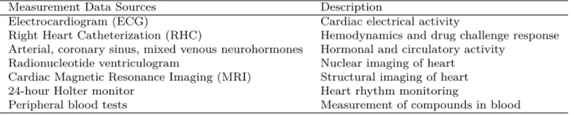
In this section, I will describe the BORG dataset analyzed in this chapter, and used for several later examples as well. Clinical data includes demographics, medical history, inva-sive hemodynamics, drug challenge measurements, myocardial histology, peripheral blood tests, neurohormone measurements, cardiac MRI, 24-hour Holter monitor, and radionu-clide ventriculograms, as well as genotyping for three different adrenergic receptor single nucleotide polymorphisms (SNP). Combined, this feature set comprised thousands of fea-tures per patient, including both discrete and continuous variables.
Clinical data were available from several sources, with a summary of their purposes shown in Table 2.1.
Table 2.1: Different sources of phenotype data used in BORG trial.
Measurement Data Sources Description
Electrocardiogram (ECG) Cardiac electrical activity
Right Heart Catheterization (RHC) Hemodynamics and drug challenge response
Arterial, coronary sinus, mixed venous neurohormones Hormonal and circulatory activity
Radionucleotide ventriculogram Nuclear imaging of heart
Cardiac Magnetic Resonance Imaging (MRI) Structural imaging of heart
24-hour Holter monitor Heart rhythm monitoring
Additional demographic data (such as age and sex), as well as body composition data, were also available for each patient. Categorical (e.g., type of drug administered; biological sex) were discretized. Some clinical data at various timepoints were missing, which were handled in several different ways, discussed later in this chapter. mRNA expression was quantified using Affymetrix HGU-133a, which includes 33686 gene probesets, as well as the Affymetrix GeneChip MiR, comprised of 7815 microRNA probesets. Microarray expression data were normalized using log-scale robust multi-array (RMA) analysis.
2.3 MicroRNA Background
The BORG dataset is a wide dataset consisting of many covariates for each sample. In the Introduction, we described the phenotype characteristics of IDCM. The BORG data in-cludes expression data on both messenger RNA (mRNA) and microRNA (miRNA, or miR). mRNA encodes amino acid sequence information necessary to produce proteins. However, mRNA may be post-transcriptionally modified or regulated such that it does not always translate into proteins. microRNA binding is one potential mechanism of mRNA regulation, which will be described here in more detail.
microRNAs are much shorter sequences of RNA, generally around 22 nucleotides in length. Instead of coding for proteins, microRNAs are generally observed to have a regula-tory function, often repressing specifically targeted genes. microRNAs are short, noncoding sequences of RNA with a regulatory function. miRNAs have a seed sequence region of around 6-8 nucleotides, which are complementary to an mRNA target sequence. miRNAs repress translation of a target mRNA, effectively silencing specific mRNA. Therefore, the interaction of miRNA and mRNA together better captures biology.
The source of miRNA can be exogenous, but miRNA is generally transcribed by miRNA genes. After transcription as a primary miRNA (pri-miRNA), the transcript is processed into a pre-miRNA and exported to the cytoplasm. The pre-miRNA is cleaved into a comple-mentary pair of double-stranded miRNAs by the enzyme Dicer. The resulting pair includes a functional regulatory strand of 22-23 nucleotides. This primary strand is incorporated in to the RISC complex with the target mRNA and other associated proteins. The other
strand of the miRNA is called the passenger strand, and is generally thermodynamically unstable, not incorporated into the RISC complex, and is degraded.
miRNA are important markers of human health and disease, and differences in miRNA expression are known to be tissue-specific (Babak et al., 2004). They can be administered as therapeutic agents (van Rooij and Kauppinen, 2014), serve as biomarkers associated with disease progression (van Rooij and Olson, 2007), as well as drug-responsiveness (Mishra and Bertino, 2009), meaning that microRNA-mRNA association is of high interest to re-searchers. microRNA can therefore be used as predictors of disease risk and drug response. For example, in heart failure, specific miRNAs associate with cardiac hypertrophy and re-modeling, as well as related disease processes like fibrosis, and cellular proliferation and apoptotic processes (Melman et al., 2014). miRNA function is tested experimentally in mouse knockout models, in which specific miRNAs are over- or under-expressed compared to controls, and associated with hypothesized effects.
High-throughput profiling of miRNA (Dedeo˘glu, 2014) allows comparable methods and approaches as mRNA quantification. Because of the regulatory nature of miRNAs and association with target mRNA, the combination of miRNA and mRNA expression provides insight into disease mechanisms. Conversely, knowledge about existing genes and gene networks, as well as sequence homology, helps to inform and direct hypotheses regard-ing unknown miRNAs. For example, mirBase is a publicly-accessible database of miRNA knowledge, including observed sequences and links to experimental information (Griffiths-Jones et al., 2006). The overall model of miRNA regulation is well-suited to bioinformatics analysis techniques. The critical points of a general bioinformatics model are generally straightforward, using the following observations:
1. miRNA has an important seed sequence of 22-23 base pairs 2. miRNA is complementary to mRNA target sequences 3. Quantified miRNA expression correlates with function
4. miRNA expression is generally anticorrelated with mRNA target expression
5. miRNA-mRNA interaction can be experimentally verified, and captured in a knowl-edge base
6. Novel miRNA-mRNA targeting can be hypothesized based on sequence (through ther-modynamic models, sequence homology, etc.)
Given that microRNAs are known to be involved in regulation of cardiac hypertrophy and remodeling, we hypothesized that their differential expression may be predictive of prognosis and treatment response. To test this hypothesis, improvement in LVEF over the course of one-year of beta-blocker treatment was correlated with baseline myocardial microRNA expression in heart failure patients.
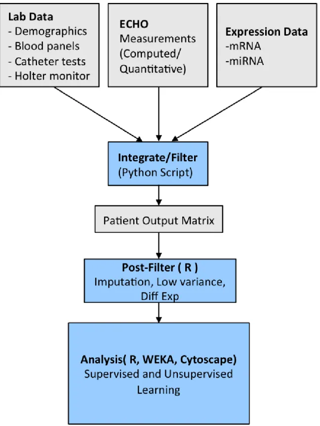
2.4 Data Integration
Since these data were from different sources, the only thing they shared in common was patient number. In order to integrate the data, data inputs were initially pre-processed from independent data files that stored clinical measurements or expression values anno-tated by date or timepoint, pertaining to unique, de-identified patient ID’s. Clinical source data were provided as comma-separated variable (CSV) files with unique patient identi-fier numbers, labeled clinical measurements, measurement value, and date of exam. This was processed by developing a custom Python script to determine the baseline date and to separate measurements into baseline, 3-month, or 12-month followup, respectively. This was used to generate an aggregate patient matrix which included patient identifier in each row, and unique measurements in each column. Missing data were left as blank values, and clinical measurements with at least 25% missing values were not included in analysis.
2.5 Methods
We developed and tested 3 different types of models for characterizing IDCM and reverse remodeling using phenotype and expression data. Generally, these models include “early phenotype” characterization of beta-blocker response; visual correlational networks; and miRNA prognosticator models.
2.5.1 Early Phenotype Model
Drug response in the BORG trial was defined by LVEF improvement after 12 months for most patients. However, patients also had a 3 month follow-up appointment. We hy-pothesized that a phenotype based upon clinical measurements from the first 3 months (including baseline) could serve as a proxy for overall beta blocker response. The implica-tions of defining an earlier endpoint would be to determine beta blockers earlier in time, thereby directing treatment decisions appropriately. We developed three models for early representation of drug response phenotype, shown in Table 2.2:
Table 2.2: Three models of early drug response phenotype Phenotype Model Model Type
PCA+Logistic Regression Unsupervised Random Forests Supervised C4.5 Decision Tree Supervised
In order to determine the clinical features most associated with beta blocker response, we performed PCA on clinical phenotype data including baseline and 3-month followup measurements. This step is known as feature selection, to reduce the space of potential phenotype features dramatically. We used the features selected in the first PCA component to build a logistic regression model, both with and without interactions. This is a form of unsupervised learning, as we did not provide drug response classification information as inputs to the model. Instead, this is intended as a data-driven characterization of the phenotype feature space. We also built additional models using random forests, again built upon baseline and 3-month followup clinical measurements. Random forests are supervised models, attempting to maximize information gain by splitting of randomly-selected feature nodes, with resulting iterations weighted as an ensemble. Finally, we built models using C4.5 decision trees, for comparative performance and simplicity of model interpretation.
In this way, we can compare the features selected by unsupervised and supervised learning, and measure how well the early phenotype models can serve as a proxy for 12-month drug response.
2.5.2 Gene, MicroRNA, and Phenotype Correlational Network Visualization The BORG dataset includes clinical data, mRNA expression, and microRNA expression data. In order to use these different datasets to analyze potential molecular mechanisms as-sociated with IDCM and drug response, we analyzed correlation between these data types in several different ways. We included diagnostic measurements, mRNA expression, and miRNA expression values as candidate features. We chose Cytoscape (Shannon et al., 2003) to visualize correlational networks, to make the correlational networks easier to inter-pret. This way, we could see linkages between hubs and nodes that are mutually correlated with intermediate features. We chose a cutoff of 0.8 to visualize highly-correlated features. We defined two different models for baseline correlation: a mRNA-miRNA network, and a phenotype-expression network. The aim of both of these is to test the hypothesis that base-line signals associated with heart failure can be detected in a correlation network. Missing phenotype data were imputed using kNN imputation, and we limited molecular features to the highest 8000 variant signals. Additionally, we defined a differential expression network of mRNA expression between 0 and 12 months. We limited expression analysis to genes differentially expressed (Mann-Whitney test) between responders and non-responders, and visualized the gene change network. We hypothesized that genes with correlated changes would be enriched for biological processes related to reverse remodeling.
2.5.3 microRNA as Prognostic Biomarkers
Using normalized baseline microRNA expression, we evaluated 3 different classifiers in Weka, and their respective ability to discriminate between responders and non-responders: C4.5 Decision Trees, Random Forests, and Sequential Minimal Optimization (SMO). We chose the three classifiers based on tradeoffs of simplicity and interpretability, expected validation robustness, and classification accuracy. The C4.5 algorithm (Quinlan, 1993) iterates through features to maximize information gain at each splitting step when creating a decision tree. The random forest algorithm is an ensemble of decision trees (Ho, 1998), in which different decision trees are constructed, and the consensus (mode) classification is used as the result. As an ensemble, random forests thereby reduce overfitting or bias of a single decision tree, but at the expense of simplicity in human readability. SMO is an
algorithm for training support vector machines (SVMs), which are classifiers that maximize separation of distinct classes via a discriminatory hyperplane. Discrimination by usage of a hyperplane allows a high-dimensional feature space to be mapped into lower dimensions, and usage of non-linear kernel functions in SVMs allows for a non-linear classifier.
We evaluated C4.5, Random Forests, and SMO using Leave-one-out Cross Validation (LOOCV). LOOCV involves training a model built upon all but one instance, evaluating on the withheld instance, and recording the result; then, iterating through all other instances and testing in the same way. The combined result reflects the validity of the overall model. We chose LOOCV because the modest number of training samples (34) precludes partition-ing of sizeable trainpartition-ing and test sets. In contrast, the sample size is also small enough to risk appreciable overfitting.
2.6 Results
We show the results of the different models created and tested, below. Due to the different types of models testing, discussion occurs along with model results.
2.6.1 Early Phenotype Model
The early phenotype model, built as a logistic regression model using PCA feature selection for a logistic regression model, is shown in Table 2.3. Nine features define a simple logistic regression model, and the top five were used for a model with interactions.
Table 2.3: PCA-logistic regression early phenotype model
Feature Time Weight Linear Interactions
MUGA LVEF 3 months 1.000 + *
ECHO LVID(s) 3 months 0.959 + *
ECHO LVID(d) 3 months 0.925 + *
ECHO ESV (Teich) 3 months 0.906 + *
ECHO ESV (Cubed) 3 months 0.894 + *
ECHO LVID(d) baseline 0.882 +
ECHO EDV(Teich) 3 months 0.879 +
MUGA ESV baseline 0.872 +
ECHO EDV (Cubed) 3 months 0.869 +
MUGA LVEF at 3 months was the highest loading feature in an unsupervised model using PCA. This is interesting, because it suggest an appreciable variance of LVEF at 3 months. MUGA LVEF at 3 months, alone, predicts 27 of 35 (77%) response statuses correctly (of those with 3-month MUGA LVEF values; data not shown). Also, most mea-surements (7 out of 9) used in this model are 3 month meamea-surements, suggesting higher variation than at baseline. In this model, ECHO measurements are highly variable, and are able to distinguish when interactions are considered. This suggests morphology of reverse remodeling is measurable through echocardiograms.
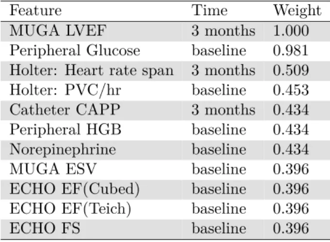
We tested an additional early phenotype model of beta-blocker response in IDCM using random forests. The features and feature importance weight are shown in Table 2.4.
Table 2.4: Random forest early phenotype model features and weights
Feature Time Weight
MUGA LVEF 3 months 1.000
Peripheral Glucose baseline 0.981 Holter: Heart rate span 3 months 0.509 Holter: PVC/hr baseline 0.453 Catheter CAPP 3 months 0.434 Peripheral HGB baseline 0.434 Norepinephrine baseline 0.434
MUGA ESV baseline 0.396
ECHO EF(Cubed) baseline 0.396 ECHO EF(Teich) baseline 0.396
ECHO FS baseline 0.396
Similar to the previous unsupervised models, MUGA LVEF at 3 months is most infor-mative of beta-blocker response in a random forest model. With random forests, however, we observe a more distributed mix of baseline and 3-month measurements, as well as a combination of different lab biomarkers, imaging, and heart monitoring. Under this model, the different clinical sources are important, and the results suggest that prediction is not dominated by certain technology or type of data. These results suggest that disparate types of data at both baseline and followup have contributory explanatory value in the reverse remodeling phenotype.
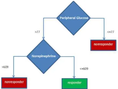
We also generated simpler classification models of early phenotype using C4.5 decision trees using baseline measurements. The goal was to discover a combination of baseline features associated with drug response that could be readily interpreted by clinicians. Two of the most accurate classifiers are shown in Figure 2.2 and Figure 2.3. Different trees were created through parameter exploration; namely, changing the minimum number of leaf instances to avoid overly deep trees and overfitting.
Figure 2.2: C4.5 Decision Tree classifier of drug response with 4 nodes. “Mildly Dilated LA” refers to dilated left atrium observed as an echocardiogram impression. Peripheral glucose refers to circulating blood glucose; MUGA stroke volume is a cardiac function parameter; 138-sodium is a normalized value of sodium measured in the blood.
The decision tree models for baseline classification show glucose, sodium, and nore-pinephrine measurements being important, in addition to an echocardiogram impression of “mildly dilated LA” (binary coded). These models are simpler to describe clinically, and the lab measurements are less invasive to obtain. However, even the simpler 2-node model, based on glucose and norepinephrine levels, is not robust to LOOCV, with 45%
classifica-Figure 2.3: C4.5 Decision Tree classifier of drug response with 2 nodes. Peripheral glucose refers to circulating blood glucose; norepinephrine is measurement of the hormone norepinephrine in the blood.
tion accuracy. Still, to evaluate whether the cutoffs for glucose and norepinephrine were predictive of beta-blocker response, we evaluated these cutoffs on another dataset. The Mul-ticenter Oral Carvedilol Heart Failure Assessment (MOCHA) trial enrolled patients that were treated with carvedilol (Bristow et al., 1996). We did not see concordance of response in MOCHA based on glucose and norepinephrine levels.
2.6.2 Correlational Networks
The results of the baseline correlational network between baseline miRNA and mRNA is shown in Figure 2.4. The baseline miRNA network shows a “hairball” of genes and microRNA. We see that miR-100 and various homologs are highly correlated, which makes sense because the probe sequences are the same or very similar. However, none of the correlated genes are known or predicted targets of miR-100. 3 of the 6 correlated genes (CORO1A, CD4G, and NKG7) are localized in the plasma membrane, but otherwise do not suggest a metabolic process related to IDCM.
The small sub-network of phenotype and expression in Fig 2.4b shows correlation be-tween right ventricular diastolic diameter, pulmonary arterial systolic pressure, and the gene TNC. The TNC gene codes for Tenascin-C, which localizes to the extracellular matrix dur-ing damage and repair processes. Hessel et al. (2009) found that TNC is upregulated durdur-ing right ventricular pressure overload: increased right ventricular diastolic diameter and PASP
Figure 2.4: Correlation networks visualized in Cytoscape. a) mir-100, and homologs, are correlated with several genes, including HOXB4, CORO1A, CD3G, LAIR2, NKG7, SIAE. b) In a phenotype-expression network, a small subnetwork shows association between catheter pulmonary arterial systolic pressure (PASP), right ventricular diastolic diameter (RVDd), and the gene TNC.
would indicate these conditions. This sub-network was a noticeable visual outlier among other less-clear network associations. As a whole, our findings recapitulated Hessel’s obser-vations, and verified that a correlational model combining phenotype and gene expression, using visualization, could direct a meaningful biological finding.
A differential gene correlational network, showing genes differentially-expressed between responders and non-responders, is shown in Fig 2.5. Again, this subnetwork was found by visual inspection of standalone correlation networks in Cytoscape. Of these genes, a DAVID analysis shows that 7 of the 14 are annotated for glucose metabolism, insulin sensitivity, and/or T2D (see Table 2.5).
2.6.3 Baseline microRNA Prognostics
In Table 2.6, we present best performance, with some parameter space exploration, of the three different classifiers on baseline miRNA expression for prediction of beta blocker response.
Surprisingly, C4.5 decision tree outperformed the other two classifiers. Even more surprisingly, the best-performing C4.5 tree involves a single miR, dre-miR-133a*, that best