Classification of groundwater based on irrigation water quality index and GIS in Halabja Saidsadiq basin, NE Iraq

JOURNAL OF

ENVIRONMENTAL HYDROLOGY

Open Access Online Journal of the International Association for Environmental Hydrology

VOLUME 24

2016

CLASSIFICATION OF GROUNDWATER BASED ON IRRIGATION

WATER QUALITY INDEX AND GIS IN HALABJA SAIDSADIQ

BASIN, NE IRAQ

Salahalddin S. Ali2

Nadhir A. Al-Ansari3

Sven Knutsson3

1_{Department of Geology, University of Sulaimani, Kurdistan}

Region, NE. Iraq

2_{President of University of Sulaimani, Kurdistan Region, NE.}

Iraq

3_{Department of Civil, Environmental and Natural Resources and}

Engineering, Lulea University of Technology, Sweden

Assessment of groundwater for irrigation purpose is proposed using the Irrigation Water Quality Index (IWQI) within the GIS environment. The model was applied to several aquifers in the study basin. Water samples were collected from thirty-nine sites from both water wells and springs from the dry season (September 2014) and the wet season (May 2015). Samples were tested chemically and physically for several variables: EC, Ca+2_{, Mg}+2_{, Cl}-_{, Na}+ _{and HCO3}- _{and SAR. The accuracy and}

precision methods were applied to find out the uncertainty of the chemical analysis results and its validity of application for the geochemical interpretations. Based on the spatial distribution of IWQI, the groundwater quality of HSB classified into several classes of both dry and wet seasons in terms of its restrictions on irrigation purposes. The classes include, Severe Restriction (SR), High Restriction (HR) and Moderate Restriction (MR). The coverage areas of all three classes are 1.4%, 52.4% and 46.2% for the dry season and 0.7%, 83.3% and16% for wet seasons respectively. The considerable variations in all these classes have been noted from dry to wet seasons, this might be related to increasing the aquifer recharges from precipitation and decreasing the aquifer discharges by the consumers in the wet season. Then the model was validated based on the relation between the aquifer recharge and spatial distribution of IWQI, the result of this validation confirmed the outcome of this study.

INTRODUCTION

Many regions particularly in the arid and semi-arid regions in the world are explicitly dependent on groundwater as one of the main water resource. The study area is located in the NE part of Iraq, called the Halabja Saidsadiq Basin and referred to in this paper as HSB (Figure 1). Groundwater is considered to be one of the most important sources of water providing water for agricultural activity, drinking and industrial activities (Abdullah et al., 2015). Previously, this area has been destroyed by army attacks by chemical weapons. So the area is facing significant economic development and improved security after 2003. Several factors that lead to an increase in demand for potable water in the past few years are population growth, socioeconomic development, technological and climate changes (Alcamo et al. 2007). Consequently, water quality controls the management and irrigation leaching elements, as well as in the water treatment, so as to achieve an extraordinary level of production in situations where irrigation systems are used (Castellanos et al., 2002).

Irrigation and agriculture considered to be the most intensive water consumer and it required 66% of demand across the region (Hiniker, 1999 cited in Hussain et al., 2014 ) and consequently the problem of water shortage problem cannot be accurately analyzed without a thorough consideration of agriculture in the region (Sadik and Barghouti, 1994).

The quality of water is labeled in terms of its chemical, physical and biological characters. Before using the water, it is important to establish its quality of numerous purposes such as drinking, agricultural frivolous and industrial utilizes (Sargonkar and Deshpande, 2003; and Khan et al., 2003). In HSB, the groundwater quality has mainly established huge consideration since water of high quality is required for domestic and irrigation needs. Up to date, in HSB groundwater assessment has been based on laboratory investigation only, but the arrival of Geographical Information System (GIS) and satellite images has made it very easy to assimilate several databases. GIS is a powerful tool for evolving interpretations and solutions for many water resources problems, evaluating water quality, determining water availability, sympathetic the natural environment, averting flooding, and for managing water resources on both local and regional scales (Ferry, et al., 2003).

Water quality indexes to give a single number that articulate overall assessment of water quality of assured sites and time based on several parameters of water quality. The goal of an index is to revolve multifaceted data onto water quality of more comprehensible information and simple utility by the public. However, as claimed by (Yogendra and Puttaiah, 2008), a water quality index supported by a number of extremely significant parameters can supply an uncomplicated indicator of water quality.

Water Quality Index (WQI) is commonly applied to qualify urban water supply, it has been extensively used by environmental planning decision makers. So, it is important to assess the quality of the irrigation water in order to eliminate or diminish negative impacts on agriculture (Mohammed, 2011). Therefore, several different classifications in the world have been proposed to evaluate the irrigation suitability of water. Richard classification which depended on Sodium Absorption Ratio (SAR) and electrical conductivity (EC) (Richards, 1954 cited in Hussain et al, 2014). A further classification which is based on sodium percentage concentration (Na %) and its relationship to EC , was proposed by (Wilcox in 1955). Beside these, Ayers and Westcot in 1999, recommended another classification based on the hydrochemical changes of salinity, nutrients concentration in (ppm) , cations and anions in (epm) and miscellaneous influences. Finally Don in 1995, proposed a new classification based on some more parameters as previously recommended, this type of classification is based on SAR, EC, %Na and TDS. Furthermore, it is being important to mention that, there are different

requirements among different sites for irrigation water quality, this differentiates based on the cultivated crop pattern, the regional soil and climatology conditions (Babiker et al. 2007).

From the previously mentioned historical background, mapping of irrigation water quality is considered to be an expensive instrument for the assessment of spatially dispersed of entity quality parameters. Accordingly, GIS with a sufficient database provide a vital podium for maps envisaging and creating comparative assessments, evaluating water quality, developing solutions to water resource problems, and agriculture development from its tool of decision making (Arsalan, 2004).

In the current study area, the groundwater quality assessment for the irrigation purpose has not been done yet; it might be effect on the quality and the quantity of the irrigation and agricultural products. Therefore, the main goal of this study are to apply the Irrigation Water Quality Index (IWQI) with GIS as the first attempt on the region for (1) evaluating the status of groundwater quality and its suitability for irrigation function; (2) to set up the spatial distribution of groundwater quality parameters; and (3) to generate a map of groundwater quality.

STUDY AREA

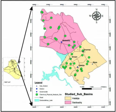
HSB is located in the northeastern part of Iraq and geographical coordinate value ranged between the latitude 35” 00’ 00" and 35" 36’ 00" N and the longitude 45” 36’ 00" and 46” 12’ 00" E (Figure 1).In terms of hydrogeological characteristics the area is divided into two sub-basins including Halabja-Khurmal and Said Sadiq sub-basins by Ali (2007). The whole covered area of HSB is about 1278 square kilometers with an approximate population of 190,727 in early 2015 based on the data achieved from Statistical Directorate in Sulaimaniyah. Meteorologically, this area is characterized by a distinct continental interior climate of hot summers and cold winters of the Mediterranean type with the average annual precipitation ranging from 500 to 700 mm. About 57% of the studied area classified by an arable area due to its suitability for agriculture purposes. Therefore, both fertilizers and pesticides are extensively used in this area, so it affects the groundwater quality as mentioned by (Huang et al., 2012).

Geology of the study basin

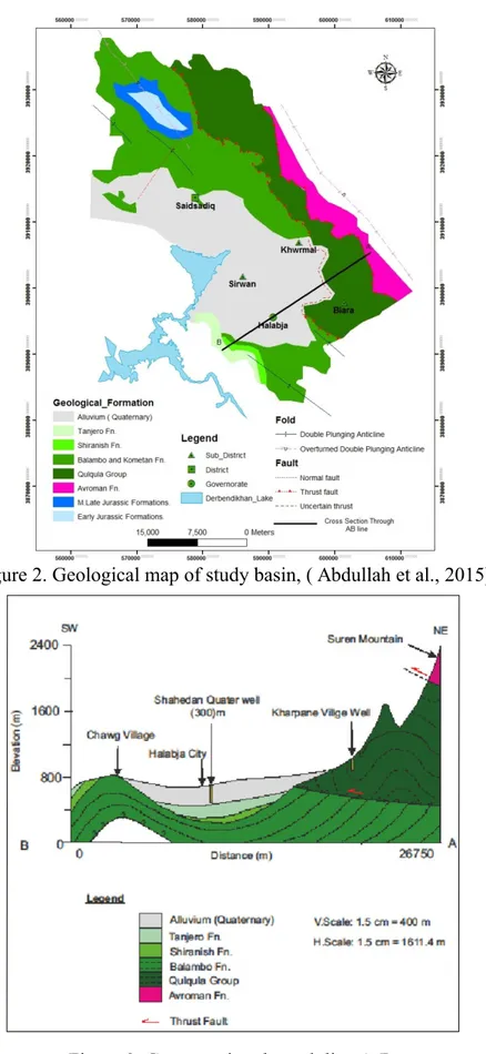
HSB is located within the Western Zagros Fold-Thrust Belt , as mentioned by (Buday, 1980, Buday and Jassim, 1987 and Jassim and Goff, 2006), structurally, is located within the High Folded zone, Imbricated, and Thrust Zones. The exposed rocks in the area are referred to the Jurassic to recent as a geological time period (Figures 2 and 3). Sarki and Sehkanian Formations of Jurassic age considered to be the oldest exposed rocks in the basin (Bellen et al., 1959). And then, followed by lower and middle Jurassic rocks including Barsarin (limestone and dolomitic limestone), Naokelekan (bituminous limestone) and Sargalu Formations, (Ali, 2007). In addition to formation of Qulqula Group had been outcropped including the Qulqula Radiolarian Formation and the Qulqula Conglomerate Formation. The exposure to the Upper Cretaceous Kometan and Lower Cretaceous Balambo Formations of (Turonian and Valanginian-Cenomanian) aging respectively, are widespread in the area where they are exposed to both sub-basins. Shiranish Formation (Campanian) and Tanjero Formation (Campanian-Maastrichtian) are also exposed in the basin but with limited outcrops.

In terms of hydrogeological characteristics and water supply , Alluvial ( Quaternary) deposits are the most important unit in the area. These sediments as mentioned by (Ali, 2007), are deposited as debris flow on the gently slopping plains or as channel deposits or as channel margin deposits and over bank

Figure 1. Location map of study basin.

deposits. The thickness of this deposit as recorded during the field observation in this study of about 300 m thick while the previous studies (e.g. Ali, 2007, Baziany, 2006, Baziany and Karim, 2007) stated that the thickness of these deposits are recorded up to 150 m thick .

Hydrogeology and hydrology of the study basin

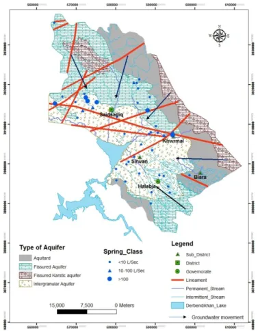
Two factor controlling the potential for the area to be considered as a water bearing aquifer, which are permeability and porosity. Several hydrogeological aquifers can be found in HSB based on different geological rock units. Types of aquifers are tabulated in Table 1. In terms of depth of the water table, from the collected data in the field and from the archives of the Groundwater Directorate at Sulaimaniyah, the mountain series, which surround the basin in the northeast and southeast, are characterized by high depth of groundwater. While toward the southeastern and the center parts, the groundwater level has a relatively lower depth. The groundwater movement is from the north and northeast and south and southeast towards southwest or generally toward the reservoir of Derbandikhan Dam (Figure 4). Hydrologically, several rivers exist on the area, such as Sirwan, Zalm, Chaqan, Biara, Reshen and Zmkan. All these rivers impound their water in Derbandikhan reservoir (Abdullah et al., 2015). There are many springs of different discharge rate present in HSB, (Figure 4). The first group having discharge that is less than 10 L/S (such as Anab, Basak, Bawakochak and 30 other springs springs). The second group having discharge of 10 to100 L/S (such as Sheramar, Qwmash , Khwrmal and Kani Saraw) and finally those have water discharge more than 100 L/S (such as Garaw, Ganjan, Reshen, Sarawy Swbhan Agha and 3 other springs)(Figure 4), (Abdullah et al., 2015). The regional lineaments as recommended by (Stevanovic and Markovic, 2004) in HSB are showed on the Figure 4.

Figure 2. Geological map of study basin, ( Abdullah et al., 2015)

METHODOLOGY

A sum of 39 groundwater samples (30 water wells and 9 from springs water) was collected at HSB during dry season (September 2014) and wet season (May 2015). The water samples were collected after 10 minutes of pumping the well in a clear pre-sterilized polythene bottles. Electrical conductivity for the collected samples was measured in the field immediately after sampling. The sample bottle were labeled, sealed, and transported to the laboratory under standard preservation methods. The major anionic and cationic concentrations were determined in the laboratory. The accuracy of the chemicalanalyses was checked using two methods, the accuracy (systematic error) of the chemical analysis for major ions can be estimated at the Electroneutrality condition and the Precision (Random error) of chemical analysis .

Based on the physico-chemical analyses, irrigation quality parameters like sodium absorption ratio (SAR), electrical conductivity (EC), sodium (Na+), chloride (Cl-) and bicarbonate (HCO3-) were calculated based on the standard quality measurement (qi) and weight for IWQI parameters proposed by (Meireles et al., 2010).Water quality maps were generated based on the calculated quality measurement multiplied by the recommended weight of each parameter using IDW interpolation technique in GIS spatial analysis. Consequently, the final irrigation water quality map was constructed by overlying of the thematic maps of above mentioned parameters and then reclassified it according to the recommended characteristics of IWQI by Meireles et al. (2010).

Uncertainty measurement of chemical analysis

Every measurement is subject to an element of uncertainty, which may be condensed by improving the method or re-analysing but can never be entirely eliminated. This uncertainty consists of two contributions: systematic error (accuracy) and random error (precision) (Gill, 1997; Appelo and Postma,1999; Rao, 2006).

Accuracy (systematic error) of chemical analysis

The accuracy (systematic error) of the chemical analysis for major ions can be estimated at the Electroneutrality condition, this is done by taking the relationship between the total cations (Ca2+_{, Mg}2+_,

Na+_{, and K}+_{) and the total anions (SO4}-2_{, HCO3}− _{and Cl}−_{) for each set of complete analyses of water}

sample (Mathhess 1982; Domenico and Schwartz 1990) using the following equation:

EN% =

∑

∑

∑

_∑

where EN% (electroneutrality) is the error percent/reaction error and Σ is the total cations and total anions expressed in milliequivalents per liter. The accepted limit or certain limit is between 0–5 %, while 5–10 % should be carefully dealt with or probable certain and > 10 % (uncertain) which is not useful for geochemical interpretation and must eliminated from the subsequent analyses.

Precision (random error) of chemical analysis

Random error of chemical analysis is the precision of a measurement is readily determined by comparing data onto carefully replicated experiments under the same conditions. The term precision is used in describing the agreement with a set of results among themselves (Al–Manmi, 2002). Precision

Figure 4. Hydrogeological map of study basin, ( Abdullah, 2015)

is usually expressed in terms of the standard deviation obtained from replicating measurements, the smaller the standard deviation, the more precise the analysis. As explained by Stoodly in (1980), precision or "Coefficient of Variation" which represents standard deviation from a group data comparing with mean %. So to calculate precision percentages, the following equation has been used:

CV(Precision)% = 2 SD

´X X 100 (2)

The accepted limit or certain limit (95 % confidence ) according to (Maxwell, 1968 )is between (5–25 %).

Table 1. Type of aquifers in the study basin.

Aquifer type Geological formation Thickness (m) References

Intergranular Aquifer Quaternary deposits more than 300 Authors Fissured Aquifer Balambo

Kometan 250 Ali,2007 Fissured-Karstic Aquifer Avroman Jurassic formation 200 From 80 to 200 Jassim and Goff,2006 Non-Aquifer (Aquitard) Qulqula

Shiranish Tanjero more than 500 225 2000 Jassim and Goff,2006

Water quality evaluation model

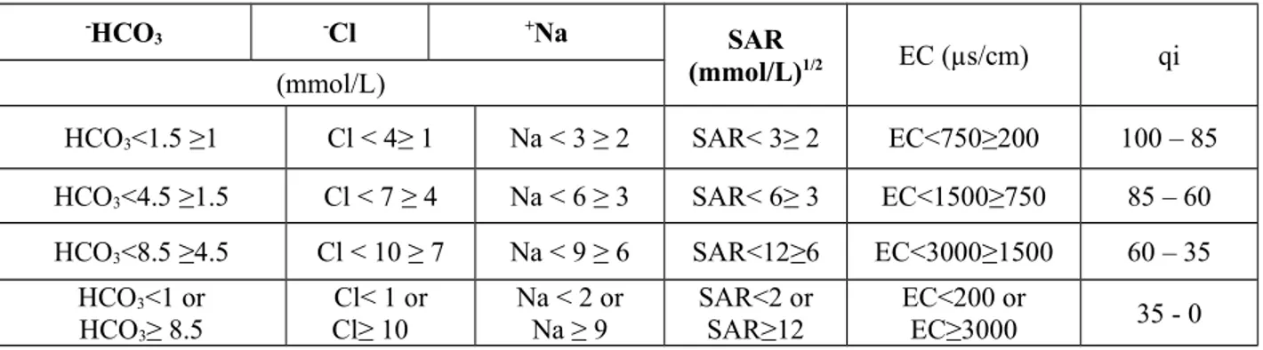
The water quality evaluation models applied to this study in two steps .In the first step, a water quality indexes WQI model was proposed. A designation of quality measurement values (Qi) and aggregation weights (Wi) were recognized. Values of (Qi) were estimated based on each parameter value shown in (Table 2) which is recommended by Ayers and Westcot (1999). Water quality parameters were symbolized by a non-dimensional number;the higher the value, the better the water quality.

Values of Qi were computed using the following equation, based on the laboratory result of water quality analysis and the tolerance limits shown in Table 2.

Qi=qimax -[

(Xij−Xinf ) x2

Xamp qiamp (3)

where qimax is the maximum value of qi for the class, Xij is the observed value for the parameter, Xinf is

the corresponding value to the lower limit of the class to which the parameter belongs; qiamp is the class

amplitude; Xamp is the class amplitude to which the parameter belongs. In order to evaluate Xamp of the

last class of each parameter, the upper limit were considered to be the highest value determined in the physical-chemical and chemical analysis of the water samples.

The weight of each parameter used in the IWQI explained on (Table 3) which is recommended by (Meireles et al., 2010) .The aggregation weights (Wi) were normalized such that their sum equals one.

Irrigation Water Quality Index Map

By summation of both Qi and Wi , the Irrigation Water Quality Index (IWQI) was calculated as

(Hussain et al. ,2014): IWQI=

∑

i=1 n

qi∗Wi ₍₄₎

IWQI is dimensional parameters ranging from 0 to 100; qi is the quality of the ith _{parameter, a}

number from 0 to 100, function of its concentration or measurement; wi is the normalized weight of the ith _{parameter, function of importance in explaining the global variability in water quality.}

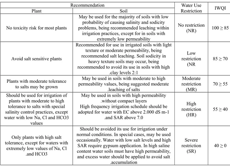
Classes division according to the proposed water quality index was based on existent water quality indexes, and classes were defined considering the risk of salinity problems, soil water infiltration reduction, in addition to toxicity to plants as observed in the classification presented by (Bernardo, 1995) and (Holanda and Amorim, 1997). Restriction to water to use classes was characterized and explained on Table 4.

RESULTS AND DISCUSSION

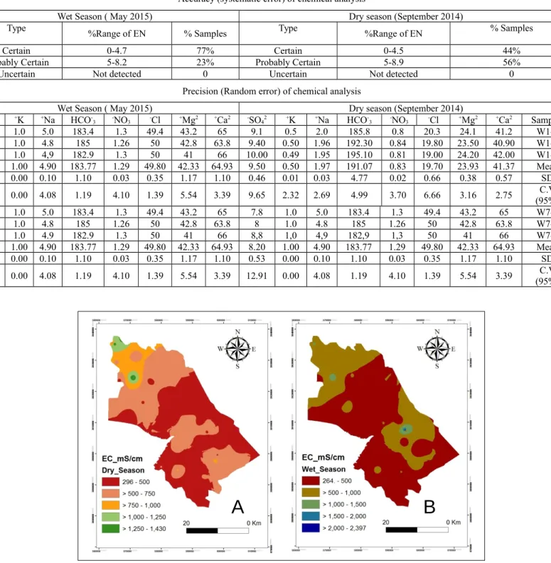
The result of uncertainty measurement of chemical analysis tabulated and explained on (Table 5). The result of both applied method within both season samples, indicates reliable analytical results and all samples of the accepted limit and should be useful for geochemical interpretation.

Table 2. Parameter limiting values for quality measurement (qi) calculation (Meireles et al., 2010) qi EC (µs/cm) SAR (mmol/L)1/2 Na + Cl -HCO3 -) mmol/L ( 85 – 100 200 ≥ EC<750 2 ≥ SAR< 3 2 ≥ Na < 3 1 ≥ Cl < 4 1 ≥ HCO3<1.5 60 – 85 750 ≥ EC<1500 3 ≥ SAR< 6 3 ≥ Na < 6 4 ≥ Cl < 7 1.5 ≥ HCO3<4.5 35 – 60 1500 ≥ EC<3000 6 ≥ SAR<12 6 ≥ Na < 9 7 ≥ Cl < 10 4.5 ≥ HCO3<8.5 0 - 35 EC<200 or EC≥3000 SAR<2 or SAR≥12 Na < 2 or Na ≥ 9 Cl< 1 or Cl≥ 10 HCO3<1 or HCO3≥ 8.5

Table 3. Weights for the IWQI parameters (Meireles et al., 2010)

Parameters

Wi

Electrical Conductivity (EC) 0.211 Sodium (Na+₎ 0.204 Chloride (Cl-₎ 0.194 Bicarbonate (HCO3-₎ 0.202

Sodium Adsorption Ratio (SAR) 0.189

Total 1.00

Chemical-Physical analysis Thematic Maps

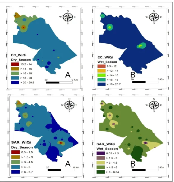
All required physico-chemical parameters required for evaluating groundwater suitability for irrigation purpose of both seasons plotted as thematic maps. Electrical conductivity is usually used for indicating the total concentration of the ionized constituents of natural water. It is intimately related to sum of the cations or anions observed from chemical analysis, and it associates affectionately with the values of dissolved solids. Electrical conductivity (EC), Figure (5) ranges of 296 and 1430 µS/cm for dry season and 264 to2397 µS/cm for wet season, with a mean EC value of (556 and 505) µS/cm for dry and wet season respectively.

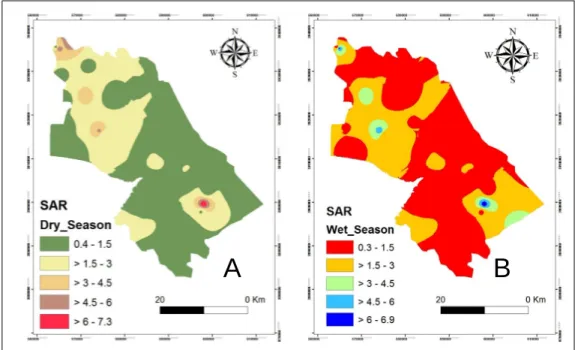
The most ordinary chemical factor that controls the normal rate of infiltration of water (infiltration

hazard) is the relative concentrations of calcium, sodium and magnesium ions in water that is also

known adsorption ratio (SAR). The Sodium Adsorption Ratio (SAR) presented on Figure (6), SAR varies from 0.4 to 7.3 with a mean value of 1.56 for dry season and 0.3 to 6.9 with mean value of 1.55 for wet season.

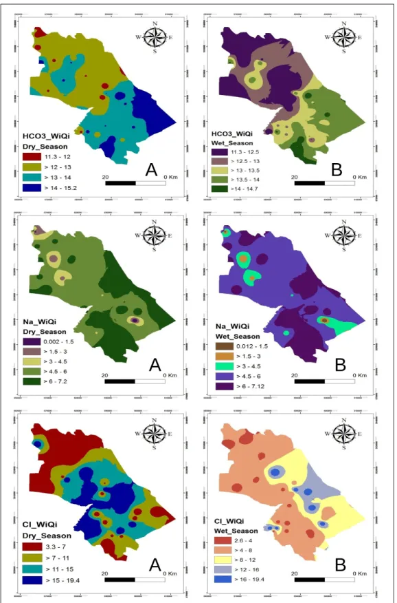
Miscellaneous Effects represented by the bicarbonates ion (HCO-_{3) which is the predominant anion}

in the both seasons samples. Ranging from 180.5 to 312.5 ppm and 182.1 to 314.2 for dry and wet season respectively (Figure 7).

The most ordinary chemical factor that controls the normal rate of infiltration of water (infiltration

hazard) is the relative concentrations of calcium, sodium and magnesium ions in water that is also

known adsorption ratio (SAR). The Sodium Adsorption Ratio (SAR) presented on Figure (6), SAR varies from 0.4 to 7.3 with a mean value of 1.56 for dry season and 0.3 to 6.9 with mean value of 1.55 for wet season.

Table 4. Irrigation Water Quality Index Characteristics (Meireles et al, 2010) IWQI Water Use Restriction Recommendation Soil Plant 85 ≥ 100 No restriction (NR) May be used for the majority of soils with low

probability of causing salinity and sodicity problems, being recommended leaching within

irrigation practices, except for in soils with extremely low permeability No toxicity risk for most plants

70 ≥ 85 Low restriction (NR Recommended for use in irrigated soils with light

texture or moderate permeability, being recommended salt leaching. Soil sodicity in

heavy texture soils may occur, being recommended to avoid its use in soils with high

clay levels 2:1 .

Avoid salt sensitive plants

55 ≥ 70 Moderate restriction (MR) May be used in soils with moderate to high

permeability values, being suggested moderate leaching of salts

. Plants with moderate tolerance

to salts may be grown

40 ≥ 55 High restriction (HR) May be used in soils with high permeability

without compact layers .

High frequency irrigation schedule should be adopted for water with EC above 2.000 dS m-1

and SAR above 7.0 .

Should be used for irrigation of plants with moderate to high tolerance to salts with special salinity control practices, except water with low Na, Cl and HCO3

values 0 ≥ 40 Severe restriction (SR) Should be avoided its use for irrigation under

normal conditions. In special cases, may be used occasionally. Water with low salt levels and high SAR require gypsum application. In high saline content water soils must have high permeability, and excess water should be applied to avoid salt

accumulation .

Only plants with high salt tolerance, except for waters with

extremely low values of Na, Cl and HCO3

.

Miscellaneous Effects represented by the bicarbonates ion (HCO-_{3) which is the predominant anion}

in the both seasons samples. Ranging from 180.5 to 312.5 ppm and 182.1 to 314.2 for dry and wet season respectively (Figure 7).

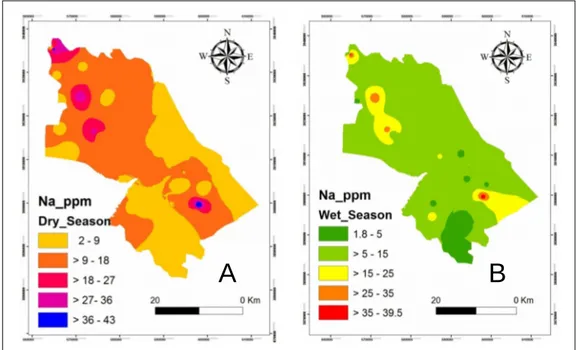
The sodium ion (Na+) concentration, is a parameter that describes the specific ion toxicity of water samples, ranged between (2 to 43 ) ppm with mean (11.16ppm) in dry season and between (1.8 to 39.5) ppm with mean (10.10 ppm) in wet season. The spatial distribution ionic concentration of sodium in HSB is publicized in Figure (8) for both seasons.

In addition chloride concentrations (Cl-_{) is also presented as the other parameter defining the}

specific ion toxicity. The chemical analysis of groundwater showed that the minimum, maximum and mean values are (17.3, 49.4 and 33.91) ppm for dry season and (14.2, 45.3 and 29.1) ppm for wet season respectively. The thematic map of chloride ion concentrations is shown in Figure (9).

Quality and weight calculation model

In order to develop the applied IWQI, several parameters were used including EC, Cl, Na, HCO3 and SAR. The weight (Wi) of each parameter was used based on (Table 3). The quality measurement (Qi) which was calculated based on Equation 1.The result of both quality measurement and applied weight presented on table (6) and Figures (10 and 11).

Table 5. Accuracy and precision calculation for chemical analysis in both seasons.

Accuracy (systematic error) of chemical analysis

Dry season (September 2014) Wet Season ( May 2015)

Samples % Range of EN % Type Samples % Range of EN % Type 44% 0-4.5 Certain 77% 0-4.7 Certain 56% 5-8.9 Probably Certain 23% 5-8.2 Probably Certain 0 Not detected Uncertain 0 Not detected Uncertain

Precision (Random error) of chemical analysis

Dry season (September 2014) Wet Season ( May 2015)

Samples Ca2 + Mg2 + Cl -NO3 -HCO -3 Na + K + SO42 -Ca2 + Mg2 + Cl -NO3 -HCO -3 Na + K + SO42 -W1-1 41.2 24.1 20.3 0.8 185.8 2.0 0.5 9.1 65 43.2 49.4 1.3 183.4 5.0 1.0 7.8 W1-2 40.90 23.50 19.80 0.84 192.30 1.96 0.50 9.40 63.8 42.8 50 1.26 185 4.8 1.0 8 W1-3 42.00 24.20 19.00 0.81 195.10 1.95 0.49 10.00 66 41 50 1.3 182.9 4,9 1.0 8.8 Mean 41.37 23.93 19.70 0.83 191.07 1.97 0.50 9.50 64.93 42.33 49.80 1.29 183.77 4.90 1.00 8.20 SD 0.57 0.38 0.66 0.02 4.77 0.03 0.01 0.46 1.10 1.17 0.35 0.03 1.10 0.10 0.00 0.53 C.V (95%) 2.75 3.16 6.66 3.70 4.99 2.69 2.32 9.65 3.39 5.54 1.39 4.10 1.19 4.08 0.00 12.91 W7-1 65 43.2 49.4 1.3 183.4 5.0 1.0 7.8 65 43.2 49.4 1.3 183.4 5.0 1.0 7.8 W7-2 63.8 42.8 50 1.26 185 4.8 1.0 8 63.8 42.8 50 1.26 185 4.8 1.0 8 W7-3 66 41 50 1,3 182,9 4,9 1,0 8,8 66 41 50 1.3 182.9 4.9 1.0 8.8 Mean 64.93 42.33 49.80 1.29 183.77 4.90 1.00 8.20 64.93 42.33 49.80 1.29 183.77 4.90 1.00 8.20 SD 1.10 1.17 0.35 0.03 1.10 0.10 0.00 0.53 1.10 1.17 0.35 0.03 1.10 0.10 0.00 0.53 C.V (95%) 3.39 5.54 1.39 4.10 1.19 4.08 0.00 12.91 3.39 5.54 1.39 4.10 1.19 4.08 0.00 12.91

Figure 5. Spatial distribution for the concentration of EC in A- dry season ,B-wet season.

Figure 6. Spatial distribution for SAR in A- Dry season ,B-Wet season.

Figure 7. Spatial distribution for the concentration of HCO-_{3 in A- Dry season, B-Wet season.}

A

B

Figure 8. Spatial distribution for the concentration of Na+ _{in A- Dry season, B-Wet season.}

Figure 9. Spatial distribution for the concentration of Cl- _{in A- Dry season , B-Wet season.}

Table 6. Weight and quality range for IWQI parameters

Parameters Dry season Wet season Wi Qi-Range Wi Qi-Range EC 0.211 62.3-97.4 0.211 45-98.3 SAR 0.189 0.1-35 0.189 0.22-35 HCO -3 0.202 56.1-72.8 0.202 55.9-72.6 Na+ _{0.204 0-35.0 0.204 0.06-35} Cl- _{0.194 16.8-100 0.194 13.4-99.8}

A

B

A

B

Figure 10. Spatial distribution for the IWQI concentration of (EC and SAR) in dry season and wet season.

The Irrigation Water Quality Index (IWQI) maps was produced according to the equation (4). The spatial analysis tool of GIS environment was used for overlapping of the thematic maps for the parameters used in this model (EC, Na+, Cl-, HCO-3 and SAR). Figure (12) illustrates spatial distribution of IWQI in HSB. According to these Figures, the area divided into three different ranges of groundwater quality of both seasons, which are (33.1-40, >40-55 and >55-66.9) in dry season and (33.42-40, >40-55 and >55-66.9) in wet season.

Irrigation Water Quality Index (IWQI) Map

The Irrigation Water Quality Index (IWQI) maps was produced according to the Equation (4). The spatial analysis tool of GIS environment was used for overlapping of the thematic maps for the parameters used in this model (EC, Na+, Cl-, HCO-3 and SAR). Figure 12 illustrates spatial distribution of IWQI in HSB. According to these Figures, the area divided into three different ranges of groundwater quality of both seasons, which are (33.1-40, >40-55 and >55-66.9) in dry season and (33.42-40, >40-55 and >55-66.9) in wet season.

A

B

Figure 11. Spatial distribution for the IWQI concentration of (HCO-3, Na+ _{and Cl}-_{) in dry season and}

wetseason.

A

B

A

B

Figure 12. Spatial distribution of IWQI map in HSB in dry and wet seasons.

Consequently, the spatial distribution of IWQI was reclassified based on ranges of water characteristics given by (Meireles et al, 2010). The suitability classes are elucidated in the Figure (13). Three classes have been recognized at HSB within both seasons. The high restriction (HR) classes to occupy an area of (52.4%) of whole HSB area in dry season and (83.3%) in wet seasons. While Sever Restriction (SR) and Moderate Restriction (MR) occupy an area of (1.4%and 46.2%) and (0.7%and 16%) for dry and wet seasons respectively. The result illustrates considerable variations materialized between SR. HR and MR and from dry to wet seasons, HR increased dramatically in wet season and MR and SR decreased significantly as well in wet season. This is due to decreasing the IWQI value of wet season as a result of dilution of water or aquifer recharge from rainfall and decreasing the water discharge from wells.

Validation of IWQI Map

The IWQI map should be validating after constructing in order to assess the validity of the theoretical sympathetic of current hydrogeological conditions. Initially, the achieved data onto laboratory chemical analysis have been assessed by measuring the uncertainty condition using two methods. The Accuracy (systematic error) and the precision (random error), the result of both methods confirmed that all chemical analysis values of each parameter used in this model is of certain and probably certain classes (Table 5) and can be useful in the geochemical analysis.

In addition, to check the attained classes of groundwater suitability for irrigation purpose by the applied model, the relation between aquifer recharges and IWQI classes have been assessed. For this reasons, fourteen wells have been selected in both dry and wet season to measure the depth to water table or Static Water Level (SWL), (Figure 14). The result of fluctuating water level of each well tabulated in Table 7, the IWQI value decreased as the water level rose up as a result of recharging from the precipitation. This outcome confirms that as the aquifer recharged, the concentration of chemical components decreased and thus confirm the validity of the applied model.

Figure 13. Reclassified IWQI map in HSB in dry and wet seasons.

Figure 14. Site of measuring SWL with reclassified IWQI map in HSB in dry and wet seasons.

CONCLUSION

The IWQI models applied to GIS environment to assess and draw the suitability of groundwater for irrigation purpose of HSB. Spatial analysis tool was used to interpolate and prepared the thematic maps of parameters applied to groundwater quality assessment such as (EC, Na, Cl, HCO3 and SAR). Based on the spatial distribution of IWQI, groundwater at HSB classified into three groups of both dry and wet seasons included; Sever Restriction (SR), High Restriction (HR) and Moderate Restriction (MR). The coverage area of all three classes is (1.4%, 52.4% and46.2%) for dry season and (0.7%, 83.3% and16%) for wet seasons respectively (Table 8). Considerable variations have been noted between HR,

A

B

MR and SR from dry to wet seasons, HR increased dramatically in wet season and conversely MR and SR decreased. Increasing aquifer recharges and decreasing aquifer discharge is the main reasons for decreasing the IWQI value of wet season. The applied model has been validated based on the relation between the aquifer recharge and spatial distribution of IWQI .As the aquifer was being recharged, the chemical elements in the water samples were decreased from its concentration and then leads to reduction in its IWQI value.

Table 7. Water level at each IWQI class in dry and wet season.

Well Dry Season Wet Season SWL(m) IWQI Class SWL(m) IWQI Class 1 61 65 MR 55 50 HR 2 60.9 66 MR 54 66 MR 3 5.65 55.5 MR 1 55 HR 4 14 60 MR 9 50 HR 5 3.5 55.8 MR 0,5 57 MR 6 26.2 57 MR 22 55.8 MR 7 10 62 MR 6 53 HR 8 20.8 57 MR 16 51 HR 9 20 57 MR 15,2 50 HR 10 64 54 HR 57,7 52 HR 11 58 58 MR 53 53 HR 12 57,3 54.8 HR 50,7 51 HR 13 38 54.8 HR 30 51 HR 14 61 53.5 HR 56,7 51 HR

Table 8. IWQI classes’ coverage area.

IWQI class Dry Season Wet Season Area % Area % Severe Restriction (SR) 1.4 0.7 Moderate Restriction (MR) 46.2 16 High Restriction (HR) 52.4 83.3

ACKNOWLEDGMENTS

The authors would like to thank Professors R. Alkhaddar of Liverpool JM University and M. Alshawi of Salford University and Kadhum Almuqdadi of the Arab Academy in Denmark for their fruitful suggestions and discussions.

REFERENCES

Ayres, R.S. and D.W. Westcot (1999). “Water Quality for Agriculture”, Irrigation and Drainage Paper No. 29, Food and Agriculture Organization of the United Nations. Rome, 1-117.

Appelo, C.A.J. and Postma, D., (1999): Geochemistry. Groundwater and pollution. Rotterdam: A. A. Balkama, 536 P.

Al-Manmi D. A. M., (2002): Chemical and environmental study of groundwater in Sulaimanyia city and its outskirts unpublished Msc. Thesis, University of Baghdad (In Arabic)

Arsalan, M.H. (2004). A GIS Appraisal of Heavy Metals Concentration in Soil; Technical Report for American Society of Civil Engineers: New York, NY, USA, 2004.

Ali S. S. (2007). Geology and hydrogeology of Sharazoor - Piramagroon basin in Sulaimani area, northeastern Iraq. Unpublished PhD thesis, Faculty of Mining and Geology, University of Belgrade, Serbia. 317P.

Alcamo, J., Florke, M., & Marker, M. (2007). Future long-term changes in global water resources driven by socio- economic and climatic changes. Hydrological Sciences Journal, 52(2), 247–275. Abdullah T. O. , Ali S.S., Al-Ansari N.A. and Knutsson S. (2015). Effect of agricultural avtivities on

groundwater vulnerability: Case study of Halabja Saidsadiq Basin, Iraq. Journal of Environmental Hydrology 23(10).The open access electronic journal found at http://www.hydroweb.com/protect/pubs/jeh/jeh2015/AnsariGW.pdf

Bellen R.C., Dunnington H.V., Wetzel R., and Morton D. (1959). Lexique Stratigraphique International. Asie, Iraq. Vol. 3C, 10a, 333p.

Buday T.( 1980). Regional Geology of Iraq: Vol. 1, Stratigraphy, I.I. Kassab and S.Z. Jassim (Eds) D. G. Geological Survey. Mining Investigation Publication. 445p.

Buday T., and Jassim S.(1987) The Regional geology of Iraq: Tectonis, Magmatism, and metamorphism. I.I. Kassab and M.J. Abbas (Eds), Baghdad, 445 p.

Bernardo, S. 1995. “Manual de Irrigação”, 4th edition, Vicosa: UFV, 488p.

Baziany M.M.Q.(2006). Stratigraphy and sedimentology of former Qulqula Conglomerate Formation, Kurdistan region, NE- Iraq. Msc thesis, Sulaimani University, 98p.

Baziany M.M.Q. and Karim K. H. (2007). A new concept for the origin of accumulated conglomerates, previously known as Qulqula Conglomerate Formation at Avroman- Halabja area, NE-Iraq., Iraqi Bulletin of Geology and Mining, Vol.3, No.2, 33-41.

Babiker, I. S., Mohamed M. M. A., and T. Hiyama (2007). “Assessing groundwater quality using GIS”, Water Resources Management, 21, 699–715.

Castellanos J.Z., Ortega Guerrero A, Grajeda OA, Va ´zquez Alarco ´n A, Villalobos S, Mun ˜o ´z Ramos JJ, Zamudio B, Martınez JG, Hurtado B, Vargas P, Enrı ´quez SA (2002) Changes in the

quality of groundwater for agricultural use in Guanajuato. Terra Latinoamenricana, 20(2):161–170. ISSN 0187-5779.

Domenico, P. A., & Schwartz, F. W. (1990). Physical and chemical hydrogeology (pp. 410–420). New York: Wiley.

Don, C.M., (1955). “A grows guide to water quality”, University college station, Texas.

Ferry, L. T., Akihiko and M. A. Mohammed Aslam (2003). “A conceptual database design for hydrology using GIS”, In the proceedings of Asia Pacific association of hydrology and water resources, Japan, Kyoto.

Gill, R., (1997). Modern analytical geochemistry, an introduction to quantitative chemical analysis for earth, environmental and materials scientists. Longman, London, 329 p.

Groundwater Directorate in Sulaimaniyah,(2014).Archive Department.

Holanda, J. S. and Amorim, J. A. 1997. "Management and control salinity and irrigated agriculture water"In: Congresso Brasileiro de Engenharia setting, 26, Campina Grande, pp.137-169.

Hiniker, M. (1999). “Sustainable Solutions to Water Conflicts in the Jordan Valley”,Cambridge Review of International Affairs, 122, 255-273.

Huang T, Pang Z, Edmunds W. (2012). Soil profile evolution following land-use change: Implications for groundwater quantity and quality. Hydrol. Process 27(8):1238-1252.

Hussain H.M.,Al-Haidarey M.J.S.M., Al-Ansari N. And Knutsson S. (2014). Evaluation and mapping groundwater suitability for irrigation using GIS in Najaf Governorate, IRAQ. Journal of Environmental Hydrology .Volume 22(4):1238-1252.

Jassim S.Z. and Guff J.C. (2006) Geology of Iraq. Jassim (Eds) D. G. Geo Survey. Min. Invest. Publication. 340p.

Khan, F., Husain T., and Lumb A., (2003). Water quality evolution and trend analysis in selected watersheds of the Atlantic Region of Canada. Environmental monitoring and assessment, 88: 221-242.

Maxwell, J.A, (1968): Rock and mineral analysis. John Wiley and Sons, NewYork, p584. Mathhess, G. (1982). The properties of ground water (1st ed.). New York: Wiley.

Meireles, A., Andrade E. M., Chaves L., Frischkorn, H., and Crisostomo, L. A. (2010). “A new proposal of the classification of irrigation water”, Revista Ciência Agronômica, 413: 349-357. Mohammed, M.N. (2011). Quality assessment of Tigris river by using water quality index for irrigation

purpose, European Journal of Scientific Research, 571: 15-28.

Richards, L. A. (1954). “Diagnosis and Improvement of Saline and Alkali Soils”, U. S. Department of Agriculture Handbook, Vol. 60, Washington D. C., USA. p.160.

Rao , N. S., (2006): Seasonal variation of groundwater quality in apart of Guntur District , Andhra Pradesh India , Environmental Geology Vol. 49 pp .413-429.

Stoodly , K.D., Lewis , T. and Staintion ,C.L., 1980 . Applied Statistical Technique. John Wiley and Sons, London. 215 P

Sadik, A.K. and S. Barghouti. (1994) The water problems of the Arab world: Management of scarce water resources, In P.Rogers and P. Lydon eds.), Water in the Arab World. Massachusetts, USA: Harvard University Press, 4-37.

Sargaonkar, A., Deshpande. (2003), development of an overall index of pollution fo surface water based on a general classification scheme in Indian context, Environmental monitoring and assessment, 89): 43-67.

Stevanovic Z. and Markovic M.(2004).Hydrogeology of Northern Iraq, Climate, Hydrology, Geomorphology and Geology.,Vol.1,2nd _{edition, FAO.}

Statistical Directorate in Sulaimaniyah,(2014).Archive Department.

Wilcox, L. V., 1955), Classification and Use of Irrigation Waters, United States Department of Agriculture, Circular No. 696, Washington, DC., p. 16.

Yogendra, K. and Puttaiah, E.T. (2008). Determination of water quality index and suitability of an Urban waterbody in Shimong Town, Karnataka, The 12th World Lake Conference; Proceeding of Taal :342-346.

ADDRESS FOR CORRESPONDENCE Nadhir A. Al-Ansari

Department of Civil, Environmental and Natural Resources Engineering Lulea University of Technology

Lulea, Sweden