Effects of within-field and landscape factors on Dasineura brassicae in winter oilseed rape cultivations in Skåne, southern Sweden

(1)

Faculty of Landscape Architecture, Horticulture

and Crop Production Science

Effects of within-field and landscape factors

on Dasineura brassicae in winter oilseed

rape cultivations in Skåne, southern Sweden

– A field survey with a special approach to pesticide-free control

zones

Emma Johansson

Degree project • [30] hec

(2)

Effects of within-field and landscape factors on Dasineura brassicae in winter oilseed rape cultivations in Skåne, southern Sweden

– A field survey with a special approach to pesticide-free control zones Effekter av fält- och landskapsfaktorer på Dasineura brassicae i höstrapsodlingar i Skåne - En fältstudie med en särskild inriktning på bekämpningsfria zoner

Emma Johansson

Supervisor: Mattias Larsson, SLU, Department of Plant Protection Biology

Examiner: Anders TS Nilsson, SLU, Department of Biosystems and Technology

Credits: 30 hec

Project level: A2E, master’s thesis

Course Title: Independent Project in Biology, A2E Course Code: EX0856

Subject: Biology

Place of Publication: Alnarp Year of Publication: 2019 Cover Art: Emma Johansson

Online Publication: http://stud.epsilon.slu.se

Keywords:Dasineura brassicae,brassica pod midge,Ceutorhynchus obstrictus, cabbage seedpod weevil, winter oilseed rape, rapeseed crop damages, pesticide-free control zones, within-field factors, landscape factors

SLU, Swedish University of Agricultural Sciences

Faculty of Landscape Architecture, Horticulture and Crop Production Science Department of Plant Breeding

(3)

Abstract

Winter oilseed rape (Brassica napus) is the most common oilseed crop grown in the province of Skåne in southern Sweden, where this study was performed. B. napus is often associated with various insect pests. This study regards two of these; the cabbage seed weevil

(Ceutorhynchus obstrictus) and the brassica pod midge (Dasineura brassicae). While direct infestations by C. obstrictus usually do not pose a major threat to B. napus cultivations, the attacks will often facilitate infestation by D. brassicae, which can cause considerable damage and subsequent yield loss through its destruction of pods. This study focuses on within-field and landscape factors that may affect abundance and damage by D. brassicae in 18 rape fields during spring and summer of 2018. Parameters investigated include chemical treatment, abundance of C. obstrictus, landscape complexity (proportion of e.g. forested areas), the proportional area of oilseed rape grown in the previous year, and distance to the nearest previous years’ oilseed rape field. Effects of chemical treatments were assessed by

establishing a pesticide-free control zone in each of the study fields. Samples were collected for nearly 10 weeks from April to July. Two field surveys of pod damages were performed during this period; the first during early pod set and the second during late pod set.

The results showed that chemical treatment had an effect on damages in early pod set. There was a progression in damage at the field edges to the field interior in early- and late pod set and in damages early in the crop season to later in the season. No relation between damages and the abundance of C. obstrictus and D. brassicae was found, nor between abundances of the study organisms. The gender ratio of D. brassicae displayed more males than females. An exceptionally warm and dry climate during the spring and summer of 2018 did have an impact on this study. The weather conditions affected the growth of the rapeseed plants and

complicated the surveys of damages. The climate may also have affected the abundances of weevils and pod midges; indeed, a considerably lower number of weevils during this season compared to the number of weevils in a study carried out during the season of 2017 was shown. Analyses of damage between regions within the province showed no significant differences between them, and landscape complexity was not correlated to abundances of the study organisms or damages by D. brassicae. Positive correlations between the proportion of rapeseed fields from the previous year and damage by D. brassicae could be reported,

however, these relationships were not consistent between damages in early- and late season or between damages at the field edge and in the inner parts of the fields. The distance to the nearest previous year's rapeseed field could not explain the abundances or damages, but a probable cause for this is the dense cultivation of rapeseed fields in Skåne.

(5)

Sammanfattning

Höstraps (Brassica napus) är den vanligaste oljeväxten som odlas i Skåne. Höstraps angrips ofta av olika skadedjur. I den här studien betraktas två av dessa; blygrå rapsvivel

(Ceutorhynchus obstrictus) och skidgallmygga (Dasineura brassicae). Angrepp av viveln utgör vanligtvis inte ett stort hot mot höstrapsodlingar, men genom sina gnaghål i

rapsskidorna möjliggör de för myggan att lägga sina ägg som senare utvecklas till små larver vilka kan orsaka betydande skador i rapsskidorna. Den här studien, som utfördes vid 18 rapsfält i Skåne under våren och sommaren 2018, fokuserar på vilka omständigheter inom fälten och i det omgivande landskapet som kan påverka förekomsten av myggor och vivlar samt skador orsakade av myggorna. Parametrar som undersökts inkluderar effekter av kemisk besprutning, fångstantal av vivlar, landskapskomplexitet (andel av exempelvis skogsklädda områden), andel vår- och höstrapsfält från 2017 års rapssäsong, och avståndet mellan rapsfälten och det närmaste höstrapsfältet från 2017 års rapssäsong. Effekter av kemisk behandling undersöktes med kontrollzoner där inga bekämpningsmedel använts. En kontrollzon per studiefält inrättades. Fällfångster av vivlar och myggor samlades in mellan april och juli under nästan 10 veckors tid. Två fältinventeringar av myggskador utfördes under fältstudieperioden; den första under rapsens tidigare skidutvecklingsstadie och den andra under det senare skidutvecklingsstadiet. Geografiska data hanterades i ett geografiskt informationssystem, ArcGIS.

Resultaten visade bland annat att kemisk behandling hade en effekt på myggskador i tidigt skidutvecklingsstadie. Inget samband mellan skador och fångstantal av vivlar och myggor hittades, inte heller mellan fångstantalet av arterna. Skidgallmyggehanarna var fler till antalet än honorna. Ett exceptionellt varmt och torrt klimat under våren och sommaren 2018 har påverkat den här studien. Väderförhållandena påverkade tillväxten av rapsplantorna och försvårade fältinventeringarna av skador. Vädret kan även ha påverkat fångstantalet av vivlar och skidgallmyggor, det faktum att ett betydligt lägre antal vivlar under den här rapssäsongen jämfört med antalet vivlar i en studie som utfördes under 2017 års rapssäsong, vittnar om detta. Inga tydliga skillnader i skador mellan olika regioner inom Skåne hittades, och undersökningar av landskapskomplexitet visade inte på samband med abundans av arterna eller skador orsakade av skidgallmygga. Positiva samband mellan andel av rapsfält från året innan och skador av skidgallmygga kunde redovisas, dessa samband var dock inte

konsekventa mellan skador i tidigt- och sent skidutvecklingsstadie eller mellan skador i fältkant och i de inre delarna av fältet. Avståndet till närmaste föregående års rapsfält kunde inte förklara antalet myggor eller skador, men en trolig orsak till det är den täta odlingen av höstraps i Skåne och därmed komplikationer i att undersöka betydelsen av avstånd.

(6)

1

1. Introduction

1.1 Oilseed rape

Oleaginous seeds, or “oilseeds”, are oil-rich seeds from which the oil can be extracted. Oilseed crops, such as soybean, rapeseed, palm kernel and cottonseed, constitutes an important part of the world grain production (Carré & Pouzet, 2014). Next after soybean, oilseed plants in the family Brassicaceae, are the worlds’ second most common oilseed crops produced, and in European agriculture these crops represent the most common (Carré & Pouzet, 2014; Zajac et al., 2016). Brassicaceae consists of species of flowering mustard- and cabbage plants where many are of great economic importance. The Brassicaceae genus Brassica contains some of the most important species, such as cauliflower and broccoli (Brassicae oleracea), turnip (Brassicae rapa) and the oilseed brassica Brassicae napus, commonly called “rapeseed”, “rape” or “oilseed rape”, hereafter “OSR” (Bañuelos, Dhillon & Banga, 2013). B. napus provides one of the world´s main source of edible vegetable oil (Unal, Sincik & Izli, 2009), which is commonly called “canola oil”. There are two distinct types of OSR, winter oilseed rape, hereafter “WOSR” (figure 1), and spring oilseed rape, hereafter “SOSR”.

OSR is an annual herbaceous plant which normally grows 1-2 meters in height (Alford, 2003). The root system is long and thin and the plants usually have several erect branches that shoot both terminally and laterally from the stem and from which small yellow flowers

develop in racemes. The foliage has a blue-green colour coated with a thin wax (Alford, 2003). The OSR fruits consist of long, narrow pods. The pods, which are green in the

immature stages and become brown as they ripen, develop from two carpels in the ovary that result in the fruit having two pod walls but which are united in the immature pods. Inside the pod, the small, black seeds develop in two rows inside two chambers (locules) separated by a rigid thin wall (septum) which parts the pod on the inside. When the pod is ripe, the united pod walls eventually split open from the base and upward, which releases the seeds but leaves the septum intact (Alford, 2003).

A B

Figure 1. The edge of a WOSR- field earlier and later in the crop season. 1(A): in early season, the photo was taken in mid-June. 1(B): in late season, the photo was taken in mid-July (photo: Emma Johansson).

(7)

2

Of the two OSR- types, WOSR is often more commonly grown as it generally has better abilities to compensate for crop damage caused by pests, diseases or abiotic factors (Alford, 2003). WOSR is sown in August to early September and harvested when the pods are ripe in summer the following year. SOSR is sown in spring and harvested in summer the same year. In order to reduce possible crop diseases, OSR is usually grown in 3-4 year crop rotations with wheat or barley after a year of fallow and with break-crops of Leguminosae variants where peas or beans are commonly grown (Alford, 2003).

In Europe, OSR cultivation has increased considerably in the past ten years (Carré & Pouzet, 2014; Weymann et al., 2015). France and Germany are the biggest growers (Carré & Pouzet, 2014; Unal, Sincik & Izli, 2009; Weymann et al., 2015) and Austria, Denmark and Sweden form another group of important producers (Carré & Pouzet, 2014). The total acres of rape and turnip rape in Sweden in 2017 was 114 800 hectares, which is an increase in production by 24% from the year before (SCB, 2017; SCB, 2018). The larger part of this consisted of rape.

OSR is mainly grown for the oil in the seeds. Products derived from OSR include cooking oil, biofuel, lubricant, cattle fodder from the plant matter, and products for the making of soaps and synthetic rubber (Alford, 2008; Williams, 2010). The most common type of OSR cultivated in Europe is the winter-type (Alford, 2003; Bañuelos, Dhillon & Banga, 2013). This is also true for Sweden, where the WOSR- cultivation have markedly expanded in the past years. Most of the WOSR in Sweden is grown in the southernmost province; Skåne, where the total production in 2017 was 168 600 tonnes, which constitutes 47% of the total production in Sweden (SCB, 2018).

Success in growth of WOSR is dependent on several factors, including the soil quality, nitrogen supply, management and the genotype (Weymann et al., 2015). Weather conditions, such as solar radiation, temperature and precipitation during specific growth stages, also constitute significant factors affecting WOSR plant development (Takashima et al., 2013; Zajac et al., 2016; Weymann et al., 2015). High temperatures and drought stress during the initial stages of pod- and seed formation have been shown to negatively affect pod

development (Angandi et al., 2000) and the maximum seed yield and oil content in seeds (Weymann et al., 2015). Drought stress during the early flowering- or seed development have also been shown to negatively affect the growth and development of WOSR plants and seeds in different ways (Bouchereau et al., 1996; Champolivier & Merrien, 1996; Hamzei & Soltani, 2012; Hatzig et al., 2018).

Apart from abiotic factors affecting WOSR growth and yield, there are also various fungal diseases (Alford, 2003, Depotter et al., 2016; Kania et al., 2018) and insect pests that occur in OSR cultivars and which may have significant impacts on production. Some examples of insect pests include the cabbage seed weevil (Ceutorhynchus obstrictus), the cabbage stem weevil (Ceutorhynchus pallidactylus), the brassica pod gall midge (Dasineura brassicae), cabbage flea beetles (Psylliodes spp.), the cabbage aphid (Brevicoryne brassicaeand) and pollen beetles (Meligethes spp.) (Alford, 2003). Only a few of these insect pests, however, pose serious threats to crop production (Alford, 2003; Vaitelyte et al., 2011).

(8)

3

This study involves two of the most important insect pests attacking WOSR in northern Europe; C. obstrictus and D. brassicae (Alford, Nilsson and Ulber 2003, Nilsson et al. 2015). While C. obstrictus may both possess the position as a primary pest and an important

aggregate for D. brassicae infestation, damage by D. brassicae is typically dependent on preceding pod invasions by C. obstrictus and usually causes greater damage in WOSR crops. The following section provides introductions to these organisms.

1.2 The study organisms

1.2.1 Ceutorhynchus obstrictus - Cabbage seed weevil

The cabbage seed weevil, Ceutorhynchus obstrictus (Marsham) (Coleoptera: Curculionidae) [syn. Ceutorhynchus assimilis Payk.], belongs to a large genus of weevils with more than 100 described species in Europe (Korotyaev, 2008) in which many prefer plant species in the family Brassicaceae for feeding and as their plant hosts for oviposition (Sivčev et al., 2015).

C. obstrictus is oligophagous on brassicaceous seed crops (Cárcamo et al., 2009) and has a

particular preference for B. napus (Gunnarsson, 2016a; Váitelyte et al., 2011). In Europe,

occurrence of C. obstrictus is especially common in regions where oilseed crops are produced (Cárcamo et al., 2009; Dosdall et al., 2002), where it has regularly become a serious pest in WOSR- crops (Cárcamo et al., 2009; Dosdall et al., 2002; Dosdall et al., 2006; Fergusson et al., 1999; Kovács et al., 2013).

Eggs of C. obstrictus are deposited into immature pods in the earliest stage of pod

development when the petals have dropped and the pistil enlargement occurs (Dosdall et al., 2002). The female pierces a hole in the pod with her proboscis where she deposits an egg (Williams, 2010). The pod is tagged with a pheromone after oviposition to inhibit repeated usage by the female herself or other females (Fergusson et al., 1999; Haye et al., 2010). Usually one egg per pod is deposited (Alford, Nilsson & Ulber, 2003), however, one single female may lay between 24 and 240 eggs in total (Williams, 2010). The eggs hatch within 1-2 weeks, after which the larvae feed on the developing seeds. The larvae undergo three larval instar stages, which span through 2-4 weeks (Dosdall et al., 2006). When the larvae are fully developed, they chew out of the pod and drop to the ground where they burrow into the soil and pupate. The new generation of imaginal adults emerges approximately 2-3 weeks later, usually in July when the pods are maturing (Dosdall & Moisey, 2004; Stephansson & Åhman, 1998). This generation of adults then feeds on the pods until the end of the crop season (Haye et al., 2010)when they migrate to nearby overwintering sites among trees, bushes, tall grass, shrubs or underneath leaf litter where they initiate the period of adult diapause (Alford, 2008; Gunnarsson, 2016a; Williams, 2010). This same generation of adults becomes active again when the soil temperature rises to 10-15ºC (Ulmer & Dosdall, 2006) and the WOSR starts to develop flowers (Alford, Nilsson & Ulber, 2003), which may happen already in the end of April (Gunnarsson, 2016b), or in late May (Ulmer & Dosdall, 2006). After emergence, the adults move to nearby WOSR- fields where they feed on the developing flower buds or the pods until it is time for mating (Alford, Nilsson & Ulber, 2003; Dosdall & Moisey, 2004). Mating occurs approximately two weeks after hibernation ends (Alford, Nilsson & Ulber,

(9)

4

2003). The life cycle of C. obstrictus generates one generation per WOSR crop season (Jordbruksverket, 2016a).

While direct infestation by C. obstrictus does not typically pose a major threat to WOSR production, the attacks will usually facilitate infestation by D. brassicae, which is a much greater problem (Aiéro et al., 2018; Jordbruksverket, 2016b; Williams, 2010). Yet,

infestations by C. obstrictus are usually controlled by the use of insecticides during the late flowering stage of the WOSR (Aiéro et al., 2018; Gunnarsson, 2016a). Some natural

regulations of populations include; larval parasitism, predation and overwintering mortality of adults (Haye et al., 2010; Williams & Cook, 2010).

A B

Figure 2. C. obstrictus. 2(A): above view (photo: Emma Johansson). 2(B): lateral view (photo: Eric Sandelin).

1.2.2 Dasineura brassicae Winn. - Brassica pod gall midge

The brassica pod gall midge (Dasineura brassicae Winn., Dipt. Cecidomyiidae), is a 0.7-2 mm sized (Stephansson & Åhman, 1998; Sylvén, 1970) dipteran which, together with C. obstrictus, belong to the most important group of insect pests of oilseed plant species in family Brassicaceae (Axelsen, 1992a). As for C. obstrictus, is B. napus also the Brassica species preferred by D. brassicae as a plant host for oviposition and development of its larvae (Åhman, 1985; Åhman, 1988).

The life cycle of D. brassicae begins in spring when the WOSR starts flowering (Graora et al., 2015). The adults emerge from the soil of fields where oilseed rape have been cultivated in the previous year (Alford, Nilsson & Ulber, 2003; Williams & Cook, 2010). Depending on the air- and soil temperature, emergence may already begin in mid-April (Graora et al., 2015), however, more commonly most gall midges appear in the end of May (Alford, Nilsson & Ulber, 2003; Stephansson & Åhman, 1998). The adult pod midges only live for 1-2 (Sylvén, 1970) or 3-5 (Isidoro et al., 1993) days, thus, the males and females may start to mate immediately at the location where they emerge. Shortly after mating the males die while the fertilized females fly to a nearby WOSR- field, navigating by vision (Murchie, Smart & Williams, 1997; Williams & Cook, 2010) and olfactory search (Molnár et al., 2018; Murchie,

(10)

5

Smart & Williams, 1997; Williams & Cook, 2010). The females oviposit eggs inside immature pods (Moser et al., 2009; Stephansson & Åhman, 1998) and die shortly after oviposition (Åhman, 1987). Pod gall midges are poor flyers. Dispersion is therefore often dependent on wind strength and direction (Williams & Cook, 2010), thus, the midges usually do not reach more than a few hundred metres from their overwintering site (Moser et al., 2009; Zaller et al., 2008b), or, occasionally they may disperse up to 1-1.5 km if the wind is weak or absent (Stephansson & Åhman, 1998). Oviposition is usually only enabled through prior pod damage caused by C. obstrictus that, as mentioned in the previous section, creates pin-sized holes in the pods for feeding and oviposition of its larva (Hughes & Evans, 2003; Murchie & Hume, 2003; Åhman, 1987). The pod midges may however penetrate the pods themselves in certain cases, such as in the case of young pods (therefore more easily

penetrated), or if the pods have been damaged due to other factors such as damages by insects other than C. obstrictus, or weather damages (Axelsen, 1992a; Nilsson, Vimarlund &

Gustafsson, 2004). The female oviposits several clusters of eggs inside one pod, and one female may use up to three pods (Stephansson & Åhman, 1998; Åhman, 1987).

The eggs develops into 1-2mm white or yellow larvae only after a few days inside the pod (Alford, Nilsson & Ulber, 2003; Pavela, Kazda & Herda, 2007; Åhman, 1985). The third instar larvae releases an enzyme on the inner wall tissue of the pods to facilitate feeding, which results in pod distortion, discolouration and eventually desiccation and cracking that causes early shedding of the seeds. Ultimately, this will result in losses in crop yield (Alford, Nilsson & Ulber, 2003; Graora et al., 2015; Jordbruksverket, 2016b). The larvae feed on the pod for approximately 2-4 weeks before the pod cracks and eventually releases the larvae that fall to the ground, burrow down in the soil and spin cocoons (Alford, Nilsson & Ulber, 2003; Graora et al., 2015; Stephansson & Åhman, 1998). The larvae may then pupate within the cocoon which can give rise to a second generation of adults approximately two weeks later. This generation will then fly to a nearby SOSR- field (Williams, 2010). The first generation larvae can also enter winter diapause within the cocoon. The diapause may last until next spring before emergence of adults, or it may even last for a few years in the case of unfavourable climatic conditions (Alford, Nilsson & Ulber, 2003; Ferguson et al., 2004; Williams, 2010; Williams & Cook, 2010). A third and fourth generation D. brassicae can also emerge, but by the time of these generations’ emergence, the cropping season will soon be over which decreases the probabilities for these females to find adequate hosts (Stephansson & Åhman, 1998). For every generation of D. brassicae, more adults enter diapause and then emerge in the following years (Hughes & Evans, 2003; Stephansson & Åhman, 1998), however, the mortality during overwintering is high (Stephansson & Åhman, 1998). The foremost important natural regulation of populations of D. brassicae is predation by hymenopteran parasitoids (Ferguson et al., 2004; Gunnarsson, 2017b).

(11)

6

1.3 D. brassicae in Sweden

Abundance of C. obstrictus and WOSR- crop damages by D. brassicae in Sweden have been relatively restricted to the field edges and thus have not been an issue of importance in the past (Aiéro et al., 2018; Jordbruksverket, 2016b; Nilsson, Vimarlund & Gustafsson, 2004). However, in the past years the situation have been different. D. brassicae damages, along with drought in some years, caused considerable losses in crop yields in Skåne in 2015-2017 (Aiéro et al., 2018; Andersson et al., 2015; Gunnarsson, 2016b; Jordbruksverket, 2016b). In 2016, for example, drought and infestations by D. brassicae resulted in a kg/ha yield loss by almost 35% from the year before in southern Sweden (Gunnarsson 2016b; SCB, 2016; SCB, 2017) and caused significant yield losses in the eastern part of central Sweden (Aiéro et al., 2018).

There are no established forecasting methods, and hence no threshold values for insecticide treatments, for specific control of D. brassicae. The pod midges often migrate to the WOSR- fields continuously for a long period during crop season which makes them particularly difficult to control (Jordbruksverket 2017; Jordbruksverket, 2016b) and the reproductive success of D. brassicae in one crop season do not seem to automatically result in a worse or similar situation in the subsequent season (Nilsson, Vimarlund & Gustafsson, 2004). Hence the abundance and damages by D. brassicae is often not frequent between years. Moreover, because the pod midges are very small and die shortly after oviposition (Stephansson & Åhman, 1998), they are very difficult to detect in field. Insecticides for specific control of D. brassicae is thus not used in Sweden (Jordbruksverket, 2016a; Jordbruksverket, 2016b; Nilsson, Vimarlund & Gustafsson, 2004), but as there are recommendations for chemical treatments for the direct control of infestations by C. obstrictus, this indirectly concern control of attacks by D. brassicae as well (Aiéro et al., 2018; Gunnarsson, 2016a).

Other methods to regulate D. brassicae apply to a landscape-level spatiotemporal rotation. To avoid diseases and pests, cultivation of WOSR is practiced in crop- rotations, hence, is not

A B C

Figure 3. 3(A): Seeds- and D.brassicae larvae inside a B. napus pod. 3(B): A female of D. brassicae (note the ovipositor). 3(C): A male of D. brassicae (photos: Emma Johansson).

(12)

7

cultivated in the same field for several consecutive years (Alford, 2003). Therefore, as the gall midges have a short adult life and cannot migrate far, predictions of abundance in one crop season may be based on the amount of closely located Brassica plant fields from previous crop seasons (Jordbruksverket, 2016b; Nilsson, Vimarlund & Gustafsson, 2004). A general recommendation is therefore to grow WOSR at safe distances to where WOSR was grown in the previous season (Stephansson & Åhman, 1998).

There are also other factors that can randomly affect the reproductive success and thus the magnitude of damages by D. brassicae in a particular season. Such factors include soil temperatures (Axelsen, 1992a; Nilsson, Vimarlund & Gustafsson, 2004), weather conditions (Nilsson, Vimarlund & Gustafsson, 2004), distances between hibernation fields and the WOSR- fields for oviposition (Jordbruksverket, 2016b; Moser et al., 2009), amount of forested land features in the neighbouring landscape (Zaller et al., 2008a), abundance of C. obstrictus (Åhman, 1987), and seasonal timing of pod development and emergence of adults (Stephansson & Åhman, 1998).

As previously mentioned, damage by D. brassicae has been a large problem in Skåne in the past three years (Aiéro et al., 2018; Andersson et al., 2015; Holmblad et al., 2017). The problem with D. brassicae in Skåne can therefore be expected to continue in the 2018 WOSR season. Presently it is not entirely known why populations of D. brassicae, and thus inflicted crop damages, increase in certain years (Gunnarsson, 2016b). However, as the climate becomes warmer and the winters become milder, the growth season of WOSR becomes longer and the acres of WOSR- cultivation expand further north (Berg, 2012). Along with these events, future prospects will possibly show that the already established problems with insect pests in WOSR- cultivation, in particularly the problems with D. brassicae, will also expand. It is therefore of relevance to obtain further knowledge about factors governing population density and severity of this pest.

1.4 Landscape factors

In extensive agricultural landscapes there will be a large number of insect pests whose life cycles are closely connected to the crops being cultivated (Alford, 2003). The ability of these insect pests to spread may increase in a fragmented landscape with expansive conventional farming systems where much of the natural vegetation has been removed since, for example, this can often result in a decline of natural predators (Bianchi, Booij & Tscharntke, 2006; Chaplin‐Kramer et al., 2011; Mazi & Dorn, 2012; Thies et al., 2011; With et al., 2002). Earlier studies have investigated the relations between abundances of insect pests and damages in crops and the distances to, - and areas of their host plants in the neighbouring landscape. Sometimes with contradictory results. As an example, Thies, Steffan-Dewenter & Tscharntke (2003) found no correlations between the total percentage of OSR in the

surrounding landscape and the abundance of pollen beetles, while Zaller et al. (2008b) found a negative correlation between the same landscape parameter and organism but a positive correlation for another OSR pest; the stem weevil. When the abundances of D. brassicae and

(13)

8

C. obstrictus and the area of OSR in the surrounding landscape were investigated in two studies, either no relationship was found for D. brassicae (Zaller et al., 2008b) or was negatively correlated for both D. brassicae and C. obstrictus (Zaller et al. 2008a). Hence, clearly there are gaps of knowledge about the relations between landscape parameters and abundances and damages by D. brassicae, but understanding more about the ecology of D. brassicae may increase the chances of avoiding crop damages by this pest in the future. This study focuses on three landscape parameters; the complexity of the landscape (proportion of e.g. forested areas) in the neighbouring landscape, the proportion of OSR- crops in the neighbouring landscape, and the distances to the closest WOSR- field from last year.

1.5 Objectives

The aim of this study is to examine how within-field and landscape factors affect and relate to pod damages caused by D. brassicae in 18 study fields with WOSR- cultivation in Skåne county, southern Sweden. A 24m x 20m zone which is free from application of chemical insecticides, in this study called a Pesticide free-control zone, hereafter “PFCZ”, has been established in each of the study fields in order to investigate the effects of use by chemical treatments on damages by D. brassicae. Issues which are considered in this study include the distribution of damages within the fields, the abundance of C. obstrictus, the area of WOSR-fields in the previous year, the distance between the closest WOSR- WOSR-fields from 2017 to the study fields, and landscape complexity. The parameters included in this study are chosen based on previous knowledge of the biology of the study organisms (see section 1.2) and based on the study by another student from last year (Rösvik, unpublished, 2017). Sex ratio of D. brassicae will also be assessed.

Study questions and hypotheses

- How does the phenology of abundances of the study organisms evolve as the crop season progresses? The hypothesis is that abundances of D. brassicae and C. obstrictus in traps will decrease later in crop season, whereas field damages will increase.

- What is the sex ratio of D. brassicae males and females determined by trap catches? Based on the notion that fertilized females migrate to WOSR-fields from the overwintering fields, it is hypothesized that more females than males will be found in the samples.

- Is the approach of in situ counting of weevils early in the crop season an applicable predictor of abundances of weevils later in the crop season and, hence, for the decision upon the use of chemical treatments in the field?

- What is the relation between abundance of D. brassicae and C. obstrictus?

- Are there any statistically significant differences in abundances of D. brassicae and C. obstrictus within- and outside of the PFCZ?

- Are there any statistically significant relationships between the abundance of C. obstrictus caught in the two trap types?

- How does abundances of C. obstrictus in the study conducted during the season of 2017 differ from abundances in this study?

(14)

9

- Damages by D. brassicae will be greater in the field border compared to 20m into the field in both early pod set(i.e. early in the crop season) and late pod set (i.e. later in crop season). - Is damages by D. brassicae greater within the PFCZ compared to the surveyed parts of the

WOSR- fields outside of the PFCZ?

- What is the relationship of damages by D. brassicae between early pod set and late pod set?

- What is the effect of abundances of C. obstrictus and D. brassicae and chemical treatments on damages by D. brassicae? It is hypothesized that damages by D. brassicae will correlate positively with the abundance of D. brassicae and C. obstrictus.

- Are there any difference in damages by D. brassicae and abundance of D. brassicae at different geographical directions within the study region?

- How does landscape factors, i.e. the proportion of forested- and grassy land types, the quantity of previous year OSR- fields, and the distance between the closest previous year WOSR- field centre points to the study fields centre points, relate to damages by D.

brassicae and abundances of D. brassicae and C. obstrictus? On the account of the biology of the study organisms (section 1.2.1 and 1.2.2), landscape complexity is thought to

correlate positively with abundance C. obstrictus and the proportion of OSR- fields from 2017 and distances between OSR fields in 2017 and 2018, is thought to correlate positively to abundance of D. brassicae or damage by D. brassicae.

Finally, a questionnaire was compiled and sent to the WOSR-growers after the crop season had ended. The questions were geared towards the management of the WOSR- cultivation and the farmers’ perceptions regarding this years’ abundances and damages of C. obstrictus and D. brassicae compared to the previous year.

2 Material and methods

All the maps presented in the report are produced in ArcGIS software (ESRI, Redlands, CA).

2.1 The study region

The study was conducted in the province of Skåne in Sweden's southernmost part (figure 4). This region is mainly characterized by arable land, which cover about 40% of the total land mass of the province (SCB, 2018). The two main crops cultivated in 2017 was Winter wheat, which covered ⁓24% of the total arable land, and spring barley that covered ⁓16%. OSR- crops constituted ⁓11% of the total arable land in Skåne in 2017, this is ⁓43% of all OSR grown in Sweden which makes Skåne the most important OSR-growing region in the country. Of the total hectares of OSR grown in Skåne in 2017, WOSR constituted 99.5% (SCB, 2018). This study was performed in the summer of 2018. The province of Skåne has a mild climate relative to other more northerly parts of Sweden. The average temperature normally ranges between 15 to 17 ºC in July and the annual precipitation ranges between 500mm and 1000mm (SMHI, 2016a).

(15)

10

2.2 The study sites

The farmers that participated in this study were contacted through phone calls. Some of them had been participating in a similar study conducted last year, and some were participating for the first time. The selection of the study localities was primarily controlled by the willingness of the participants to leave a PFCZ in their field, and this did to some extent affect the number of participants in the study and the locations of the study sites within the study region.

Ultimately 18 fields were included in the study (figure 4). The area of the fields can be viewed in the table in appendix 1.

Figure 4. Map of Skåne and the localities of the WOSR- fields. Most towns, roads, lakes and watercourses in Skåne has been excluded in the map, however, the largest cities, towns, lakes and rivers are included for orientation purposes.

2.3 Fieldwork

2.3.1 Collection of trap samples

Field work was conducted for approximately 10 weeks between 18-04-26, when the first traps were placed in field, and 18-07-10 when the last traps were collected from the field. This period covered the beginning of blooming until shortly before harvest.

To mark PFCZ at each of the study fields, a red flag was placed in each corner of the PFCZ. The flags were taller than the height of the canopy when it was fully developed in order to be easily detected by the farmer when it was time to apply insecticides.

Two yellow pan traps (donated by Dupont) and two yellow sticky traps (20 x 25cm,

(16)

11

in the middle of the field edge. One trap of each kind was placed at the field border within the PFCZ, and the other two traps were placed a few metres outside of the PFCZ. Both types of traps were attached to wooden sticks to locate the traps at a desirable height in the canopy of the WOSR- plants (figure 5, 6). The sticky traps were covered with wire netting to prevent unwanted animals (e.g. birds) from getting caught, and to prevent predation. For the same reason, the pan traps also had a net, which covered the hole of the bowl. To catch insects in the pan traps, they were filled with water and a small amount of dish washing detergent. The traps were placed in field between 18-04-26 and 18-05-11. From the date when the traps had been placed in field to the date when they were taken down, each field was visited approximately once in a week to collect the samples and renew the traps. The fields were visited in the same order as the traps had been set up. At each visit, the sticky traps were covered with cling film and marked with locality, date, and if it was collected within the PFCZ or not. After collection, a new sticky trap was positioned on the stick. The contents of the pan traps were filtered through large tea filters which were then stored in plastic tubes filled with 70% ethanol and marked in the same way as the sticky traps. All samples were kept in a fridge after each collection until they were sorted and analysed.

The quantity of individuals of the study organisms were documented in lab. A stereo microscope was used when needed for identification and counting. On the sticky traps, the number of individuals of both species were counted, however in the pan trap samples, only individuals of C. obstrictus were counted. For identification and counting of individuals of D. brassicae, a 2 x 2cm grid was charted on an overhead transparent plastic sheet which was placed on top of the sticky traps. Using this grid was crucial for a systematic browsing of the traps and to prevent double-counting and oversight of individuals. Apart from individual counts of D. brassicae, gender was documented to allow for sex ratio analyses.

The traps were present in field between 55 and 74 days throughout the field work process. The difference in number of field days was due to the rather large amount of time it took to perform the field surveys of damages by D. brassicae at each study site, which disrupted the time sequence and schedule for field visits. In order to consider this variation in number of field days in the statistical analyses, the parameter of individuals/day was used as a metric of abundances of C. obstrictus and D. brassicae instead of applying the total number of

individuals.

Figure 5. Yellow pan traps at the edge of two different WOSR- fields in the scene of late pod set. Right picture: the results of severe drought, the state of most WOSR- fields later in the crop season in this study due to the weather conditions in the summer of 2018 (photo: Emma Johansson).

Figure 6. A yellow sticky trap at the edge of a WOSR- field in late pod set. The trap is covered with wire netting (photo: Emma Johansson).

(17)

12

2.3.2 Field survey of damages by D. brassicae

Field surveys to record damages by D. brassicae were performed at two occasions. The first survey was conducted between 18-06-04 and 18-06-15, which was the period shortly after early pod formation, and the second survey was conducted between 18-07-02 and 18-07-10, which was the period of late pod formation. BBCH of the crops was 69-79 at the time of the first survey and 85+ at the time of the second survey (Lancashire et al. 1991). The basic methodology of the surveys followed a protocol by the Swedish Board of Agriculture (SBOA), however the methodology was somewhat adjusted, primarily to fit with the PFCZ- approach of this study. According to the protocol by SBOA, surveys of damages by D. brassicae are performed at two sites in each test field. At each location, a total of 20 WOSR-plants are inspected. One of the sites is located at the field edge and the other is located 20 metres into the field. The first-, the secondary-, and the main inflorescence of each WOSR-plant is inspected for damages. The percentage of damage of each WOSR-plant is then obtained by counting all the pods and all the damaged pods at each inflorescence. Below is described how the surveys in this study were performed.

In this study, the approach for the field survey of damages differed in the first and second survey due to time- and labour constraints at the time of the first survey. Four locations and a total of 40 plants were checked for pod damages in the first survey, while ten locations and a total of 100 plants were checked for damages in the second survey. The first survey included two locations situated within the PFCZ where 10 plants located at the traps at the field edge of the PFCZ and 10 plants 20m into the PFCZ, were checked for damages. The other two sites were located outside of the PFCZ. In the second survey, the same locations as those included in the first survey were also included in this survey; however, an additional six locations which were located at the remaining three sides of the field, were also included. Figure 7 shows the spatial configuration of the field surveys where each of the sample sites in the surveys represent an inspection of 10 plants.

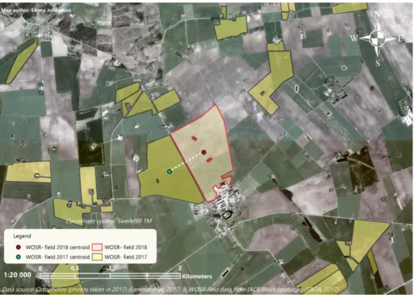
Figure 7. A WOSR- field in this study and the location of a nearby WOSR- field from 2017. The field centroid and the locations of sticky traps, pan traps, the PFCZ and D. brassicae survey sample sites, are marked. The small inserted figure shows a detailed view of the PFCZ and the traps and survey sample sites within it.

(18)

13

The final metrics of damages which was used in the statistics, was the mean percentage of damage for every B. napus plant. Non-infested pods, damaged pods and the number of bare pod stalks on the racemes on each florescence, was calculated. The number of bare pod stalks was subtracted in the calculations since such damages are likely caused by factors other than D. brassicae, such as pollen beetles (Zaller et al., 2008a).

2.3.3 Analyses of landscape factors

All data containing geographic information of the distribution of WOSR- fields from last year and ground-cover data which are included in the landscape analyses, was managed in ArcGIS (ESRI, Redlands, CA). Landscape complexity and the area of OSR- fields from 2017 was analysed within defined distances from the study fields. Four circular buffer zones with radiuses of 3000 metres, 2000 metres, 1000 metres and 500 metres were drawn around a centre point of each WOSR- field (figure 8). The sizes of the buffer zones were primarily chosen based on the current notion that D. brassicae usually do not disperse further than 0.5-1.5 km from its emergence sites (Moser et al., 2009; Stephansson & Åhman, 1998; Zaller et al., 2008b), while C. obstrictus may fly much further than 2 km from its hibernation sites (Dosdall et al., 2006; Tansey et al., 2010). Smaller buffer zones were not subtracted from the larger in the statistical analyses because usually it is not done in these types of analyses and hence to compare with previous studies it was not done in this study either.

Landscape variables used to describe the landscape complexity around the study fields included spatial information of land types in Skåne derived from the Swedish ground cover data (Svensk marktäckedata, SMD). Other landscape variables included the distances between the centre points of the closest WOSR- fields from last year and the centre points of the study fields, and the areas of OSR- fields in 2017. The SMD data, collected from the Swedish Environmental Protection Agency, consists of ground cover classes based on the European classification system CORINE land cover (Naturvårdsverket, 2014). According to this system, there can be different types (classes) of a particular land feature. For example, coniferous forest consists of six classes. In this study, the different types were reduced into a single land type- such as “coniferous forest”. Ultimately this resulted in a total of 25 classes merged into 14 land types which were finally used in the landscape analyses (table 1). The metrics of landscape complexity constituted the summed total percentage of the different land types within each of the four buffer zones around each study field.

Land type SMD code

Non-urban park 1425 Urban green-areas 141, 1426 Orchard 222 Pasture land 231 Deciduous forest 3111, 3112, 3113 Coniferous forest 31211, 312121, 312122, 3122, 3123, 31212 Mixed forest 3131, 3132, 3133 Scrub 3241 Clear-cut 3242

(19)

14 Young forest 3243 Limnogenic wetland 411 Mire 4121 River/Stream 511 Lake/Pond 5121, 5122

Data including WOSR- fields in 2017 was derived from the Integrated Administration and Control System (IACS, “Blockdatabasen”), governed by the Swedish Board of Agriculture (SBOA). IACS include annually updated crop-specific codes for all the registered agricultural fields in Sweden. Distances between the centre points of the WOSR- fields and the centre point of the closest WOSR- field from 2017, were calculated in ArcGIS (figure 9). The data was then exported to Microsoft Excel to calculate the percentage of each land type and WOSR- field within each buffer zone for all the study sites. Both winter- and spring rape fields from 2017 were implemented in the calculations as C. obstrictus and D. brassicae may also attack SOSR (Graora et al., 2015; Stephansson, 1998). The amount of SOSR- fields within the buffer zones was, however, negligible relative to the number of WOSR- fields and was often not contained within the buffer zones. Data of WOSR- fields from 2018 other than the study fields, could not be included in the calculations as this information was not

accessible at the time when these calculations were made.

A B

Figure 8. The maps show: the spatial arrangement of three of the WOSR fields included in this study, buffer zones around each WOSR field, agricultural field data (IACS), and Swedish ground cover data (SMD). 8(A): four buffer zones drawn around the centre points of three 2018 WOSR fields, the 2017 WOSR fields within the buffer zones are highlighted. 8(B): the geographic information within the buffer zones is extracted.

(20)

15

Figure 9. Ortophotos (from 2017) of the nearby landscape to one of the WOSR study fields, where the 2017 WOSR- fields are highlighted. The centre point of the study field and the centre point of the closest 2017 WOSR- field are marked. The dashed white line illustrates the distance between the fields’ centroids.

2.4 Data management and statistical tests

The statistical analyses were performed using SPSS (vers. 12.0.1 for Windows, SPSS Inc., Chicago, IL, USA). SPSS was also used to generate most graphics. Microsoft Excel was used for data compilation, calculations and some graphics. Two graphics were also generated in R (R Core Team 2018) and ggplot2 (Wickham, 2016). All datasets were tested for normal distribution according to Kolmogorov-Smirnov and Shapiro-Wilk tests of normality before statistical analyses were performed (Ghasemi & Zahediasl, 2012). If the dataset to be analysed was normally distributed, applicable tests for normally distributed data was used, and

likewise, equivalent tests for datasets which deviated from normal distribution was used if data was not normally distributed.

Mean trap catches of the study organisms throughout the period of field work were displayed with graphics computed in R statistical software and ggplot2.

Difference in abundances of D. brassicae males and females counted on the sticky traps was tested with a Mann-Whitney U-test and a Spearman rank correlation test was computed to assess the relation between males and females mean abundances.

A common way to determine if chemical treatments should be applied in the field is to look for C. obstrictus on the flower buds in situ in the earliest stage of development of the WOSR flowers, which is also the initial period of C. obstrictus immigration. Threshold values for application of chemical treatments in Sweden is 1-2 weevils/plant. To investigate if the number of counted weevils were related to the sizes of trap catches of weevils in this study, number of weevils were counted on ten plants within the PFCZ at each field visit during the

(21)

16

first four weeks of fieldwork. This was then tested with spearman rank correlation tests to assess relations with total trap catches of weevils in the pan traps and the sticky traps in the first four weeks.

The relation between abundances of D. brassicae in the sticky trap samples and the

abundances of C. obstrictus in the sticky trap- and in the pan trap samples, was examined with Spearman rank correlation tests.

Differences in abundance of C. obstrictus in the pan traps and D. brassicae and C. obstrictus in the sticky traps obtained within the PFCZ and outside of the PFCZ was tested in order to assess if chemical treatments would affect presences of individuals before they had reached the fields. Since these trap catches cannot be regarded as independent samples, the

differentiations of abundances between the traps was calculated and tested with a One- sample t-test or Wilcoxon signed rank test.

The relation between abundance of C. obstrictus in the two trap types was tested in order to evaluate the efficiency of the trap types. This was tested with a Spearman rank correlation test.

Differences in mean abundances (catch/day) of C. obstrictus in sticky trap samples and pan trap samples in the study conducted during the season of 2017 (Rösvik, 2017) and the abundances in this study, were assessed with Mann-Whitney U-tests. Damages by D.

brassicae was not compared due to considerable differences in the methodologies in the two studies and differences in abundances of D. brassicae could not be assessed because this parameter was not included in the 2017 study.

To test the differences in total mean percentage of damages by D. brassicae from within- and outside of the PFCZ at the field edge and 20m into the field in early- and late pod set, the datasets for each sample point were subtracted to obtain the differentiations in damages which was then tested with One- sample t-tests or Wilcoxon signed rank tests. To assess the

progression of total mean damages within the PFCZ and outside of the PFCZ at the field edge and 20m into the field in early- and late pod set, Pearson- or Spearman rank correlation tests were computed.

The relationship of within-field damages by D. brassicae in the field border and 20m into the field between early- and late pod set was examined with Spearman- or Pearson correlation tests.

Multiple regression models were computed to evaluate the effects of abundance of D.

brassicae in sticky traps and C. obstrictus in sticky traps and pan traps and chemical treatment on damages at the field border and 20m into the field within- and outside of the PFCZ in early- and late pod set.

Differences in damages by D. brassicae in a geographic perspective in early- and late pod set at the field border and 20m into the field, was examined using a factorial univariate analysis of variance or Kruskal-Wallis H test. The study sites were divided into five cardinal

directions; Middle, Northeast, Northwest, Southeast and Southwest, accordingly to where within the study region the sites were located (figure 10).

(22)

17

Figure 10. The map shows the categorization of the study sites into cardinal directions within the study region, Skåne. Agricultural land in Skåne is shown, other land-types are excluded.

Multiple regression models were computed to assess the relationship between abundances of C. obstrictus and D. brassicae and damages by D. brassicae within- and outside of the PFCZ at the field edge and 20m into the field against landscape complexity and hectare of OSR from 2017 within 3000, 2000, 1000 and 500 metres buffer zones. The distance to the centre point of the nearest WOSR- field from 2017 from the study fields’ centre points were also included in the models. This landscape parameter was also tested with single correlation analyses using Spearman rank or Pearson correlation tests.

3 Results

3.1 Abundances of D. brassicae and C. obstrictus throughout the crop season

A total of 3372 weevils and 8015 pod midges were caught during the field study, where 794 of the weevils were caught in the sticky straps and 2578 weevils were caught in the pan traps. Figure 11 shows the mean trap catches of D. brassicae and C. obstrictus per day with a trend line and ±95% confidence intervals throughout 2.5 months, which cover the whole period of field work. There were large, and sometimes extreme, variances in trap catches between the samples. The data in these figures is thus shown in Log10 to fit all samples in order to display complete trends in the phenology of the species. The set-up of traps at the fields in the

beginning of this study was, as explained earlier, not performed during one single day. This occurred between 18-04-26 and 18-05-11. Since the fields were visited once a week from the day the traps had been located in field, the dates for the field visits do not appear in a strict

(23)

18

chronological order. The date intervals thus represents one emptying round at each field, which results in overlaps of the dates in figure 11.

A

B

Figure 11. Box plots showing mean abundance of 11(A) D. brassicae and 11(B) C. obstrictus and trend lines adjusted to the data and with ±95% confidence interval. The x-axis shows general dates for the field visits and the legends displays the specific dates and the total number of samples for each visit. The figures are created in R statistical software (R Core Team 2018) using ggplot2 statistical software (Wickham, 2016).

3.2 Difference in, and relation of, abundance of D. brassicae male and female

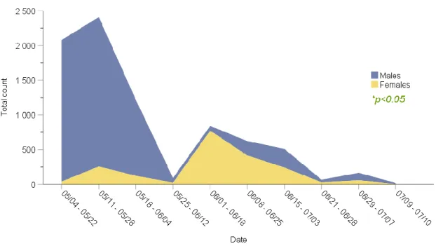
A total of 8015 D. brassicae midges were counted on the sticky traps. Of these, 6066 were males and 1957 were females, giving the proportion male as ⁓0.76. Figure 12 shows the trend of abundance of males and females over the period of fieldwork. The date intervals overlap because of the same reason already explained in section 3.1.

The test results showed a statistically significant difference in abundances per day of D. brassicae males and females, where mean abundance of males was larger (U=82, n=36, p<0.05, mean/daymales=2.66, mean/dayfemales=0.88), large outliers were not excluded in this test (figure 13). Differences in male and female abundances were also tested with the outliers excluded. This dataset was still not normally distributed and did also show a statistically significant difference between abundances of males and females (U=66, n=33, p<0.05,

(24)

19

mean/daymales_{=1.1, mean/day}females_{=0.38). A positive correlation was found between males}

and females mean abundances per day (r=0.562, n=18, p<0.05) when the outliers were not excluded (figure 13). The relation between male and female abundances were also tested with the outliers excluded, and this did not show a statistically significant relation between male and female abundances (r=0.414, n=18, p>0.05).

Figure 12. Total abundance of males and females throughout the crop season. Both male- and female data is displayed staring from 0 on the y-axis The x- axis shows the time period for each of the ten visits to the fields during the period of fieldwork. The date-periods overlap due to the differences in dates when the traps were located in field.

A B

Figure 13. Difference, and relation of D. brassicae males and females mean abundances per day. 13(A): Boxplot showing the differences in mean trap catches of males and females per day. Medians are also displayed in digits. The circles display outliers. 13(B): Scatter plot with regression line showing a positive correlation between males and females mean abundance (catch/day). This have been log-transformed due to large outliers in the dataset.

(25)

20

3.3 Relation between trap catches and the number of C. obstrictus counted on

WOSR-plants

During the first 4 weeks of field research, number of weevils per ten plants was visually counted in situ during each field visit in order to assess the relationship between trap catches and the number of C. obstrictus spotted on WOSR-plants. The fields were visited consistently once a week in the first 4 weeks of fieldwork, hence the total number of C. obstrictus could be applied in these analyses instead of using the metrics of mean trap catches/day as was used in other analyses regarding abundances of weevils.

Positive correlations were found between the total number of weevils counted on ten plants and the total trap catches of weevils in the pan traps (r=0.570, n=18, p=0.014) and in the sticky traps (r=0.676, n=18, p=0.002) within the PFCZ (figure 14). Weevils were not counted outside of the PFCZ.

A B

Figure 14. Scatterplot with regression line displaying the total number of weevils per 10 plants that werevisually counted in situ within the PFCZ in the first 4 weeks of fieldwork in relation to total trap catches of weevils within the PFCZ. 14(A): Total trap catches of weevils in the pan traps in the first 4 weeks. 14(B): Total trap catches of weevils in the sticky traps in the first 4 weeks.

3.4 Relation between abundances of D. brassicae and C. obstrictus

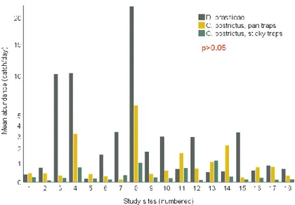
The relation between abundances of D. brassicae and C. obstrictus was examined with correlation tests. The test results did not show any significant correlation between abundances of D. brassicae and abundance of C. obstrictus in the pan traps (r=-0.063, n=18, p>0.05) or abundance of C. obstrictus in the sticky traps (r=0.034, n=18, p>0.05) at the study sites. Figure 15 display the mean trap catches of midges and weevils at the study sites.

(26)

21

Figure 15. Bar chart showing mean abundances of D. brassicae in sticky traps and mean abundances of C. obstrictus in sticky traps and pan traps at the study sites.

3.5 Differences in abundances of D. brassicae and C. obstrictus within- and

outside of the PFCZ

Differences in abundance of C. obstrictus in the pan traps and D. brassicae and C. obstrictus in the sticky traps obtained within the PFCZ and outside of the PFCZ was tested. The test results showed no statistically significant difference in abundance between the sticky traps for D. brassicae (Z=-0.849, n=18, p>0.05) or in the sticky traps for C. obstrictus (Z=-0.166, n=18, p>0.05) or in the pan traps for C. obstrictus (t17=1.208, n=18, p>0.05) at the study sites.

3.6 Relation of abundance of C. obstrictus between the trap types

The relationship between trap catches of C. obstrictus in different trap types was assessed in a correlation analysis. The test results demonstrate a positive correlation between the two trap types (r=0.496, n=18, p=0.036) (figure 16).

Figure 16. Scatter plot with regression line showing mean C. obstrictus trap catches from the two different trap types; yellow pan trap and yellow sticky trap at the study sites.

(27)

22

3.7 Difference in abundance of C. obstrictus between the season of 2017 and

2018

Difference in abundance of C. obstrictus between a study in the season of 2017 and

abundance in this study was examined. The metrics of mean catch/day for each season was compared. These comparisons only provide a general overview of the quantity of C.

obstrictus in this study compared to last year because the field methodology differ somewhat between the study in 2017 and 2018. In 2017, 19 fields were included and there were four sticky traps and two pan traps which were located at different borders of the fields, while in this study, there were 18 study sites with two sticky traps and two pan traps at each field and that were located at the same border of the fields (figure 7). Moreover, the traps were located in field during a longer period of time in this study and some of the study sites differs between the studies in 2017 and 2018.

Mean abundances (mean catch/day) of C. obstrictus in sticky traps in 2017 was 2.58, while it was 0.33 in the study in 2018. Mean abundance in pan traps was 12.50 in 2017 and 1.11 in 2018. There were often large variations in catches between the samples in the study in 2017 and in the study in 2018. The test results showed a statistically significant difference between the abundance of C. obstrictus in 2017 and 2018 for sticky traps (U=37, n=37, p<0.001) and for pan traps (U=23, n=37, p<0.001) (figure 17).

A B

Figure 17. Boxplots showing a general overview of mean abundance of C. obstrictus in sticky trap- and pan trap samples during the season of 2017 and 2018. The graphs display mean abundance of all the study fields in 2017 and 2018. 17(A): abundance in sticky trap samples. 17(B): abundance in pan trap samples. Note that the abundance have been log-transformed in order to also illustrate the differences between the samples.

(28)

23

3.8 Differences in within- field damages by D. brassicae in early- and late

pod set

Within- field differences in damages by D. brassicae at the field edge and 20m into the field within- and outside of the PFCZ in early- and late pod set was assessed. In order to display the extent of the spread and distribution of damages within the fields, all combinations tested are displayed in figures regardless if the tests show statistical significances or not.

Early pod set

Table 2 and figure 18 presents the results of the tests of differences in damage between the field edge and 20m into the field within- and outside of the PFCZ.

Table 2. Results of T-tests of differences in damage at the field edge and 20m into the field within- and outside of the PFCZ in early pod set.

Test early pod set

Within the PFCZ Outside of the PFCZ

Test value n p- value Test value n p- value

Field edge vs. 20m -0.032 (t) 18 >0.05 0.931 (t) 18 >0.05

A B

Figure 18. Bar charts of differences in damages between the field edge and 20m into the field in early pod set. 18(A): differences between the sample locations within the PFCZ. 18(B): differences between the sample locations outside of the PFCZ.

Differences in damages between the sample locations at the field edge within the PFCZ and the location at the field edge outside of the PFCZ, and the locations 20m into the field within the PFCZ and 20m into the field outside of the PFCZ, was also tested. Table 3 and figure 19 display these test results.

(29)

24

Table 3. Results of T-tests of differences in damage of the sample locations at the field edge within the PFCZ and at the field edge outside of the PFCZ and the sample locations 20m into the field within the PFCZ and 20m into the field outside of the PFCZ in early pod set.

Field edgewithin the PFCZ _{20m into the field}within the PFCZ

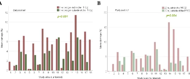
Field edgeoutside of the PFCZ _{4.573 (t)} _{18 <0.001} _- _- _- 20m into the fieldoutside of the PFCZ _- _- _- _{3.370 (t)} ₁₈ _0.004

A B

Figure 19. Bar charts showing within-field differences in mean damage by D. brassicae between the sample locations at the field edge and 20m into the field within- and outside of the PFCZ in early pod set. 19(A): differences between the sample locations at the field edgewithin- and outside of the PFCZ. 19(B): differences between the sample locations at the inner part of the fieldwithin- and outside of the PFCZ.

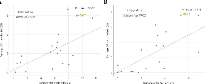
To assess the progression of damages between the field edge and 20m into the field within- and outside of the PFCZ in early pod set, correlation analyses were computed. Positive correlations were wound. Table 4 and figure 20 display these test results.

Table 4. Results of correlation analyses of damage at the field edge and 20m into the field within- and outside of the PFCZ in early pod set.

Within the PFCZ Outside of the PFCZ

(30)

25

A B

Figure 20. Scatter plots with regression lines of the relationship between mean percentage of damage at the field edge and 20m into the field within- and outside of the PFCZ in early pod set. 20(A): within the PFCZ. 20(B): outside of the PFCZ.

Late pod set

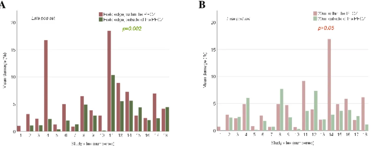
Since the study design in late pod set also included sample locations at the remaining borders of each test field apart from where the PFCZ was located, analysis of differences in damage between the edges and 20m into the field outside of the PFCZ includes two tests.

Unfortunately only 17 study fields could be included in the analyses that regarded analyses at the field edge outside of the PFCZ due to loss of sample notes of one sample point at the field edge outside of the PFCZ, during data compilation. Table 5 and figure 21 presents the results of the tests, where statistically significant difference was found between the field edge and 20m into the field outside of the PFCZ when samples at all the field borders were included in the analysis.

Table 5. Results of T-tests of differences in damage at the field edge and 20m into the field within- and outside of the PFCZ in late pod set.

Test late pod set Within the PFCZ Outside of the PFCZ* Outside of the PFCZ

Test value n p- value Test value n p- value Test value n p- value

Field edge vs. 20m

0.973 (t) 18 >0.05 0.659 17 >0.05 4.939 (t) 17 <0.001

* Includes only the sample locations at the field edge where the PFCZ was located.

(31)

26

C

Figure 21. Bar charts of differences in damages between the field edge and 20m into the field in late pod set. 21(A): differences between the sample locations within the PFCZ. 21(B): differences between the sample locations outside of the PFCZ when only the field border where the PFCZ was located are included. 21(C): differences between the sample locations outside of the PFCZ when all the field borders are included.

Differences in damages between the sample locations at the field edge within the PFCZ and the location at the field edge outside of the PFCZ, and the locations 20m into the field within the PFCZ and 20m into the field outside of the PFCZ, was also tested. Only the field border where the PFCZ was located are included in these analyses. Table 6 and figure 22 display these test results.

Table 6. Results of T-tests of differences in damage of the sample locations at the field edge within the PFCZ and at the field edge outside of the PFCZ and the sample locations 20m into the field within the PFCZ and 20m into the field outside of the PFCZ in late pod set.

Test late pod set Field edgewithin the PFCZ _{20m into the field}within the PFCZ

Field edgeoutside of the PFCZ* _{-3.053 (Z)} ₁₇ _0.002 _- _- _- 20m into the fieldoutside of the PFCZ* _- _- _- _{-1.459 (Z)} _{18 >0.05} * Includes only the sample locations at the field edge where the PFCZ was located.

A B

Figure 22. Bar charts showing within-field differences in mean damage by D. brassicae between the sample locations at the field edge and 20m into the field within- and outside of the PFCZ in late pod set. 22(A): differences between the sample locations at the field edgewithin- and outside of the PFCZ. 22(B): differences between the sample locations at the inner part of the fieldwithin- and outside of the PFCZ.