Trada Patterns in Eastern Europe : The Impact of Distance and the Customs Union Effect

Trade Patterns in Eastern Europe

The Impact of Distance and the Customs Union Effect

Master’s thesis within Economics

Author: Tina Alpfält

Tutors: Lars Pettersson, Ph.D.

Johan Larsson, Research Assistant Jönköping June 2010

Master’s Thesis in Economics

Title: Trade Patterns in Eastern Europe – The Impact of Distance and the Customs Union Effect.

Author: Tina Alpfält

Tutors: Lars Pettersson, Ph.D. & Johan Larsson, Research Assistant

Date: 2010-06-16

Subject terms: EU, Eastern Europe, trade, gravity model, customs union

Abstract

In 2004 the EU faced its most extensive enlargement ever when ten new countries joined. One can speculate about the reasons for these countries to join the EU and one suggestion that is often found is the access to a larger market and the trade possibilities that would entail; the customs union effect. Therefore this thesis sets out to investigate whether this is plausible; do countries trade more with the EU-countries than their non-EU neighbours? The investigation is conducted through the use of a gravity model. It investigates not only the traditional GDP and distance variables, but also the effects on trade flows caused by sharing borders, being part of the EU and sharing a language. The results show that not much could be seen in the trade flows in 2004; the year of accession. This could be attributed to the existence of preferential trade agreements, which the Eastern European countries had with the EU prior to their accession. It was also found that both the effect of sharing a language and the effect of increased distance are diminishing over the years. In addition a clear difference could be seen in the export from Eastern Europe to EU 15 and the rest of the world; it seems that some extra variables need to be added to explain the non-EU trade. Thus it can be concluded that the motivation for joining the EU should not have been the increased trade possibilities, but rather other factors such as regional development and the possibility to being part of a larger power at international negotiations.

Acknowledgements

Firstly, I would like to thank my tutors Lars Pettersson and Johan Larsson for their assistance throughout the writing process and my discussant Anneloes Muuse for her valuable comments.

Secondly, I am grateful to my good friends Cathrine Roos and Nicoleta Stepman who have spent time on reading and commenting my work.

Lastly, I am ever so grateful to my beloved Linus Wallin for all the support throughout this semester.

i

Contents

Acknowledgements ... ii

1

Introduction ... 1

2

The World Trade & the EU ... 4

2.1 Changing Patterns in the World Trade ... 4

2.2 The Creation and Development of the European Union ... 5

2.3 Trade Agreements of the EU ... 6

3

Trade Analysis based on Economic Integration ... 7

3.1 The Levels of Economic Integration ... 7

3.2 The Positive Effects of Integration ... 8

3.2.1 Tariffs ... 8

3.2.2 Comparative Advantages ... 9

3.2.3 Economies of Scale ... 9

3.3 Welfare Effects of Economic Integration ... 11

4

Trade Analysis Using the Gravity Approach ... 12

4.1 Tinbergen ... 12 4.2 Pöyhönen ... 13 4.3 Linnemann ... 13 4.4 Recent Developments ... 15 4.4.1 Theoretical Foundations ... 15 4.4.2 Econometric Specifications ... 17

5

Empirical Section ... 18

5.1 Presentation of Model and Variables... 18

5.2 Other Assumptions and Information ... 20

5.3 Econometric model ... 21

5.4 Descriptive Statistics ... 21

5.5 Regression Results ... 23

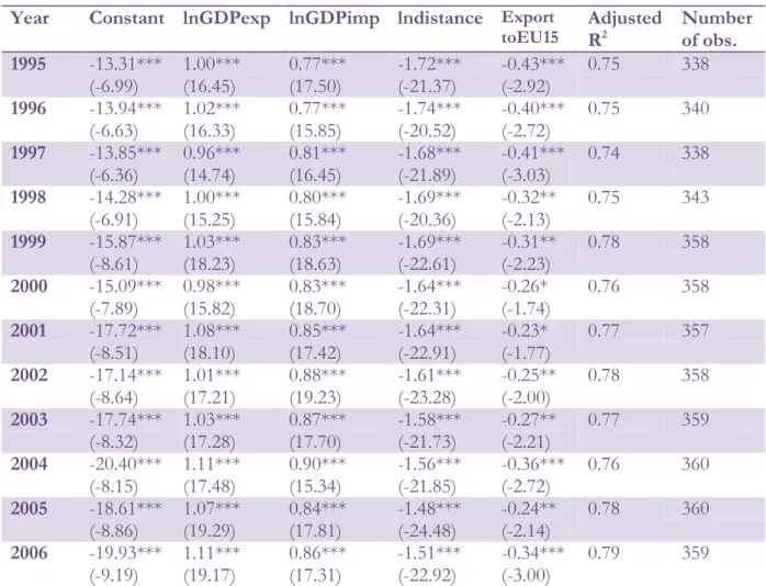
5.5.1 Results From Regression Set 1 ... 23

5.5.2 Results From Regression Set 2 ... 25

5.5.3 Results From Regression Set 3 ... 27

6

Analysis... 29

7

Conclusion ... 33

ii

Figures

Figure 1.1 Disposition. ... 3

Figure 3.1 Levels of economic integration ... 7

Figure 3.2 The tariff’s effect on the markets ... 8

Figure 3.3 Downward sloping average cost curve. ... 10

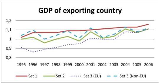
Figure 6.1 The observed trends in the coefficient of lnGDPexp. ... 30

Figure 6.2 The observed trends in the coefficient of lnGDPimp. ... 30

Figure 6.3 The observed trends in the coefficient of lndistance. ... 31

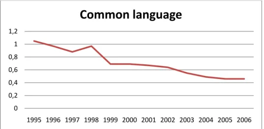
Figure 6.4 The observed trend in the coefficient of the dummy commonlanguage. ... 32

Tables

Table 5.2 Descriptive statistics 1995. ... 22

Table 5.3 Descriptive statistics 2006. ... 22

Table 5.4 Results from regression set 1. ... 24

Table 5.5 Results from regression set 2. ... 26

Table 5.6 Results from regression set 3. ... 28

Appendix

1

1

Introduction

May 1st 2004 was a special date in European history; after having had fifteen members for almost a decade the EU faced its biggest enlargement ever when ten new members joined1, mostly situated in the Eastern parts of Europe.

When the predecessor to the present EU was founded in 1951, it was originally a project of peace and security (Altomonte & Nava, 2005). According to Molle (2006) the way to promote peace and cooperation in Europe was to promote economic integration. Already in 1957 the next treaty created the European Economic Community (EEC), which aimed at removing trade barriers and creating a single market for the members.

By creating a customs union, like the EU has done, trade with the members of the union is promoted and increased. According to Badinger and Breuss (2004) the intra-EU trade has grown with approximately 6.7% per year, over the period 1960-2000. This could be attributed to, for example, greater possibilities of taking advantage of economies of scale and comparative advantages.

Since much of a country’s gain from joining a project such as the EU, and gaining access to the large European market, comes from its increased trade; it is of great importance to analyse whether this expected increase actually takes place. The existence of a customs union predicts increased trade with the other EU members without taking distance into account, whereas the gravity model predicts decreased trade with increasing distance. In order to analyse which effect is the strongest and most relevant for the European setting, especially for the new members in Eastern Europe, the purpose of this thesis is to answer the following research questions:

 Do countries that are situated in the outskirts of the EU trade more with their non-EU neighbours2 than with their fellow, non-neighbour, EU members? Thus, is the negative effect from the distance stronger than the positive effect of the customs union?

 And how are the effects of the variables changing over time?

The problem will thus be put in a setting of the EU, and the ten members who joined in 2004 will be of special interest since most of them are situated in the periphery of the EU. However, Cyprus and Malta, which are not part of the mainland Europe, are of small economic size and do not have any direct borders to its neighbours will be excluded from the study. Members of the Organisation for Economic Co-operation and Development (OECD), that are not already members of the EU, and the BRIC countries3 will also be included in the study4. The reason for including them is twofold; to get a larger sample and to get more variation of distances and trade volumes.

In addition, the study is subject to a few limitations. Firstly, only the years 1995 to 2006 will be used in order to minimise the risk of disturbances in the data due to other enlargements of

1

All members and their year of accession can be found in Appendix 1

2 _{The term neighbour always refers to first-order neighbours.}

3 _{BRIC = Brazil, Russia, India & China.}

2 the EU than the one in 20045. Secondly, not the same number of observations will be generated for each year due to data availability and changing trade patterns. Thirdly, only the categories of goods that are included in the Standard International Trade Classifications (SITC)6 revision 3, and hence collected by the database Comtrade will be included in the study.

1.1

Previous Research

A model often used for analysing trade flows is the gravity model. According to Krugman and Obstfeld (2009) “the value of trade between any two countries is proportional, other things equal, to the product of the two countries’ GDP’s, and diminishes with the distance between the two countries” (p.14). This suggests that countries that are situated close to each other should trade more than countries situated further apart.

An article regarding the importance of national borders for the size of trade patterns, which made use of the gravity model, was written by John McCallum in 1995. He studied the trade patterns over the USA-Canada border and found that even though the countries had a free trade agreement in place the trade between two domestic provinces was about 20 times larger than the trade across the national border. This is larger than a gravity model would predict in the case of no national border, according to McCallum (1995), who draw the conclusion that national borders matter even in the era of free trade agreements.

Many researchers have applied the gravity model to European studies. One example is an article by Papazoglou, Pentecost and Marques (2006) that tries to estimate the trade potential of Eastern Europe. The first step is to calculate the effects of the variables in the gravity model on the main trading partners of the EU. The second step is to use those coefficients and plug in the data for the countries in Eastern Europe. The calculated values give the trade potential of these countries. Then one can compare them with the actual trade flows in order to see if there is “more room” for trade with the countries in question or if the capacity is fully used. In addition to the ordinary gravity model variables, GDPi, GDPj and distanceij,

Papazoglou et al. (2006) included one dummy for common border and one for EU membership. The results indicated that trade with the EU 15 would increase, with an average of 12%, and trade with the rest of the world decrease. They also found that the export from EU15 to these new members would rise more than the import from them.

The same result was found by Buch and Piazolo (2001), who estimated the effects of the EU enlargement not only on traded goods but also foreign direct investments (FDI), portfolio investments and other banking assets. Their regression results indicate that the accession to the EU should pose a significant and positive effect on the capital flows and trade between these ten new members and the EU 15.

Bussière, Fidrmuc and Schnatz (2008) used the potential trade approach as well. They used, like Papazoglou et al. (2006) a dummy to indicate if two countries share a border and if they are part of a free trade area (FTA). In addition, they added two more dummies; one to indicate

5 _{Sweden, Finland & Austria joined on January 1, 1995 and Romania & Bulgaria on January 1, 2007.}

3 whether the countries use a common language and one to indicate if the countries have been part of the same territory previously. Their results are stable for the ordinary gravity model variables but the result for the EU dummy varies; sometimes it is found to be insignificant. The conclusions drawn by Bussière et al. (2008) are that in the beginning of the economic integration with these countries, in the early 1990’s, the trade volumes were lower than expected. Nevertheless, this has changed over the years where a convergence towards more “normal” levels of trade has been observed. This suggests that the additional scope for integration and increased trade with these new EU members may be limited. The same conclusions are drawn by Gros and Gonciartz (1996) and Nilsson (2000).

An article by Breuss and Egger (1999) evaluates the accuracy of the method of using trade potentials. They reach the conclusion that this method is not appropriate since the prediction intervals they calculate show variations up to 350%. Egger (2002) suggests that the existence of positive trade potentials is a sign of model misspecification. However, he thinks the model is useful for simulations and suggests focus being put on changes in the explanatory variables and their effect on the trade values. Therefore this thesis will not make use of trade potentials, but rather use cross-sectional regression to investigate the development over time in the variables studied. No previous studies have been found that conduct this type of study.

1.2

Disposition

The next chapter contains the background, Chapter 2. It brings up the issue of world trade and what patterns can be seen together with a description of various aspects of the EU. The theory section includes two chapters which is necessary in order to understand the reasoning behind the two different theories mentioned previously. Chapter 3 discusses the effects of economic integration and Chapter 4 describes the gravity model and its development over time.

Chapter 5 describes the model and method used to derive the results, which is continued in Chapter 6 with an analysis of the results, with respect to what has been learned earlier in the thesis. Finally, the most important findings are presented in the conclusion in Chapter 7, together with some suggestions for further research. A visual overview of the thesis can be seen below in Figure 1.1.

4

2

The World Trade & the EU

2.1

Changing Patterns in the World Trade

In general trade has increased over the last decades. According to the Worldwatch Institute, the trade in goods and services expanded from about 5 trillion US dollars in 1990 to almost 10 trillion US dollars in the middle of the 2000’s. These values have been calculated in 2003 constant US dollars in order to remove the effect of the inflation (Worldwatch Institute, 2005). Besides from this general increase in trade volumes other trends have been observable. The first trend is the increased importance of services both in domestic production and the world trade. According to Krugman & Obstfeld (2009) almost 20% of the world trade in 2005 consisted of services and that share is expected to rise in the future. The World Trade Organisation (WTO) states that the service sector is the fastest growing sector in the global economy (WTO, 2010a). It is also the sector that employs the largest share of workers around the world; around two thirds of the labour force. The importance of this sector, and the free trade of its products, was recognised in the 1990’s and as a result the General Agreement on Trade in Services (GATS) was established in 1995 (WTO, 2010a). That the global economy, or at least part of it, has moved towards this kind of trade is not very surprising when looking at the model of Rostow’s five stages of economic growth (Rostow, 1960). The fifth, and last, stage is called the age of high mass-consumption and the important change, compared to the previous stage, is that the manufacturing industries that used to be prosperous are being replaced by service industries.

A second trend seen is that more and more of the world trade is becoming intra-firm trade. A report by UNCTAD states that there were about 45 000 transnational corporations (TNC) operating in the world in 1996 (UNCTAD, 1997). Together these parent firms have about 280 000 affiliates all around the world. As mentioned by UNCTAD, this method of opening up an affiliate and produce internationally is becoming a more common alternative to exporting ready goods (UNCTAD, 1997). In another report, in the same series, one can see that the figures have been rising sharply; in 2004 there were 70 000 parent firms operating about 690 000 affiliates globally (UNCTAD, 2005). According to Dicken (2007) there are three characteristics of a TNC that explain why. Firstly, a TNC has an ability to control and administrate production and other activities all around the world. Secondly, the TNC has the ability to make use of differences between countries, both in production factors and state policies. Thirdly, the TNC has a great flexibility when it comes to locations. It can move resources and tasks between affiliates or create new ones. When the TNC operates its goal is always to maximise profit, therefore operations are moved to where they are cheapest, or most advantageous to perform (Dicken, 2007). These international movements can have large impacts on the local communities that are involved.

The third trend that has been observed during the 1990’s and onward is the large increase in number of preferential trade agreements established; both bilateral and multilateral (Dicken, 2007). As an example he says that more than half of the preferential trade agreements reported to WTO up to 2004 were established after 1995.

The fourth trend discussed is the rise of Eastern Asia. Traditionally North America and Europe have played large roles in international trade, however, during the last few decades Asia has become more and more important (Dicken, 2007). As he puts it; “Without any doubt, the most significant global shift in the geography of the world economy during the past 40

5 years has been the resurgence of Asia – especially East Asia” (p. 43). This, he states, is due to four reasons; the large economic growth in Japan after the Second World War, the rapid growth of a few small countries called the Asian tigers, the large growth potential of India and the market orientation of China. Especially China has grown at magnificent rates and is the fourth largest manufacturing producer and second largest agricultural producer in the world by the early 21st century (Dicken, 2007).

2.2

The Creation and Development of the European Union

In the post-war period the economic integration, not only in Europe but also globally deepened. The United Nations was founded in 1945 (United Nations, 2010) and in 1947 the first trade round, establishing the General Agreement on Tariffs and Trade (GATT), was held in Geneva (WTO, 2010b).

Looking back at the first half of the 20th century it became clear for some European countries that the only way forward was to integrate and help each other (Molle, 2006). In 1950 the French foreign minister Robert Schuman held a famous speech, the Schuman Declaration, where he suggested that France, Germany and other countries, that would find it in their interest, should pool their coal and steel resources. The suggestion was appreciated and accepted by not only Germany and France, but also Italy, Belgium, Luxembourg and the Netherlands. Hence a treaty was signed in 1951 in Paris and in 1953 the European Coal and Steel Community (ECSC) came into force (Altomonte & Nava, 2005). Only a few years later, in 1957, these six countries decided to deepen their cooperation. Therefore two new communities were created; the European Atomic Energy Community (EURATOM) and the European Economic Community (EEC). As explained by Altomonte and Nava (2005), these three communities had had three different organisations, which was very inefficient. Thus it was decided in 1967 that these should merge into one organisation only, where there would be a commission working for the interest of the community as a whole.

The discussion of deepening the economic integration continued and in 1968 a common external tariff was decided upon, thus a customs union had been created in Europe (Altomonte & Nava, 2005). With the tariffs abolished, other non-tariff barriers to trade became apparent; some examples are national procurement and differences in technical standards. National procurement is when a government prefers to purchase domestic goods over foreign cheaper goods (Molle, 2006). Technical standards are not discussed as much as traditional barriers to trade but have the possibility to divide markets and impede trade between them. Different voltage requirements for electrical products and differences in allowed levels of various substances in food are some examples of this (Chen & Mattoo, 2008). The commission has worked a lot on these issues in order to complete the single European market (Molle, 2006). For example many regulated products have received a general-EU requirement instead of several national ones, and in other cases mutual recognition agreements have been formed (Chen & Mattoo, 2008).

The succeeding step in the integration process did not arrive until 1986, when it was decided that the member countries should form a single market. The remaining obstacles were removed thus creating the four freedoms; free movement of capital, labour, services and goods (European Union, 2010a). Related to a well-functioning single market is the existence of free competition. As described by El-Agraa (2007), the EU therefore prohibits certain uncompetitive behaviour. Cartels trying to form agreements about market shares and price levels are prohibited by EC law. It is also illegal to abuse one’s power if situated in a

6 dominant position; by exploiting consumers and exclude others from competing on the market. Firms that intend to merge have to notify EU beforehand so that an evaluation of whether it will harm the competition on the market can be made. If it is found that the competition would be harmed the Commission has power to veto the merger (El-Agraa, 2007).

Several new treaties have been signed after The Single Act in 1986 and they have all sought to extend the cooperation into new policy areas and deepen the ones already existing, such as; environmental protection, and harmonization of economic and social policies (Molle, 2006). Another example is the creation of transport policies, which were seen as important for future development, due to the importance of infrastructure on trade. Shipping and air transport are two sectors that had been protected for a long time but were deregulated by the EU and thus forced to adjust to free competition (El-Agraa, 2007). The EU has also developed an energy policy, an environmental policy and is more and more concerned with social policies such as; employment, industrial health and social protection (El-Agraa, 2007). Another area that has received a lot of attention is regional development, which is made possible through the fiscal federalism that redistributes money from the wealthy regions to the poorer regions. After the two last accessions of members in 2004 and 2007 the regional disparities have grown substantially, requiring developments of the regional policies (El-Agraa, 2007).

2.3

Trade Agreements of the EU

“The EU is firmly committed to the promotion of open and fair trade with all its trading partners.” This can be read on the EU’s official webpage (European Union, 2010b).

As stated, the EU tries to promote free trade, in excess of the multilateral agreements that are negotiated in the WTO’s rounds. The agreements are reported to the WTO and noted under two different articles; XXIV in GATT if the agreement concerns trade in goods and article V in GATS if it concerns trade in services. What is approved to trade under each agreement varies; however, generally the EU restricts free trade with agricultural products.

There are three groups of trading agreements the EU has negotiated over the years. Firstly, there are bilateral agreements with other trading blocs such as Mercosur, and the Gulf region (European Union, 2010c). Secondly, there are bilateral agreements with other countries such as Turkey, Norway and the USA (European Union, 2010b). Thirdly, there is a special group of short-term agreements, Europe agreements, which are supposed to prepare a country for accession to the EU (Breuss & Egger, 1999; Council of the European Union, 2010).

The implications of these preferential trade agreements are that, not only can the countries within the EU trade with each other without facing any tariffs or quotas, but they can also trade with many non-EU countries without facing these tariffs. This could have important implications for this study and its result. For a complete list of the trading agreements the EU has negotiated see Appendix 4.

7

3

Trade Analysis based on Economic Integration

3.1

The Levels of Economic Integration

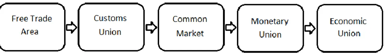
There are various levels of economic integration, as can be seen in Figure 3.1. These are described by McDowell, Thom, Frank and Bernanke (2006) and they are very similar to those steps described by Balassa (1962).

Figure 3.1 Levels of economic integration (Author’s own construction, based on McDowell et al., 2006)

The first step of economic integration is to create a FTA. The implications of this are that the member countries can import goods from and export goods to each other without paying tariffs or being subject to quotas. However, the member countries are free to set the tariffs and quotas facing the countries that are not members of the FTA in a way they find appropriate (Balassa, 1962).

As McDowell et al. (2006) explain pressure will arise for moving towards a customs union if a FTA is already set in place. Since the countries in the free trade are allowed to have different tariffs against the non-members, the country with lowest tariff will most likely become a transit country. Non-member countries export their goods via that country and when inside the FTA the goods can move freely without tariffs between the member countries. This creates problems in defining the origin of goods and additionally, the countries in the FTA with higher tariffs may lose revenues since the imported goods are being redirected. The remedy to this situation is for the countries to agree upon a single tariff facing non-members; hence the FTA develops into a customs union.

When the customs union is formed pressure to move towards a higher level of integration will arise. Weststrate (1948) gives examples related to labour markets and wage policies which show that a country cannot pursue independent goals without affecting the other members. In addition, when the goods and services are allowed to flow freely countries may put restrictions on other factors, in order to protect domestic industries, according to McDowell et al. (2006). This problem can only be solved if the two remaining factors, labour and capital, are allowed to move freely within the union as well. The customs union then develops into a common market.

There are always risks related to exchange rate movements when trading with non-domestic actors. The uncertainty created by the constant changes in the exchange rates may impede trade. In addition a fixed exchange rate can be manipulated by the government to benefit the domestic firms, through devaluations and other monetary operations (McDowell et al., 2006). The solution is to adopt a common currency and to coordinate the monetary policies, which also means that the common area transforms and becomes a monetary union.

8 When having a common currency there is of great importance that the countries coordinate other policy instruments, such as taxes, regulations of cartels and foreign policy according to Weststrate (1948). As he explains; economic policy is closely related to general policy. Thus the final level is reached; an economic union has been created. Both Weststrate (1948) and Balassa (1962) suggest that at this final level a supranational body could be of use.

3.2

The Positive Effects of Integration

Creating a lager economic unit such as a customs union has positive effects that do not stem from the actual creation but from other economic phenomenon. As seen in Chapter 3.1., the first step of economic integration concerns the removal of tariffs; hence the positive effect on trade is a result of the abolished tariffs and not the existence of a union per se.

Other effects that are related to economic integration are, according to Balassa (1962), results of the access to a larger market. This allows for higher specialisation through utilisation of comparative advantages and economies of scale.

3.2.1 Tariffs

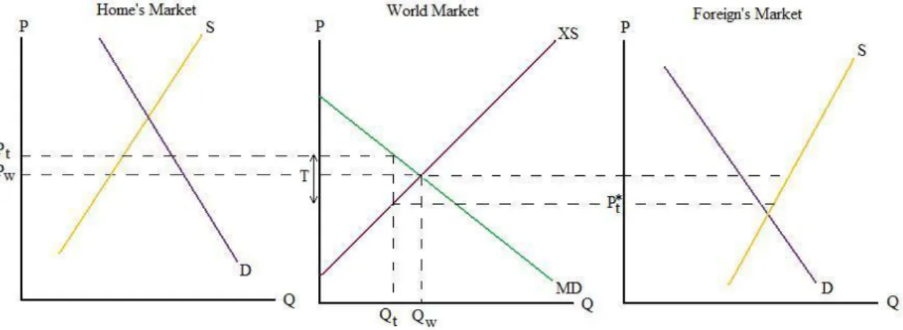
A tariff can be regarded as a tax on imported goods and can either be specific, a fixed sum per unit of good, or an ad valorem tax, a percentage of the value of the goods (Krugman & Obstfeld, 2009). Imposing a tariff on a good is usually done to protect a domestic industry from cheaper imports; however, this is an obstacle for free trade and therefore imposes costs on the country. As can be seen in Figure 3.2., imposing a tariff will raise the domestic price of the good. Pw is representing the world price that would prevail in both countries under free

trade, Pt is representing the price the domestic consumers will have to pay due to the tariff and

P*t the price the foreign country receives when selling the good.

Figure 3.2 The tariff’s effect on the markets (Source: Author’s own construction based on Krugman & Obstfeld, 2009).

9 The higher price on the domestic market results in higher domestic supply and lower domestic demand; hence the amount of the good that is necessary to import to satisfy the demand decreases. The opposite happens in the exporting country; the lower price raises the domestic demand and lowers the domestic supply; resulting in a smaller quantity that is available for export.

The result of this scheme is that the tariff places a wedge between the price in the foreign country and the domestic country. As mentioned by Krugman & Obstfeld (2009) the effect of the wedge differs due to the countries’ size on the world market. If the importing country is relatively small it will not be able to have the reducing price effect on its trading partner; hence, the price increase in the domestic country will be larger to incorporate the whole size of the tariff and the foreign consumers will not see any domestic changes.

3.2.2 Comparative Advantages

In the early 19th century David Ricardo (1817) developed the theory of absolute and comparative advantages. A country that can produce something more efficiently than another has an absolute advantage. The comparative advantage is not as intuitive and is therefore demonstrated with an example involving England and Portugal:

Ricardo (1817) assumes that in England 100 men would be needed for a year to be able to produce a certain amount of cloth. To instead produce wine would require 120 men for a year. In Portugal the labour requirements for production of the same quantities of cloth and wine are 90 and 80 respectively. Hence, Portugal has absolute advantages for the production of both goods. Nevertheless, trade can still be beneficial since Portugal can, by focusing its production on wine, use the labour of 80 men and trade their wine output for the amount of cloth it would take 90 men’s labour to produce. England can devote the labour of a 100 men and trade their cloth output for a quantity of wine that requires 120 men’s labour. The conclusion Ricardo (1817) draws is that this trade is mutually beneficial although at a first glance Portugal would appear the best producer of both goods.

The optimal rule of specialisation is thus to specialise in the good for which the country in question is the least bad at producing; has a comparative advantage in. In an area with no tariffs or other obstacles to trade these comparative advantages can be fully utilised which would lead to a higher efficiency in production and a larger union output. According to Balassa (1962), this more efficient production would lead to a higher welfare in the union.

3.2.3 Economies of Scale

Economies of scale, or increasing returns to scale, is a phenomenon that refers to a situation where increasing the output results in a lower average cost per unit produced (Brakman, Garretsen & van Marrewijk, 2001). This is depicted in Figure 3.3.

10 Figure 3.3 Downward sloping average cost curve. (Author’s own construction)

The demand curve for an individual country is represented by DC and the demand curve for an

entire union is represented by DU. The demand for the union is located to the right of the

national demand since that market is larger. This allows the firm to produce at a lower cost due to the shape of the average cost curve. There may be several reasons for the average cost curve to have this downward sloping shape and they are usually divided into two categories; internal economies of scale and external economies of scale.

The internal economies of scale are, as the name suggests, internal to the individual firm and is a result of increased output. The higher the level of production, the lower is the average cost. This could be due to several reasons, such as; the construction of for example pipelines has a relationship between cost increase and capacity that is larger than unity, if the surface area required for the construction doubles the capacity of the pipeline will more than double (Varian, 2006). Other examples are the possibility to handle and ship the goods at a larger scale, which usually increases the costs less than proportionally, and the fact that a large scale production may be necessary for warranting the use of special equipment and specialised labour. In addition, some costs are not proportional to the production level; this is usually the case for design and research (Balassa, 1962).

The external economies of scale may be divided into two categories; pure and pecuniary. The pure external economies of scale are results of technological improvements that increase the output at industry-level. One example highlighted by Brakman et al. (2001) is information spillovers. New knowledge in the industry will spill over and reach the individual firms. The pecuniary external economies of scale are dependent on markets and prices. Examples are the existence of a market with specialised labour and the existence of specialised subcontractors. If a subcontractor makes a new innovation that results in its goods being cheaper, the firm purchasing these intermediate goods will gain as well.

Balassa (1962) claims that, especially the external economies of scale are important for integration projects, such as customs unions, since they enable firms to specialise and produce larger quantities. As he puts it; “the wider the market, the larger will be the economies of specialisation” (p.157).

11

3.3

Welfare Effects of Economic Integration

Whether the net effect of creating a large economic unit, such as the EU, is positive or negative depends on whether the utilisation of economies of scale and comparative advantages, in the absence of tariffs, give rise to trade creation or trade diversion. Trade creation refers to the new trade that is initiated when countries become members of the same FTA or customs union. Trade diversion is referring to a case where a good that was previously imported from a certain country is, after the creation of the union, replaced with a good from another member country even though the initial good was cheaper and more efficiently produced (Viner, 1950).

Which one of these two effects that is the largest has to be calculated on a case-by-case basis. However, Balassa (1962) mentions that successive increases of the size of a customs union should at least reduce the risk of trade diversion. In addition, he summarises a few characteristics that increase the likelihood of a customs union having a positive effect on the world’s welfare. Some of the mentioned ones are; the competitive structure in the member countries, high levels of tariffs prior to the establishment of the customs union, large differences in production costs between the member countries, a large size of the union and short distances between the member countries.

Without making a thorough examination of the EU it is quite clear that at least some of these characteristics are present. For example the EU presently consists of 27 member countries (European Union, 2010d) out of the total 49 countries in Europe7 (Encyclopædia Britannica, 2010). In terms of population size the EU incorporates 495 million of the continents total 732 million inhabitants (European Union, 2010d; Nationalecyklopedin, 2010). The EU also has developed polices to enhance free competition which has resulted in bans of cartels and other uncompetitive behaviour (Molle, 2006).

7

This figure includes countries that are only partly situated in Europe, such as Turkey and Russia, and the small states of Monaco, Andorra, San Marino, the Vatican City State and Liechtenstein.

12

4

Trade Analysis Using the Gravity Approach

4.1

Tinbergen

In the early 1960’s the Dutch professor Jan Tinbergen (1962) made a study regarding the world economy and how to optimally shape it by economic policies. He stated that optimum trade is equal to free trade if four conditions are provided. Firstly the income should be redistributed among and within countries, to some extent. Secondly, only temporary subsidies are to be given to infant industries. Thirdly, the subsidies should be given to vital industries only. Lastly, workers should be retrained and capital transferred from old to new industries. To find out whether a country is in a situation of optimal trade one could estimate the total value of trade between the country in question and a trading partner and then compare that value with the actual total trade value.

Tinbergen (1962) then assumes that the estimated figure will depend on a few general characteristics of the two countries; namely the size of the countries and the distance between them. The GDP of the exporting country is a sign of their capacity to produce and provide products. For the importing country the GDP has two interpretations; the first is a sign of the demand for imported goods and the second a sign of the degree of diversification of the country’s production. The distance is representing the costs related to transporting goods from one country to another. The result is a model, which is seen in Equation 4.1, that is positively related to the GDP of the two countries, albeit less than proportionally for the GDP of the importing country, and negatively related to the distance between them.

(4.1)

E represents the export from country i to country j, Y represents the GDP of each country respectively, D represents the distance between them and a0 is a constant. Since this model is

non-linear in the parameters it is easier to rewrite it for estimation purposes and the logarithmic version of the model can be seen in Equation 4.2.

(4.2)

This logarithmic model was used by Tinbergen (1962) for an empirical study of 18 countries, using data from 1958. The results showed that all variables were significant and all of them had the expected sign. A second attempt was made where some dummy variables were included; one for neighbouring countries, one indicating British Commonwealth preference and lastly one indicating Benelux preference. The only one that showed to be significant of these additional variables was the dummy for Commonwealth preference.

Another interesting finding by Tibergen (1962) was that the estimated coefficient a1 was

about 0.1 units larger than the estimated a2, which implies that the exporter’s GDP explains

more of the variation in trade than the importer’s GDP does. This confirmed his suspicions that the two interpretations of this variable would cause it to have a lower impact than the GDP of the exporter.

13

4.2

Pöyhönen

At the same time as Tinbergen (1962) developed his model the Finnish professor Pentti Pöyhönen (1963) independently worked at another version that was published a year later. He used a different approach when developing the model; he used matrices of exchanges of goods, national income and transport distances. However, in order to be able to use the model for empirical regressions he had to put it in a more general form such as the one seen in Equation 4.3.

(4.3)

The a’ij represents the estimate of export value between country i and j. The first c is a

constant, the second, ci is a parameter of the exporting country, and the third, cj is a parameter

of the importing country. In the upper part of the fraction, the e: s are representing the national income of the country i and j and the α and β associated with them are representing the income elasticities of imports and exports. In the lower part of the fraction the γ is a coefficient that represents the cost of transportation per nautical mile, the rij is the distance

between country i and j and lastly the δ is an isolation parameter.

Ten European countries were used in the empirical study, based on the quest for using water transportation as mode of transport, and performed on data from 1958. Some landlocked countries thus had to be excluded. The results showed that both income elasticities were positive, the γ was small, but positive; indicating that for every additional nautical mile of transport the negative effect grows larger.

As discussed by Pöyhönen (1963) in the end of the article, the model bears much resemblance with the gravity attracting bodies of mass to each other. Many other areas of economics have been shown by regional studies to have analogies in natural sciences and his empirical study convinced him that this analogy exists for the distribution of a country’s exports as well.

4.3

Linnemann

A few years after Tinbergen (1962) and Pöyhönen (1963) came up with the gravity model another Dutch professor named Hans Linnemann (1966) developed it further to include more variables. He also devoted more space to discussing the effects of the variables and why they should have a certain impact on the trade volumes.

Linnemann started off by dividing the variables explaining trade into three categories. The first category included variables that affect the potential supply exporting country, which he called country A in the discussion. The second included variables explaining the potential demand of country B. The third category was the trade resistance between country A and B. The first two categories are of more domestic nature and they do not vary with products or trading partners, in addition Linnemann (1966) assumed that the demand of country B depended on the same variables as the supply of country A. However, the last category is a bit different since transport costs usually vary with type of good, country and distance.

14 Then Linnemann (1966) asked himself why countries trade in the first place. The answer he found was that the domestic production was different from the domestic demand. A solution to this could be to change the production domestically so that it matches the demand. Nevertheless, this was ruled out due to comparative advantages that countries develop in a number of goods only. The result is that a country will produce a certain number of goods both for its domestic market and for foreign markets. Thus, a country’s foreign supply depends on its national product divided with a ratio of the domestic market and the foreign market as can be seen in Equation 4.4.

(4.4)

Another assumption made was that the trade resistance was equal for all countries. Under this condition the domestic-market/foreign market production ratio will vary with the population sizes of country A and country B. To convince his readers Linnemann (1966) uses two examples. The first comprises two countries with equal population sizes but different levels of income. The country with the higher income will have a higher demand, both for domestic and for foreign goods, hence the production ratio can be said to be about the same for both countries. In example two, the countries have the same income levels but their population sizes differ. The country with the larger population will have the possibility to pass the minimum market size required for efficient production for more goods than the country with the smaller population. Therefore the country with the larger population will have a higher domestic-market/foreign market production ratio.

At one point Linnemann (1966) suggests GDP per capita as a variable as well, but concludes that it may be difficult to incorporate this variable when both GDP and population are previously included in the model due to possible problems with multicollinearity. Another variable that is contemplated but disregarded is land area. The reasons for not including it are; the limited importance of natural resources since they are themselves traded as goods, the fact that people tend to agglomerate close to natural resources and that population size is found in the model already and lastly that size is not necessarily correlated with natural resources. The trade resistance can be attributed to two groups of obstacles. The first is comprised of natural obstacles and the second of artificial obstacles. With natural obstacles Linnemann (1966) is referring to transportation costs, the longer the distance the more costly to transport goods, additionally the longer the distance the more time it takes to transport goods. A third issue is the psychic distance, one generally knows more about the markets that are situated nearby and one may have a language in common. All three thus depend on the distance and therefore the distance is incorporated in the model to represent natural obstacles. The artificial obstacles consist of import duties and restrictions of quantities allowed to import. If one assumes that the trade-reducing effect caused by the tariffs and quotas is normally distributed, all trading partners are assumed to face the same average effect. Some countries might be facing deviations from that pattern but that is a consequence of randomness and is not changing the pattern. If all countries are assumed to face the same trade-reducing effect there is no need for a separate variable representing artificial obstacles, Linnemann (1966) reasoned.

There are some exceptions to this generality, which are not caused by randomness, and they are; communist countries that do not follow the same trade pattern as non-communist countries, countries facing embargos and lastly countries that are part of FTA: s or customs

15 unions. In an empirical study, countries falling into the first two groups should be excluded, however, countries being part of trade blocs can be included if they are being corrected for with a dummy variable (Linnemann, 1966).

The model suggested by Linnemann (1966), looks like Equation 4.5 in its simplest form. Thereafter a more elaborate version that includes a dummy for preferential trade agreements can be seen in Equation 4.6.

(4.5)

In this equation the X represents the export from country i to country j, E represents the potential supply, M the potential demand and R the resistance.

(4.6)

In the more elaborate equation the Y: s represent GDP, the P preferential trading agreement, the N: s population sizes and the D geographical distance. In order to make it linear before using it for empirical purposes the logarithmic version of the model is used and can be seen in Equation 4.7, when disregarding the negative signs on the coefficients that were found in the lower part of the previous model, Equation 4.6.

(4.7) Linnemann (1966) used data from 1959 for 80 countries and found that all variables were significantly different from zero. The GDP variables were both positive as expected, population size had a trade-reducing effect as expected and the same was the case for distance. The dummy for preferential trade agreement also showed to be positive.

4.4

Recent Developments

Since the 1960’s much research has been spent on developing the gravity model in various directions. Many researchers claim that there are no theoretical foundations behind the gravity model, such as Leamer and Stern (1970). Therefore some economists have tried to find a way to link the gravity model to economic theories, due to the lack of such links (Anderson, 1979; Bergstrand, 1985). Another group of researchers have worked towards improving the econometric stability of the model, which they have done by modifying the standard versions of the model to be less biased.

4.4.1 Theoretical Foundations

To the first group of economists, the one that studies the theoretical foundations of the model, one can count James E. Anderson who in an article from 1979 tries to find a theoretical explanation to the gravity model by assuming; identical homothetic preferences in all regions examined and that the goods can be differentiated by their place of origin. The share of income spent on tradeables is an unidentified function of the country’s population and

16 income. The total expenditure on tradeables in all regions will be a function of the cost of transporting them. This sounds reasonably similar to the gravity model proposed previously. Anderson (1979) then moves on to showing how the simple form of the gravity model stems from rearranging a Cobb-Douglas system of expenditures. The assumption is that each country has specialised in one good and that their identical preferences cause the share of income spent on a certain good to be identical for all countries examined. This, as presented in Equation 4.8, gives the gravity-like equation seen in Equation 4.5, where the income elasticities are assumed to equal unity.

(4.8)

By developing it a bit further to allow for different fractions of traded and non traded goods between the countries and non-unity of the income elasticities Anderson (1979) reaches another equation that resembles a gravity model, Equation 4.9. The ϕ represents the share of income spent on tradable goods and the Mij the demand of a tradable good from country i to

country j.

(4.9)

In 2003 there was another article by Anderson and van Wincoop that continued along this path of connecting the gravity model to theory. A difference between this new development and the work done in Anderson (1979) is that prices have been included and a variable representing the cost of trading, see Equation 4.10.

(4.10)

The σ represents the elasticity of substitution between all goods, the t the cost of trading, the P: s the price indices of country i and j and the y: s represent income of country i, country j and the world.

Bergstrand (1985) is another economist that tries to connect the gravity model to economic theory. He assumes that there is one factor of production in each country in the model, which is derived from utility-maximising behaviour and profit-maximising behaviour. The trade flow will thus be a function of the available resources of the countries studied in a given year and the transport costs plus trade-barrier costs between each country pair. By using this, and making some simplifying assumptions a model that is similar to the basic gravity model is found, and is shown in Equation 4.11.

(4.11)

The PXij represents the US dollar value of the export flow from country i to country j.

However, the model he used for his empirical study only made use of the first two assumptions; therefore the model became very large and included many variables. Some examples are GDP deflators and an exchange rate variable. Nevertheless he concludes that, if one is missing data on prices and exchange rates, a gravity model looking like Equation 4.2 can be used instead together with additional dummies needed for the situation at hand.

17 4.4.2 Econometric Specifications

The second group of economists have claimed that the frequently used basic gravity equations, such as those in Equation 4.2 and Equation 4.7, are misspecified. One of them is László Mátyás (1997) who uses triple indices instead of double, as most other economists described previously in the thesis, he also uses three categories of intercepts. The model thus looks like the following, Equation 4.12.

(4.12)

In this equation α represents the effects specific to the exporting country, γ is the equivalent for the importing country and the λ is the year specific effects. The dependent variable represents the natural logarithm of the export from country i to country j in year t, similarly the DIST represents the natural logarithm of the distance between country i and j, and the u is representing an error term.

This model is a general model that can be used in various ways depending on which restrictions one put on it. If having a cross-sectional data set the λt will be equal to zero. The

αi and the γj will vary with the countries studied, hence allowing for them to differ, which the

basic model does not allow and therefore result in biased estimators.

The same argument has been put forward by Cheng and Wall (2005); however, they claim that the model proposed in Equation 4.12 will provide biased results as well. As they explain, an exporting country does not have the same relation to all importing countries. Therefore, what is really needed is a dummy for each country pair, assuming that αij≠αji. If using this

approach the least square dummy variable model (LSDV) can be used to estimate the coefficients from the model shown in Equation 4.13.

(4.13)

The β´Zijt represents the usual gravity equation variables; the GDP, the population and the

distance. Cheng and Wall (2005) perform an empirical study where they compare the models proposed by, among others, Linnemann (1966) and Mátyás (1997). Their results show that the model proposed in Equation 4.13 generates the results with the best fit.

18

5

Empirical Section

5.1

Presentation of Model and Variables

From the beginning of this study a gravity equation was intended to be used as model, however, as shown in Chapter 4 there are numerous versions of the gravity equation. The first choice fell on the Equation 4.13, as developed by Cheng and Wall (2005). Nevertheless, with the limited range of years in this study the degrees of freedom would be too low if using that model. The second choice thus fell on the model developed by Linnemann (1966), due to his appealing explanations of how both GDP and population are important factors for describing trade. A correlation matrix was computed to investigate whether there were any variables one needed to be careful with. The results showed that GDP and population among the countries in the sample were correlated with approximately 75-77%, depending on year. The population variables were therefore disregarded and the models used instead are modified versions of Tinbergen’s (1962) model, Equation 4.2.

Due to the problem investigated in this study one set of regressions is not sufficient to be able to draw conclusions about the variables and their effects. Therefore three sets were performed and are presented below.

The first set uses Equation 5.1., which is the full model including all variables intended to study. The set also make use of all 46 countries in the sample.

(5.1)

The second set has a smaller sample; only the eight countries that entered the EU in 2004 in the sample are used. The focus is on the core variables of the gravity model, as formulated by Tinbergen (1962), with one dummy indicating trade with the EU 15; which is equivalent to Equation 5.2. This is done in order to investigate whether the importance of trade with the “old” EU members increases as these eight countries enter the EU.

(5.2.)

The third set uses this smaller sample as well, however, this time the sample is split and two regressions are performed; one that contains trade with the EU-15 and one that contains trade with all other countries making the model look like Equation 5.3. In this regression set pair wise comparisons can be made to detect any differences in the variables that depend on trading partner.

(5.3)

The variables used in the models are presented below, together with their sources and expected signs. A summary of the hypotheses can be found in Table 5.1, after the variables have been presented.

Export Value (lnexpvalue)

This is the dependent variable of the model and the data was collected from Comtrade, a database containing international trade statistics maintained by the UN. In Comtrade the

19 values extracted are the total exports from one country to the other 45 in the study and the unit used was the monetary value in current US dollars; since weight is neither practical nor available as unit of measure when aggregating different goods.

GDP of the exporting country (lnGDPexp)

This explanatory variable was collected from the UNdata database and is stated in current US dollars. As explained by both Linnemann (1966) and Tinbergen (1962) this variable should have a positive impact on the export value, since the higher production (GDP) a country has the larger volumes could be exported.

GDP of the importing country (lnGDPimp) A This explanatory variable was collected and measured in the same manner as the previous variable; the GDP of the exporting country. The variable is expected to have a positive impact on the export value as well, since higher GDP means higher income and thus higher demand of products, not only of domestic goods but also of foreign goods (Linnemann, 1966).

Distance (lndistance)

This explanatory variable was collected from the World Atlas online application, where the distance, as the crow flies, in kilometres between two cities can be found. The cities chosen for this study were in most cases the capitals of the countries in the sample. However, in some cases the largest city, measured by population, in each country was chosen. This was the case for countries where the capital is small and not the most important city.8. This variable is a proxy for all trade reducing effects such as transport costs, which are assumed to increase by distance, and psychic distances which relates to the perceived distance based on factors such as language, culture and history. Also the psychic distance is assumed to increase as the actual distance increases. Thus the distance variable is assumed to have a negative effect on the export value.

Members of the EU (EUmembers)

This is a dummy variable taking the value of 1 if both parties in the bilateral trade flow i are members of the EU, otherwise it takes the value of 0. Considering the positive effects of economic integration, as outlined in Chapter 3, this variable is assumed to have a positive effect on the export value.

First order neighbours that are not EU members (nonEUneighbours) This dummy variable takes the value of 1 if the countries in the trade flow i are first-order neighbours and not members of the EU, and 0 otherwise. The variable is assumed to have a positive effect on the trade value due to the psychic- and actual distance.

First order neighbours on each side of the EU’s outer border (crossEUborder) This dummy variable takes the value of 1 when one country in the trade flow i is an EU member and the second country is not, but they are first-order neighbours. If this is not the case the variable takes the value of 0. The effect on the export value is ambiguous since the closeness between the two indicates a positive effect and the outer border of the EU suggests a negative effect.

Countries using the same language (commonlanguage) This dummy variable takes the value of 1 when the two countries in the bilateral trade flow i

20 have the same official language, and a 0 otherwise. This information was collected from the Swedish encyclopaedia Nationalencyklopedin. Since having a language in common facilitates interaction between the countries, and the psychic distance diminishes, this variable is assumed to have a positive effect on the export value, according to Linnemann (1966).

Export flows to the EU-15 (exporttoEU15) h This dummy variable takes the value of 1 if a bilateral trade flow is destined for a EU-15

country. If not it takes on a value of 0. According to the theory in Chapter 3 this variable should have a positive impact on trade. Nevertheless, due to the wide range of PTA: s the EU has with other regions/countries the trade flows could be redistributed to them, making this variable negative.

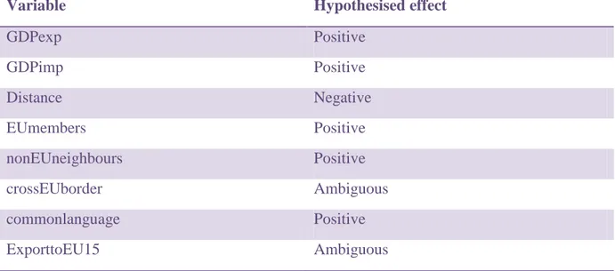
Table 5.1 Summary of hypotheses.

Variable Hypothesised effect

GDPexp Positive GDPimp Positive Distance Negative EUmembers Positive nonEUneighbours Positive crossEUborder Ambiguous commonlanguage Positive ExporttoEU15 Ambiguous

5.2

Other Assumptions and Information

Except from the variable specific information and assumptions, as presented in Chapter 5.1, there are additional information and assumptions that need to be disclosed.

For all variables where borders have been of importance, such as the nonEUneighbours and crossEUborder variables, the relationships have been based on land borders only. Countries being situated on opposite side of, for example, a strait or channel such as the UK and France are therefore not registered as neighbouring countries in the data.

Even though the period examined is from 1995 to 2006 all 46 countries are not included for all years. This is due to the data availability in Comtrade. In 1995 only 39 out of the total sample of countries were available. In 1996 data on Albania, Bulgaria, the Russian Federation and Ukraine became available thereby increasing the sample to 43 countries. Belarus entered the dataset in 1998 and lastly Belgium and Luxembourg entered in 1999 since the earlier data combined the two countries into one export value. One could have included the combined value prior to 1999 if it did not complicate the distance measure, since they have one capital each. In addition it would be difficult to properly state official languages and common borders.

21

5.3

Econometric model

To estimate the regression model the ordinary least squares method (OLS) is used on cross-sectional data for all the years included in the sample. An alternative method applicable for this data, as suggested by Gujarati (2003) is to pool the data into a least square dummy variable method (LSDV) so that one regression can be estimated instead of several ones; 13 in this case. However, the first method described suites the purpose of this study better by showing how all the coefficients change over the years, instead of showing whether a year is higher or lower on the whole than the base year.

After conducting White’s General Heteroscedasticity Test it became evident that the there was heteroscedasticity present in the data. There could be several reasons for that which is applicable on the dataset used in this study. Firstly, there are many countries of various economic sizes present and one cannot expect the variance in export value to be the same for e.g. the USA and FYR Macedonia considering the large difference in their GDP values. As explained by Gujarati (2003, p.401) “in cross-sectional data involving heterogeneous units, heteroscedasticity may be the rule rather than the exception”. Secondly, including many dummy variables in a model is always combined with an increasing risk for heteroscedasticity problems since one cannot expect the variance to be equal for the group where the dummy is 1 and the group where it is 0 (Aczel & Sounderpandian, 2006).

Having heteroscedasticity present in the data makes the estimators inefficient, the variances are under- or overestimated and therefore the regression results may be misleading (Gujarati, 2003). To remedy this problem the White’s heteroscedasticity-consistent standard errors are computed and presented instead of the regular standard errors.

5.4

Descriptive Statistics

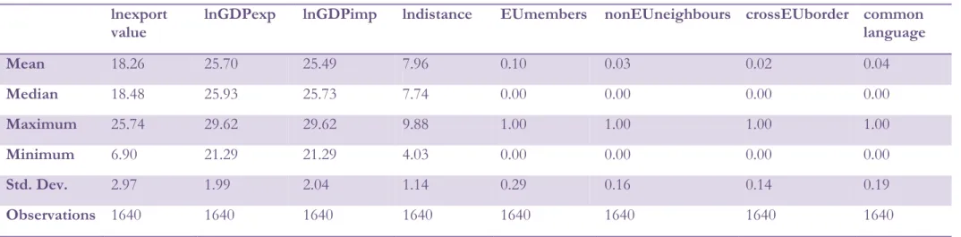
The descriptive statistics for the first and the last year of the sample are found in Table 5.2., and Table 5.3., below. Looking at the first variable, the lnexportvalue, many interesting things are discovered. Firstly, the median has increased more than the mean, suggesting that the central point in the dataset has increased more than the average value. This could be interpreted as an indicator that more bilateral flows have high values in 2006 than in 1995. This is also consistent with the second observation; that the range of export values has increased over the years. However, at the same time the standard deviation is almost constant. This means that the average distance from the mean is about the same although the range of possible values has increased, which suggests that most values have converged in the middle. For the GDP-values of the exporter it is apparent that the standard deviation has decreased together with the range in 2006 compared to 1995. This suggests that the countries in the sample have been converging over the years and the same trend is seen for the importing countries’ GDP-values. The mean and median in 2006 are more or less the same for the exporting countries and the importing countries. This was not the case in 1995 where the exporting countries had higher GDP than the importing countries according to the mean and median values. Thus it seems that rich countries exported to relatively poor countries in 1995 compared to 2006. Another way to interpret this development is to say that the countries that were relatively poor in 1995 have caught up with their relatively rich trading partners in 2006.

22 Table 5.2 Descriptive statistics 1995.

lnexport

value lnGDPexp lnGDPimp lndistance EUmembers nonEUneighbours crossEUborder common language

Mean 18.26 25.70 25.49 7.96 0.10 0.03 0.02 0.04 Median 18.48 25.93 25.73 7.74 0.00 0.00 0.00 0.00 Maximum 25.74 29.62 29.62 9.88 1.00 1.00 1.00 1.00 Minimum 6.90 21.29 21.29 4.03 0.00 0.00 0.00 0.00 Std. Dev. 2.97 1.99 2.04 1.14 0.29 0.16 0.14 0.19 Observations 1640 1640 1640 1640 1640 1640 1640 1640

Table 5.3 Descriptive statistics 2006. lnexport

value

lnGDPexp lnGDPimp lndistance EUmembers nonEUneighbours crossEUborder common language Mean 19.31 26.20 26.19 7.88 0.24 0.01 0.02 0.04 Median 19.68 26.50 26.50 7.63 0.00 0.00 0.00 0.00 Maximum 26.48 30.20 30.20 9.88 1.00 1.00 1.00 1.00 Minimum 2.30 21.95 21.95 4.03 0.00 0.00 0.00 0.00 Std. Dev. 2.95 1.84 1.85 1.13 0.43 0.12 0.15 0.20 Observations 2058 2058 2058 2058 2058 2058 2058 2058