Linköpings universitet SE–581 83 Linköping
Linköping University | Department of Computer and Information Science
Master thesis, 30 ECTS | Software Engineering
202019 | LIU-IDA/LIU-IDA/LITH-EX-A–18/054–SE-EX-A--2019/001--SE
Comparison of Auto-Scaling
Poli-cies Using Docker Swarm
Jämförelse av autoskalningpolicies med hjälp av Docker Swarm
Henrik Adolfsson
Supervisor : Vengatanathan Krishnamoorthi Examiner : Niklas Carlsson
Upphovsrä
De a dokument hålls llgängligt på Internet – eller dess fram da ersä are – under 25 år från pub-liceringsdatum under förutsä ning a inga extraordinära omständigheter uppstår. Tillgång ll doku-mentet innebär llstånd för var och en a läsa, ladda ner, skriva ut enstaka kopior för enskilt bruk och a använda det oförändrat för ickekommersiell forskning och för undervisning. Överföring av upphovsrä en vid en senare dpunkt kan inte upphäva de a llstånd. All annan användning av doku-mentet kräver upphovsmannens medgivande. För a garantera äktheten, säkerheten och llgäng-ligheten finns lösningar av teknisk och administra v art. Upphovsmannens ideella rä innefa ar rä a bli nämnd som upphovsman i den omfa ning som god sed kräver vid användning av dokumentet på ovan beskrivna sä samt skydd mot a dokumentet ändras eller presenteras i sådan form eller i så-dant sammanhang som är kränkande för upphovsmannens li erära eller konstnärliga anseende eller egenart. För y erligare informa on om Linköping University Electronic Press se förlagets hemsida h p://www.ep.liu.se/.
Copyright
The publishers will keep this document online on the Internet – or its possible replacement – for a period of 25 years star ng from the date of publica on barring excep onal circumstances. The online availability of the document implies permanent permission for anyone to read, to download, or to print out single copies for his/hers own use and to use it unchanged for non-commercial research and educa onal purpose. Subsequent transfers of copyright cannot revoke this permission. All other uses of the document are condi onal upon the consent of the copyright owner. The publisher has taken technical and administra ve measures to assure authen city, security and accessibility. According to intellectual property law the author has the right to be men oned when his/her work is accessed as described above and to be protected against infringement. For addi onal informa on about the Linköping University Electronic Press and its procedures for publica on and for assurance of document integrity, please refer to its www home page: h p://www.ep.liu.se/.
Abstract
When deploying software engineering applications in the cloud there are two similar soft-ware components used. These are Virtual Machines and Containers. In recent years containers have seen an increase in popularity and usage, in part because of tools such as Docker and Kubernetes. Virtual Machines (VM) have also seen an increase in usage as more companies move to solutions in the cloud with services like Amazon Web Services, Google Compute Engine, Microsoft Azure and DigitalOcean. There are also some solu-tions using auto-scaling, a technique where VMs are commisioned and deployed to as load increases in order to increase application performace. As the application load decreases VMs are decommisioned to reduce costs.
In this thesis we implement and evaluate auto-scaling policies that use both Virtual Ma-chines and Containers. We compare four different policies, including two baseline policies. For the non-baseline policies we define a policy where we use a single Container for every Virtual Machine and a policy where we use several Containers per Virtual Machine. To compare the policies we deploy an image serving application and run workloads to test them. We find that the choice of deployment strategy and policy matters for response time and error rate. We also find that deploying applications as described in the method is estimated to take roughly 2 to 3 minutes.
Acknowledgments
I want to thank my family and my beloved Sofia for helping me through this thesis. I also want to thank Niklas Carlsson and Johan Åberg for providing guidance and help with writing the thesis, as well as Raymond Leow for being my opponent and giving me great feedback. I also want to thank Sara Berg for reading my thesis and providing me with great feedback.
Contents
Abstract iii
Acknowledgments iv
Contents v
List of Figures vii
List of Tables x Listings xi 1 Introduction 2 1.1 Motivation . . . 2 1.2 Aim . . . 3 1.3 Research Questions . . . 3 1.4 Delimitations . . . 3 2 Background 4 2.1 Briteback . . . 4 3 Theory 5 3.1 Microservice Architecture . . . 5 3.2 Virtualization . . . 6 3.3 Elasticity . . . 10 3.4 Measuring Elasticity . . . 11 3.5 Taxonomy . . . 12 3.6 Cloud Computing . . . 15 3.7 Control Theory . . . 16 3.8 Related Work . . . 16 4 Method 19 4.1 Sending Requests . . . 19 4.2 Image Server . . . 21 4.3 DigitalOcean Evaluation . . . 21 4.4 Policy Experiments . . . 23 4.5 Auto-Scaling Implementation . . . 25 5 Results 30 5.1 DigitalOcean Evaluation . . . 30
5.2 Download Times for Docker Image . . . 31
5.3 Optimal Number of Containers for Mixed Policy . . . 32
5.4 Startup and Shutdown Times for Containers . . . 33
5.6 Policy Experiments for Baseline and Comparison . . . 43
6 Discussion 54 6.1 Results . . . 54
6.2 Method . . . 55
6.3 Source Criticism . . . 57
6.4 The Work in a Wider Context . . . 58
7 Conclusion 59 7.1 Discussion of Future Work . . . 60
A Early Deployment Figures 61
List of Figures
3.1 Microservices are built around single components that provide a standalone service,
while monoliths are centralized systems. . . 6
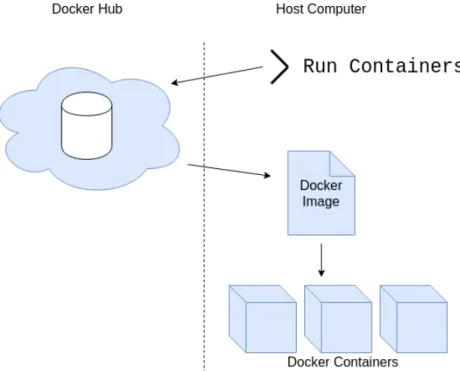
3.2 A Docker command is issued to run containers on the local computer. Docker then downloads an image from Docker Hub, the repository of Docker Images, and then runs a set of containers from the Docker Image specification. . . 8
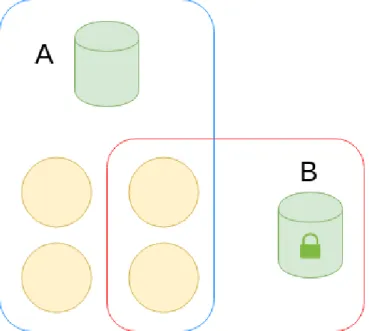
3.3 An example with Docker Compose service definition. A is a network that connects all four services to a common database. B is a network that connects a subset of services to the trusted store. . . 9
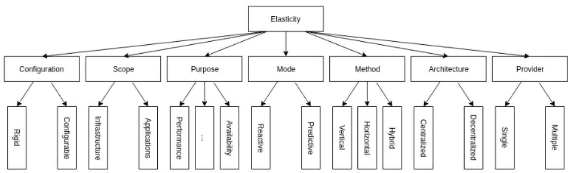
3.4 Horizontal and vertical elasticity. Vertical means scaling individual capabilities of computing resources and horizontal means scaling the number of computing resources. 10 3.5 A simplified image of the taxonomy of elastic systems described by Al-Dhuraibi et al. . . 15
3.6 Feedback controller of ElastMan . . . 17
3.7 Feedforward controller of ElastMan . . . 17
4.1 Exponentially rising in a few small steps. . . 20
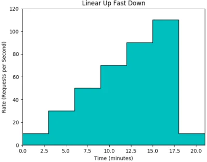
4.2 Linearily increasing the rate of accesses until dropping of at the end to the starting intensity. . . 20
4.3 Traffic is increased to an order of magnitude more in an instant. This continues for 15 minutes until it goes back to its starting value. . . 21
4.4 The image that was used during the auto-scaling experiment. . . 21
4.5 The test program that tested startup time for VMs on DigitalOcean. . . 22
4.6 The test program that tested shutdown time for VMs on DigitalOcean. . . 22
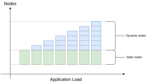
4.7 Expected scaling behaviour of the application . . . 26
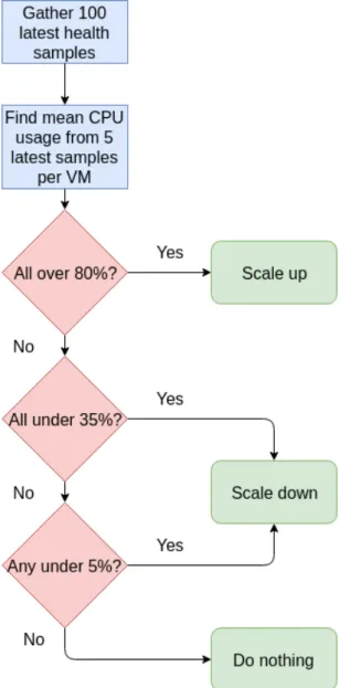
4.8 The algorithm used by the scaling decider. How it scales up or down depends on the currently active policy. . . 27
4.9 The classification of the system, using the taxonomy developed by Al-Dhuraibi et al. The blue colored boxes represent the classification of the system. . . 29
5.1 On the left: The CCDF of startup times for VMs on DigitalOcean. On the right: The same data but plotted on a logarithmic scale. . . 30
5.2 On the left: The CCDF of shutdown times for VMs on DigitalOcean. On the right: The same data but plotted on a logarithmic scale. . . 31
5.3 On the left: the CCDF for download times when downloading the image server Docker Image. On the right: The CCDF for download times when downloading the image server Docker Image, plotted using a logarithmic scale on the Y-axis. . . 32
5.4 The actual response time for each container setup. . . 32
5.5 The response time for each container setup as relative to the minimum response time for that column in the graph. Datapoints for 1 container is not visible for 100 and 120 requests per second. Datapoint for 2 containers is not visible for 120 requests per second. . . 33
5.6 The figure shows the time it takes for the containers to scale from 0 replicas to N replicas on a single node. The orange line is the median, the box shows the 95% range, the whiskers show the 99% range and the black circles shows the rest 1%. . 34 5.7 The figure shows the time it takes for the containers to scale from N replicas to 0
replicas on a single node. The orange line is the median, the box shows the 95% range, the whiskers show the 99% range and the black circles shows the rest 1%. . 35 5.8 The figure shows the time it takes for the containers to scale from N-1 replicas to
N replicas on a single node. The orange line is the median, the box shows the 95% range, the whiskers show the 99% range and the black circles shows the rest 1%. . 35 5.9 The figure shows the time it takes for the containers to scale from N replicas to N-1
replicas on a single node. The orange line is the median, the box shows the 95% range, the whiskers show the 99% range and the black circles shows the rest 1%. . 36 5.10 The results of the VM Only policy with the Exponential Ramp workload. The top
graph shows the number of VMs and the error rate. The middle graph shows the request rate as well as the maximum, average and minimum request time. The bottom graph shows the distribution of containers over different nodes. . . 38 5.11 The results of the VM Only policy with the Linear Rise, Fast Drop workload. The
top graph shows the number of VMs and the error rate. The middle graph shows the request rate as well as the maximum, average and minimum request time. The bottom graph shows the distribution of containers over different nodes. . . 39 5.12 The results of the VM Only policy with the Instant Traffic workload. The top
graph shows the number of VMs and the error rate. The middle graph shows the request rate as well as the maximum, average and minimum request time. The bottom graph shows the distribution of containers over different nodes. . . 40 5.13 The results of the Mixed policy with the Exponential Ramp workload. The top
graph shows the number of VMs and the error rate. The middle graph shows the request rate as well as the maximum, average and minimum request time. The bottom graph shows the distribution of containers over different nodes. . . 41 5.14 The results of the Mixed policy with the Instant Traffic workload. The top graph
shows the number of VMs and the error rate. The middle graph shows the request rate as well as the maximum, average and minimum request time. The bottom graph shows the distribution of containers over different nodes. . . 42 5.15 The results of the Mixed policy with the Linear Rise, Fast Drop workload. The
top graph shows the number of VMs and the error rate. The middle graph shows the request rate as well as the maximum, average and minimum request time. The bottom graph shows the distribution of containers over different nodes. . . 43 5.16 The result of the Constant policy on a small VM with the Exponential Ramp
workload. The middle graph shows the request rate as well as the maximum, average and minimum request time. The bottom graph shows the distribution of containers over different nodes. . . 44 5.17 The result of the Constant policy on a big VM with the Exponential Ramp
work-load. The middle graph shows the request rate as well as the maximum, average and minimum request time. The bottom graph shows the distribution of containers over different nodes. . . 45 5.18 The result of the VM Only policy on a small VM with the Exponential Ramp
workload and late deployment policy. The middle graph shows the request rate as well as the maximum, average and minimum request time. The bottom graph shows the distribution of containers over different nodes. . . 46 5.19 The result of the VM Only policy on a big VM with the Exponential Ramp workload
and late deployment policy. The middle graph shows the request rate as well as the maximum, average and minimum request time. The bottom graph shows the distribution of containers over different nodes. . . 47
5.20 The result of the Mixed policy on a small VM with the Exponential Ramp workload and late deployment policy. The middle graph shows the request rate as well as the maximum, average and minimum request time. The bottom graph shows the distribution of containers over different nodes. . . 48 5.21 The result of the Mixed policy on a big VM with the Exponential Ramp workload
and late deployment policy. The middle graph shows the request rate as well as the maximum, average and minimum request time. The bottom graph shows the distribution of containers over different nodes. . . 49 5.22 The result of the Container Only policy on a small VM with the Exponential Ramp
workload. The middle graph shows the request rate as well as the maximum, average and minimum request time. The bottom graph shows the distribution of containers over different nodes. . . 50 5.23 The result of the Container Only policy on a big VM with the Exponential Ramp
workload. The middle graph shows the request rate as well as the maximum, average and minimum request time. The bottom graph shows the distribution of containers over different nodes. . . 51 5.24 The result of the Mixed policy on a small VM with the Exponential Ramp workload
using the early deployment strategy. The middle graph shows the request rate as well as the maximum, average and minimum request time. The bottom graph shows the distribution of containers over different nodes. . . 52 5.25 The result of the VM Only policy on a big VM with the Exponential Ramp workload
using the early deployment strategy. The middle graph shows the request rate as well as the maximum, average and minimum request time. The bottom graph shows the distribution of containers over different nodes. . . 53 A.1 The result of the VM Only policy on a small VM with the Exponential Ramp
workload using the early deployment strategy. The middle graph shows the request rate as well as the maximum, average and minimum request time. The bottom graph shows the distribution of containers over different nodes. . . 61 A.2 The result of the Mixed policy on a big VM with the Exponential Ramp workload
using the early deployment strategy. The middle graph shows the request rate as well as the maximum, average and minimum request time. The bottom graph shows the distribution of containers over different nodes. . . 62
List of Tables
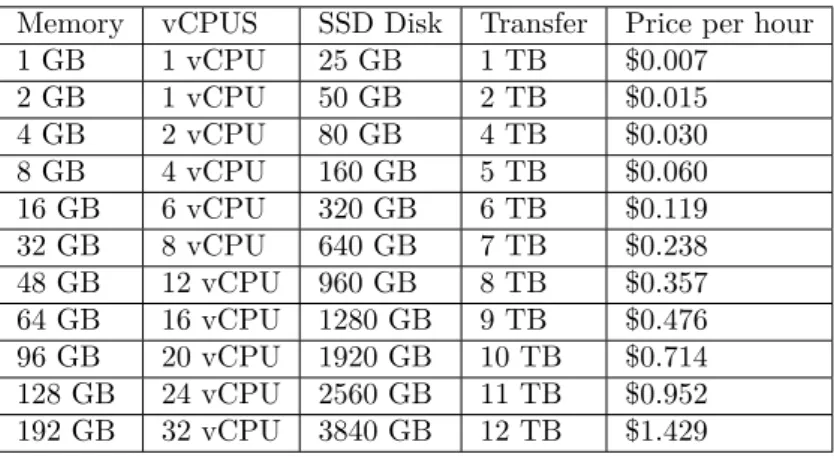
4.1 Scaling configuration for different scaling policies. . . 24 4.2 Standard Droplets offered by DigitalOcean . . . 28 5.1 Average request times for 1, 2, 3, ..., 10 containers with request times between 5
and 120 per second. Each row is a separate container count and each column is a separate request-per-second count. . . 33 5.2 Error rate and price for VM Only and Mixed policy. . . 37
Listings
3.1 An example “Dockerfile” that creates an application extended from the Ubuntu image and puts the application in /app, exposes port 80 (uses port 80 on the host and sends anything on that port to the container). Lastly when the image is run as a container it will run the run-script.sh with “start” as the first command line argument. . . 7 3.2 An example Docker Compose File (version 3) that creates a single service,
host-ing a service called “rethink”. The Docker Image used is called “rethinkdb” and the ports 29015, 28015 and 8080 are used by the image. Additionally, /root/rethinkdb on the host is mapped to /data in the container . . . 8
Glossary
This chapter lists different shortings or shorthands used in the text.
• API - Application Programming Interface. Interface for working with an application programmatically
• AWS Lambda - Amazon Web Services Lambda, An Amazon hosting service • CLI - Command Line Interface
• CTMC - Continuous-Time Markov Chain • EC2 - Amazon Elastic Compute Cloud
• NIST - National Institute of Standards and Technology
• PaaS - Platform as a Service (Amazon EC2, DigitalOcean, etc.) • SLO - Service Level Objective
1
Introduction
The introduction will mention a brief background into the area of cloud computing. It will also mention some results of previous research and the main motivation for studying this particular area of research. Then it will discuss the aim of the thesis, list the research questions and end the chapter with delimitations on the main work of the thesis.
1.1 Motivation
A new type of service has caught the eye of researchers and the IT industry in recent years. The service is called Platform as a Service (PaaS) and allows for renting compute capabilities in the cloud. Providers of these services are called Cloud Hosting Providers. This service allows customers to rent servers without having to tackle problems such as server uptime, component failure and hosting space. Companies like Amazon, Google, Microsoft, RedHat and DigitalOcean offer PaaS with different paid plans for different use cases. Previous research have shown that using a cloud computing solution provides benefits in form of: lowering cost, maintaining high resource utilization and being able to accommodate for a sudden burst in usage [1].
A common software architecture pattern used with hosting providers is the microservice ar-chitecture. It is a pattern in which services are split into different independent specialized servers, often smaller in size compared to using a single server. When hosting these servers in the cloud it is possible to allocate more or less resources to each individual VM that the server runs on. The providers often have different price plans for different types of VMs and the providers allow the type to be changed while applications are running. Changing the VM configuration can be done programmatically through an API, adding more VMs or removing VMs , and this creates an interesting research opportunity. Cloud hosting providers allow for users of their service to both monitor activity and react to it automatically and this can be used to create tools for automatic scaling, also known as auto-scaling. It has been shown that taking user performance requirements and economic factors into consideration in the scaling mechanism can reduce the cost in a cloud computing environment [2].
Studying the problem of scaling with dynamic resources has both academic purpose and eco-nomic purpose. As an academic it is interesting to understand good strategies of analyzing
1.2. Aim
activity and then scaling accordingly. It is a complex and non-trivial area of study, as it may depend heavily on context. Nevertheless, this makes it interesting to study independent of the context it is studied in. We can compare this perspective to that of a business. As a business it is important to be profitable and deliver a good service. The scaling of the servers will directly relate to both the quality of the service and the cost of running the service. Thus, for a business, it is interesting to study this problem because it allows the business to scale their servers in a cost-conscious way.
There have been several attempts to find good algorithms and techniques to achieve good auto-scaling [3]. There are two major groups for auto-auto-scaling techniques: proactive and reactive. A proactive algorithm tries to predict the future from historical data while a reactive algorithm reacts to workload or resource utilization according to a set of predefined rules and thresholds in real-time [4]. This thesis studies the effects of Container based scaling and Virtual Machine based scaling using part of a real world application.
1.2 Aim
This thesis aims to compare auto-scaling policies using part of an application built with a microservice architecture. The different policies for scaling differs in the number of containers and virtual machines they spawn.
1.3 Research Questions
• How does an auto-scaling policy based on static thresholds compare when scaling with different policies, in regards to container and/or virtual machines, when it comes to cost and SLO violations?
1.4 Delimitations
The thesis will focus on what is possible to achieve with DigitalOcean and Docker Swarm. Docker is a common tool for defining software containers and Docker Swarm is a tool for creating and managing a fleet of containers. DigitalOcean is a cloud hosting provider that allows users to rent VMs.
2
Background
This chapter describes important parts of the context for the study that is part of the thesis.
2.1 Briteback
The company that the experiments were performed at is called Briteback. Their main prod-uct is a communication platform for larger companies, realized as an application for several different platforms. Part of this application is used in the experiments, and so it is important that it is explained in sufficient detail.
Briteback has built their main application using microservices, meaning that they have many different types of services that run independently. One of the services used in the Briteback application is the image service. This service is used to download, crop and scale images that are later displayed in the application. This service will be the target of the auto-scaling experiment of this thesis. All of Britebacks services are created using a tool called Docker and they are deployed on a hosting provider called DigitalOcean. Docker is a tool for creating and running containers.
This study will be used by Briteback as groundwork for investigating an auto-scaling solution for the production environment of the company.
3
Theory
This chapter explains different concepts needed to understand how the method was formed and realized.
3.1 Microservice Architecture
Software can follow different types of high level architectural designs. Within web development it is common to talk about monolithic and microservice architectures. They are commonly contrasted with each other because of their definitions. The National Institute of Standards and Technology (NIST) defines microservices in the following way[5]:
Microservice: A microservice is a basic element that results from the
archi-tectural decomposition of an application’s components into loosely coupled patterns consisting of self contained services that communicate with each other using a stan-dard communications protocol and a set of well defined API’s, independent of any vendor, product or technology.
NIST defines a microservice as a part of a bigger application. The individual service has to be able to work, mostly, on its own. It needs to be connected with other microservices that together form the application, as visible to the end user.
The definition given by NIST fits well with the domain. The individual servers are of varying sizes and each is characterized by its available interface (API) as well as the human-defined “aim” of the server. The definition also fits well with other research in the area, such as the definitions given by Dragoni et al. [6].
Monolithic applications, as opposed to microservices, are applications in which there is only one server managing the application. Even tough “monolithic” usually has negative connotations from a programming perspective it is important to understand that a monolithic application is not, by definition, worse than a microservice architecture. Instead it has different benefits, drawbacks and challenges compared to a microservice architecture.
In comparing monolithic and microservice applications there is research that suggests microser-vices cost less when deployed in the cloud. Villamizar et al. found that they could reduce
3.2. Virtualization
infrastructure costs by up to 77% when deploying an application through AWS Lambda, when comparing an application written with both a monolithic and microservice architecture [7]. Dragoni et al. [6] also argue that a microservice architecture help in many modern software engineering related practices. Having a service with well-defined barriers help programmers find bugs faster. Having several smaller services is ideal for containerization and thus improves portability and security. Scaling several smaller servers allows for fine-tuning of the scaling and can save costs, rather than increasing the capability of every service which a monolith has to do [6].
A conceptual image of what a microservice architecture looks like can be seen in Figure 3.1. The figure depicts a monolith architecture and a microservice architecture. The monolith has all software components communicating with each other and access to the same database. In the microservice architecture each software component has their own (smaller) database and can run fully independently. However, they need to communicate with other microservices over the network using a standard protocol, such as HTTP.
Figure 3.1: Microservices are built around single components that provide a standalone service, while monoliths are centralized systems.
ECMAScript and Node
The microservices that are examined as part of the thesis are written in the programming language ECMAScript, more commonly refered to as JavaScript. These run as servers with the help of Node.js, a runtime environment for JavaScript. Node is built on the V8 JavaScript engine found in Google Chrome [8]. It is a programming environment heavily focused on asynchronous programming and non-blocking I/O. This makes it suitable as a runtime for creating a scalable system [9]. Programming in JavaScript with Node suits both a monolithic approach as well as a microservice approach.
3.2 Virtualization
Virtualization is a concept used in computing that means abstracting away from the underlying architecture. Virtualization is used to sandbox different environments. A common use-case is to run a Virtual Machine (VM) with a different Operating System (OS) than that of the original machine. This allows for running a Linux machine inside of a Windows machine and vice versa. To refer to the actual machine running the virtualization environment we use the word “host” and to refer to the VM that runs we use “guest” and say that the guest machine(s) runs on the host. Intuitively, a virtualized environment should run slower, compared to running on the host environment. While this is mostly correct, there are virtualization tools that run with very little overhead [10].
3.2. Virtualization
Apart from virtual machines there is also a technique called containerization. Instead of using virtual machines you use “containers”. A key difference being that a VM runs on virtual hardware with its own kernel while a container runs the same OS as the host and only has limited access to the host. Containers run faster compared to using a VM and also start faster [11]. There is also research suggesting that the difference between containers and running code directly on the host is negligible [12].
Virtualization has properties that are useful to software applications. In this section we men-tion some of the benefits and describe them briefly.
Portability: An application defined inside of a virtualized environment can run anywhere the
virtualized environment can run. This property becomes very useful when an application is hosted in the cloud, on hardware provided by someone else [13].
Security: Applications deployed inside a virtualized environment typically cannot access the
host. Because of the sandboxed environment an attacker typically has to compromise the application and then escape the (restricted) virtualized environment to compromise the host [13].
Reliability: With virtual machines and containerization the running environment can be
treated as software, instead of being part of the hardware. A failure is then only a soft-ware failure and not a hardsoft-ware failure. This makes restarting the virtualized environment a valid fallback tactic for crashes, which is much harder to realize when actual hardware fails [13].
Docker
Docker is used to create software containers. It uses a scripting language to define what is called an image. The image defines what should exist in a container, if it should extend from a previous image and how it should be configured. From this image the Command Line Interface (CLI) can spawn containers and once spawned the CLI can access the containers and provide changes to the running environment or run programs in it. Docker also has a repository of shared images that can be used and extended upon, similar to open source communities such as GitHub [13]. It is called Docker Hub. Figure 3.2 shows a conceptual image of how running Docker containers on a single computer works. An example of an image definition is found in Listing 3.1.
Docker can also run in a mode called swarm mode, or Docker Swarm. It allows for managing a set of containers each providing its own service, as well as running duplicates of services for redundancy. Built into Docker Swarm are features commonly used when deploying applica-tions, such as load balancing and automatic failover [14]. Docker Swarm acts as a deployment agent, starting and stopping containers when it is told to. It decides where containers will run, when they will start, and when to restart containers that have failed or crashed. It uses the same API as the Docker CLI does, meaning that starting new containers work in the same way as when a human would start a container through Docker CLI, like depicted in Figure 3.2.
1 FROM ubuntu
2 CWD /app
3 COPY my− a p p l i c a t i o n / s r c /app/ s r c
4 COPY my− a p p l i c a t i o n /run− s c r i p t . sh /app/run− s c r i p t . sh
5 EXPOSE 80
6 ENTRYPOINT [ ” / app/ run− s c r i p t . sh ” , ” s t a r t ” ]
Listing 3.1: An example “Dockerfile” that creates an application extended from the Ubuntu image and puts the application in /app, exposes port 80 (uses port 80 on the host and sends
3.2. Virtualization
Figure 3.2: A Docker command is issued to run containers on the local computer. Docker then downloads an image from Docker Hub, the repository of Docker Images, and then runs a set of containers from the Docker Image specification.
anything on that port to the container). Lastly when the image is run as a container it will run the run-script.sh with “start” as the first command line argument.
For this thesis we use Docker to build an application image. Generally, an image would be built for each microservice. Images can also be less specific, for example a web server or a database. The setup, which utilize swarm mode, is defined through a Docker Compose File. This is a file following the YAML data standard and it defines a number of services run by Docker Swarm. Each service is based on an image, which in this case corresponds to the application images. Each service also has a number of properties that can be specified through the compose file, such as environment variables, container replicas, volumes, constraints and networks [15]. An example of a Docker Compose File can be seen in Listing 3.2.
1 v e r s i o n : ”3” 2 s e r v i c e s : 3 r e t h i n k : 4 image : r e t h i n k d b 5 p o r t s : 6 − ”29015” 7 − ”28015” 8 − ”8080” 9 volumes :
10 − / root / rethinkdb : / data
Listing 3.2: An example Docker Compose File (version 3) that creates a single service, hosting a service called “rethink”. The Docker Image used is called “rethinkdb” and the ports 29015, 28015 and 8080 are used by the image. Additionally, /root/rethinkdb on the host is mapped to /data in the container
3.2. Virtualization
Docker allows Compose Files to define volumes, directories mounted inside the container. A container can save data to the host by saving it in the given volume. It also works in the reverse direction. A host can save data to a volume in order for the container to read information. Volumes are a common way of giving access to company secrets inside a container. Secrets would be data, such as SSH keys or authentication tokens. Images are stored in the cloud and thus you do not want to store your secret inside the image, as anyone with the image can run the container [15].
In a Compose File it is also possible to define constraints, when working in swarm mode. Con-straints are general conCon-straints on where to run a service. For example, running a database on the weakest of four nodes may hamper application performance if the database is a bottleneck. Or perhaps the application is CPU intensive and it is important to run the CPU intensive tasks on the node with the most CPU’s. This can be achieved with constraints by specifying that a service needs a minimal amount of CPU/memory or specify a node that it runs on. Labels can manually be added to nodes through the Docker CLI and constraints can specify labels that they run on [15].
Compose Files allow for custom networks to be defined as well. These are networks that join services together. For example an application may have a database which every other service needs to be able to connect to but it also has a trusted store, which sensitive information is kept in, that can only be accessed by a few of the other services. In that case it would be possible to create two different networks, one with the database and one with the trusted store. In the Compose File you would then specify that the services with permission to access the trusted store is part of the same network as the trusted store [15]. This scenario is depicted in Figure 3.3.
Figure 3.3: An example with Docker Compose service definition. A is a network that connects all four services to a common database. B is a network that connects a subset of services to the trusted store.
In order to run the configurations in a Compose File you can deploy it to a Docker Swarm. The swarm will then try to deploy all the containers in a way that satisfies the constraints and requirements of the Compose File. The file can be updated and redeployed and the swarm will try to update the running services in the swarm. It is also possible to manually update parameters of the compose file, for example scaling the number of container replicas for a single service [14].
3.3. Elasticity
Figure 3.4: Horizontal and vertical elasticity. Vertical means scaling individual capabilities of computing resources and horizontal means scaling the number of computing resources.
3.3 Elasticity
There are many definitions of elasticity. Here we will list key elements of elasticity and compare the literature in the area.
Horizontal elasticity: Increase or decrease the number of computing resources. Vertical elasticity: Increase or decrease the capacity of available computing resources.
The definitions of horizontal and vertical elasticity are taken from Al-Dhuraibi et al. [4]. Hor-izontal elasticity and vertical elasticity are orthogonal concepts in nature and cloud providers can provide both at the same time. It is also possible to impose restrictions on how the scaling works. For example imposing restrictions on vertical elasticity to only work between comput-ing resources of the same priccomput-ing. Even though the verticality of the elasticity is constrained it would still be vertical elasticity. The concept of vertical and horizontal elasticity is shown in Figure 3.4.
Over-provisioning: auto-scaling that has resulted in having a higher supply of processing power
than demand.
Under-provisioning: auto-scaling that has resulted in having a higher demand than available
processing power.
These two definitions are given by Al-Dhuraibi et al. [4]. This is not the only definition of Over-provisioning and Under-Over-provisioning. Ai et al. [16] define three states of the system instead of two. Apart from the above it defines the Just-in-Need state [16]. This state is supposed to capture when the application runs at optimal scale, the supply matches the demand closely. However, an issue with the definitions of Ai et al. [16] is how the states are derived from the number of requests to the system and the number of VMs the system has available. The Just-in-Need state is defined as a⋅i < j ≤ b⋅i where i is the number of requests, j is the number of available VMs and a and b are constants such that a< b. In the paper they specifically use the value 1 and 3 for a and b, respectively. These values are not justified but it is mentioned that they will need to be modified depending on the cloud platform and context.
3.4. Measuring Elasticity
Automation: The degree of which the system is able to scale without interaction from
some-thing that is not part of the system.
Optimization: The degree of optimization for the application run by the system.
The above definitions are used by Al-Dhuraibi et al. to define and summarize elasticity [4]. Their paper defines elasticity as the combination of Scalability, Automation and Optimization. For elasticity you need auto-scaling, or you cannot handle an ever increasing workload, but an important part of the application is also the optimization of the application itself. If the application is not built to scale then it is hard to achieve an elastic application with only auto-scaling. Even tough there are limits to elastic provisions with inelastic of unoptimised programs, there is research suggesting non-elastic programs can become elastic with software tools for elastic configuration during runtime [17].
A lot of research has focused on a working implementation that utilizes some elastic concepts and exploring ways in which to achieve elasticity [1], [2], [16]–[30].
Elasticity Challenges
Elasticity is a large area, covering many different aspects of software engineering. The defini-tion by Al-Dhuraibi et al. [4] show that it covers not only the infrastructure that the system runs on, but on the code that is running as well. Roy et al. [23] list three main challenges for elastic resource provisioning with component-based systems. These are:
Workload Forecasting: By forecasting and predicting the workload it is possible to commision
computing resource just in time of need, instead of commisioning at the moment they are needed. The challenge becomes predicting when they are needed, forecasting how much stress the servers will be put under.
Identify Resource Requirements for Incoming Load: The system needs to be able to
accu-rately calculate the necessary resources for a load in order to avoid under-provisioning or over-provisioning.
Resource Allocation while Optimizing Multiple Cost Factors: A problem that occurs with the
overhead of resource provisioning is that it is impossible to follow the load exactly, which often fluctuates and can change drastically. Optimizing over such uncertainty and with the overhead constraints makes for a difficult problem to solve.
There is data suggesting the CPU-utilization is quite low for a lot of systems, with estimates around an average CPU-utilization of 15-20% [31].
3.4 Measuring Elasticity
An approach to measuring elasticity is defining the three states of over-provising, under-provisioning and just-in-need, as previously mentioned. The merits of this approach is that it is simple to create a metric, a comparable value, between two different solutions. The drawback is that the states are complex to define. Ai et al. [16] used this definition and created an elasticity value, representing the time a system is kept within the Just-in-Need state. They also tested their definition using a queueing model with a modified continuous-time Markov chain (CTMC). The CTMC modelled an underlying system and they tweaked values of the CTMC in order to see how the elasticity would be affected.
Ai et al. [16] prove, for their model, that it is a plausible model, mathematically. They also analyze the computed elasticity for different values of input variables, for example varying VM startup time. They also simulate their model using a simulator built in C++ and find that the simulation differs from the CTMC model with less than 1% difference. Apart from this
3.5. Taxonomy
they also run experimental tests and find that the experiments differs from their model with at most 3.0%.
Working with the elasticity definition presented by Ai et al. [16] has both positive and negative aspects. The positives are that it produces a comparable value between different algorithms and that the model developed by Ai et al. [16] is sound and tested mathematically, in sim-ulation and experimentally. However, it is not perfect. Part of the calcsim-ulations made by Ai et al. [16] is how the three different states are defined. The definitions, even though they are agnostic to the auto-scaling algorithm, may yield different results for different values. This implies that anyone using the elasticity value needs to make a subjective choice for how the states are defined. The paper, unfortunately, provides no guidance on how best to define the states. Apart from the definition of the states they also assume that the system to be scaled is centered around lending VMs to service requests, not requests to an application. The arguments in the paper are made from the perspective of a cloud service provider, but can be modified to be made from an application provider using a cloud service provider. The main issue then is that the states cannot be defined with the relatively low boundaries that Ai et al. [16] use, but would be defined with request sizes several orders of magnitude larger.
3.5 Taxonomy
For the purpose of this thesis we will use the taxonomy provided by Al-Dhuraibi et al. [4] They define seven different properties in order to classify an elastic system and in this section we briefly describe the taxonomy. It is divided into seven subsections, each describing a property found in the work of Al-Dhuraibi et al. [4] The taxonomy is summarized in Figure 3.5.
Configuration
Configuration is a property that looks at how computing resources are offered by a cloud provider. Two types of configuration are defined, rigid and configurable. A rigid configuration means that a customer can choose between different fixed types of computing resources. For example, DigitalOcean uses fixed instances where you buy nodes and each node has an hourly price. There are different types of nodes and each node has a specific number of virtual CPUs, a specific memory size and a specific bandwidth. A configurable configuration allows the customer to choose resources for a VM, for example the number of CPUs.
How resources are reserved is a property that falls under Configuration and Al-Dhuraibi et al. [4] define four standard ways of reserving resources as well as an “other” category. The categories are:
• On-demand reservation - Reservations are made as they are needed and result in either rejection of reservations or acceptance of reservations.
• In advance reservation - Reservations are made in advance of the necessary timeframe and are guaranteed to be available at the specified time.
• Best effort reservation - Reservations are queued and handled on a first-come-first-serve basis.
• Auction-based reservation - Reservations are made dynamically through bidding and will be made available as soon as the customer wins a bid.
Scope
Scope defines at what level, or which levels, scaling actions occur. For example scaling could occur inside an application, but it can also occur at infrastructure level. Al-Dhuraibi et al. [4]
3.5. Taxonomy
note that most of the elasticity solutions they examined provide solutions at the infrastructure level. An important concept to bring up before going into detail is the concept of sticky sessions. Sticky sessions mean that an application carries state, meaning that applications can be session based, and that sessions and their state needs to be preserved when performing scaling actions. An example would be an application which allows for video calls. If the application can scale with sticky sessions then video calls would not be interupted by the scaling mechanism, however if the scaling mechanism assumed a stateless application then the video call might suddenly end, or require complex client code to continue.
Al-Dhuraibi et al. [4] define the infrastructure level to have two main branches. One branch where containers are scaled and one where VMs are scaled. They also define embedded elas-ticity solutions, which are aware of the application in some way. Within embedded elaselas-ticity they define two subcategories, application map and code embedded. Code embedded is when the elasticity solution is part of the application itself. The application uses internal metrics to decide on how to scale. The drawback of this approach is that it needs to be tailored for each application as it is an integral part of the application. Application map is defined as an elasticity controller that has a complete view of the application, including the components of the application. Each component is either static or dynamic. Static components are launched at the start of the application execution and dynamic components are launched as part of the scaling [4].
Purpose
Elasticity has different purpose depending on the goal with the application and its execution. For example improving performance and reducing costs can be interesting for the ones deploy-ing an application while quality of service is important for the cloud provider. Al-Dhuraibi states that “elasticity solutions cannot fulfill the elasticity purposes from different perspectives at the same time”. For example one cannot seek to maximize performance while minimizing environmental footprint, as both cannot be achieved at the same time. However, purposes that are not contradictory can be combined, such as quality of service and performance [4]. The number of purposes for using an elastic systems are many but some of them are:
• Availability - Ensure that the application is available under increased/decreased work-loads.
• Energy - Minimize the amount of energy used by an application.
• Performance - Increase/decrease performance of an application under certain conditions. • Cost - Reduce the cost of the application.
• Capacity - Handle more users of the application simultaneously.
Mode
Mode defines how an application is scaled. An application can be scaled in three different ways. Automatically, manually or programmatically. In order for an application to be elastic it needs to scale automatically, the manual modes are not considered elastic. Manual mode means that a user has an interface provided by the cloud provider that allows them to scale their application. Programmable mode means that the application is scaled through API calls. Al-Dhuraibi claims that programmable mode is incompatible with elasticity, because it is the same as manual mode [4]. The reasoning is not clear because the focus is on the different subtypes of automatic mode and not elaborations on programmable mode.
Automatic mode can be divided into three main areas, each with their own approaches. The three areas are reactive, proactive and hybrid mode. Reactive means that the algorithm
3.5. Taxonomy
monitors events and tries to match supply with the demand of resources. Proactive means that the algorithm tries to analyze previous usage and detect patterns in demand, essentially predicting the demand for resources. Hybrid means that the solution uses a combination of the reactive and proactive approach to scale.
Reactive mode can be divided into two approaches, static and dynamic thresholds. Static thresholds means that elasticity actions are performed when measured metrics reach static thresholds. For example CPU utilization is above or below 50%. A lot of commercially available solution use this kind of metrics, such as Amazon EC2 and Kubernetes [32], [33]. Dynamic thresholds are also called adaptive thresholds because they adapt to the state of the hosted application.
Proactive mode can be divided into many approaches. Al-Dhuraibi shows five different ap-proaches. Each one of them is listed and briefly described below.
• Time series analysis - Use gathered metrics to try and predict future metrics. Perform elasticity actions based on comparing the predicted values to a set of thresholds and rules.
• Model solving mechanisms - Create a model of the application and find optimal rules for scaling using that model. An example model is Markov Decision Processes.
• Reinforcement learning - Create an agent that is responsible for scaling and receives rewards and punishments depending on the performance of the application.
• Control theory - Use a mathematical model and a controller (P-, PI-, PD- or PID-controller) to determine when to scale.
• Queueing theory - Use a mathematical model with waiting time, arrival rate and service time to model the system and make elasticity actions from that model.
It is important to note that some approaches can work both reactively and proactively. For example Al-Shistawy and Vlassov created an elasticity manager that uses control theory for both proactive and reactive decisions, resulting in a hybrid elasticity manager [29]. They reasoned that a reactive mode is good at handling unexpected workloads, such as unexpected flash crowds, while a proactive is good at handling long-term predictions, for example recurring flash crowds during mid-day.
Method
Method refers to which method is used to achieve elasticity. Al-Dhuraibi et al. [4] define two main approaches to this, horizontal and vertical elasticity, and state positives and negatives about the approaches. For this category there is also a possibility of a hybrid approach, but it is not further discussed.
Horizontal elasticity allows for new computing resources to be added. The drawback of hori-zontal elasticity is that it often works with very large increments of resources and fine-tuning the resources is not always possible. Vertical elasticity, while not being as available as hor-izontal, allows for fine-grained tuning of resources [4]. It is also important to note that the way an application is built makes a difference for what method is most appropriate. If the application is highly distributed, then it would likely work well with horizontal scaling, but if it has a lot of components that needs to communicate and are tightly interconnected, then it is likely that vertical elasticity would work better.
3.6. Cloud Computing
Figure 3.5: A simplified image of the taxonomy of elastic systems described by Al-Dhuraibi et al.
Architecture
The elasticity management solution can be architectured in one of two different ways. Ei-ther centralized or decentralized. A centralized architecture has one elasticity controller that makes elasticity scaling decisions while a decentralized one has several, independent ones. A decentralized elasticity manager also needs to have an arbiter component that is responsible for allocating resources to the controllers and the different system components [4].
Provider
This property denotes whether the elasticity manager uses a single or several cloud providers, if they are in different regions, different data centers etc.
3.6 Cloud Computing
There have been several attempts at defining cloud computing. NIST has provided a definition, just like they have with virtualization. NIST defines five properties that cloud computing must have [34]. These terms are listed and explained briefly:
• On-demand self service - A user of the service can automatically ask for up/downgraded service without human interaction.
• Broad network access - The provided service is available over the network over standard protocols. This allows any internet connected device to access it.
• Resource polling - Customers of the service are pooled together on the same machine. Additionally the physical location of the machine should not be apparent to the user but it can be visible on a higher level, such as region or country.
• Rapid elasticity - The service should allow for scaling the computational power provided to the user.
• Measured service - How the resources for a single user are used are both gathered and presented to the user.
Cloud computing is a necessary prerequisite for creating an auto-scaling mechanism and an elastic platform. The most important properties for elasticity and auto-scaling is On-demand self service as well as Rapid elasticity.
For cloud service providers it is also important to look at their cost models and their price models. Genaud et al. [25] has shown that it is possible with client-side provisioning, depending
3.7. Control Theory
on the pricing model, to optimise for different types of workloads . One of the key elements in their paper is that the cost model works in discrete increments of an hour, that is you pay for each started hour you rent. That way it is possible to fit several workloads within the same hour, while only paying for a single hour. They find that different strategies have different benefits and it is possible for a user to select a strategy based on their need.
3.7 Control Theory
Control theory is an area in which input signals are analyzed and output is generated from them. A widely used controller is the Proportional-Integral-Derivate (PID) controller. This controller continuously calculates the deviation from a desired reference signal r(t), or constant
r(t) = c, and adjusts the system based on the following formula: u(t) = KPe(t) + KI∫ t 0 e(T )dT + KD d dte(t). (3.1)
The above three terms corresponds to the proportional, integral, and derivative terms (P, I and D respectively) captures different aspects of these deviations. However, all three terms use the error signal e(t) at timepoint t. This signal can be calculated as e(t) = y(t)−r(t); the difference between the actual signal and the reference signal. The reference signal is a predefined signal defined by the one constructing the controller. KP, KI and KD are constants that are used
to change the behaviour of the controller. Constants can be zero and in that case they create a controller that is easier to analyze and work with [35].
Additional properties of a dynamic system that is being controlled by a controller are: • Stability - that the system settles for a final value with a constant reference signal • Robustness - that the properties of the system will be similar even if the underlying
mathematical model is not correct and
• Observability - that the system can observe all relevant state of the system.
On the Use of Control Theory for Auto-Scaling
A typical use of control theory is to handle and control flow of liquid to ensure that it flows at a certain rate. The usage of a network application can be viewed as a flow of network requests and the scaling of the cloud computing service can be viewed as a parameter to increase or decrease flow. The actual workings of the flow are complex and thus control theory is a natural fit for adapting to an increase or decrease in flow. By acquiring measurements, such as average response time, an auto-scaling solution can aim at a reference response time and scale accordingly.
Previous research in the field has established that using control theory for auto-scaling is a viable strategy. Serrano et al.[28] showed that Service Level Objectives (SLO) could be mapped to a utility function which can be used as input to a controller. They also showed that their implementation would be reactive to events and change the number of rented nodes, in order to meet SLOs. Lim et al. [36] showed that it was possible to use a discrete version of an integral controller in order to achieve auto-scaling, with regards to several different QoS measurements and SLOs.
3.8 Related Work
There is a lot of work in the area of cloud computing and especially regarding auto-scaling. Al-Dhurabi et al. [4] found that there are at least 15 different approaches to providing a
3.8. Related Work
Figure 3.6: Feedback controller of ElastMan
Figure 3.7: Feedforward controller of ElastMan
solution for the problem. One of the most common approaches was a threshold-based policy in which the service reacts against user defined rules in a ”If this then that” configuration. Marshall et al. [26] created such a system and tested it at Indiana University, University of Chicago and Amazon EC2. They created a tool in Python that allows system administrators to define their own policies for up-scaling and down-scaling. They also made an evaluation of the different hosting options they had chosen. The evaluation was done by sending a number of jobs to the server, each job sleeping for a certain amount of time. The study found that their solution could scale to over 150 nodes, it found that bootup times varied significantly and that termination of nodes was comparatively fast and consistent compared to bootup. Bootup times ranged between 74 and 205 seconds, while termination regularly took 3 to 4 seconds [26].
Al-Shistawy et al. [29] created a controller for auto-scaling a key-value store service. They called this system ElastMan. It consists of a feedback controller, a feedforward controller and an overarching program that decides between which controller to use. They create their controlling model from an SLO they call R99p, which means the read operation latency for the 99th percentile. They test the auto-scaling by sending it workloads with different intensities and show that their system can adjust to rapid changes in the environment, for example a flash crowd. They also show that using this approach costs less than using just a constant number of servers. The feedback controller is shown in Figure 3.6 and the feedforward controller is shown in Figure 3.7.
Vasić et al. [24] found that by analyzing the requests that come to a server and categorizing them allows for strategies that greatly increase adaptation speed, the time it takes for an elastic system to adapt to a new situation. They also show that a quick adaptation speed is correlated in monetary saving, in regards to service provisioning costs.
Sharma et al. [22] have investigated the effect of utilizing a cost model for defining the auto-scaling algorithm and take into account the usage based pricing models that are often used with resources provisioning. They managed to achieve a cost reduction of 24% in a private cloud setting and a 35% decrease on Amazon EC2. Their research suggests that in order to lower the cost of a system deployed in the cloud that uses elastic resource provisioning, the auto-scaling should have knowledge about the cost of provisioning.
Ashraf et al. [21] have created an approach for efficient auto-scaling called CRAMP (Cost-efficient Resource Allocation for Multiple web applications with Proactive scaling). It monitors resource utilization metrics of the infrastructure that the system runs on and does not need measurements from the application in order to achieve elasticity. It also uses shared hosting
3.8. Related Work
of applications, running them on the same VM, lowering the number of VMs required. By decoupling the applications from running on a single VM and scaling the underlying VM with information about resource utilization on the VMs they achieve significantly improved QoS for average response time and resource utilization. Ashraf et al. also created a user-admission system that was able to reduce server overload while simultaneously reducing rejected sessions [19].
Iqbal et al. [20] have shown that a strategy that uses both proactive and reactive scaling, a hybrid approach, is viable. Their system utilizes a reactive approach for scaling up and a proactive (predictive) approach for scaling down. Scaling up is based on the CPU usage while scaling down is based on an analytical model.
4
Method
In this chapter we present the method, including all the experiments we perform.
4.1 Sending Requests
During the experiment we will use a program that generates requests to the service and does so at a controlled rate. The program we will use is called Siege.1 It is a command line program
that can be invoked to create several “users” that will connect to a given URL. Siege is used for testing load capacity of a server. It also records important statistics when running, which is necessary for analyzing the performance of the application. Examples of these statistics are: minimum response time, maximum response time, average response time, number of failed requests and total number of connections. When running Siege it is possible to tell it to run with a certain number of users. Unfortunately there are no guarantees for the request intensity generated by Siege.
We define three different tests that all use a single workload each. The workloads are described below.
Workloads
Exponential Ramp - A workload that rises in intensity exponentially, after a set time doubles
in regular intervals, up to a threshold. The workload is described in Figure 4.1.
Linear Rise, Fast Drop - A workload that rises linearly, only to drop quickly. The workload is
described in Figure 4.2.
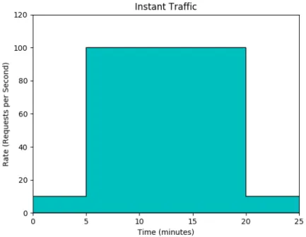
Instant Traffic - A workload that increase in a single step to an order of magnitude more in
intensity, from 10 requests per second to 100. The workload is described in Figure 4.3. The exact values to use for the size of workloads is not a trivial question. As described by Al-Dhuraibi et al [4], there is no standard method for evaluating the elasticity of a system. These workloads were chosen because they offer a variety of access patterns. They are also synthetic and are thus easy to use. Lastly, it was observed that the tested application reached a high
4.1. Sending Requests
Figure 4.1: Exponentially rising in a few small steps.
Figure 4.2: Linearily increasing the rate of accesses until dropping of at the end to the starting intensity.
level of CPU-utilization at around 40-50 requests per second for the big VM size. Because of this the workloads have a maximum request rate of double that.
4.2. Image Server
Figure 4.3: Traffic is increased to an order of magnitude more in an instant. This continues for 15 minutes until it goes back to its starting value.
4.2 Image Server
In order to isolate the scaling we will only use a small part of the Briteback application. We will be using a modified image server, which retrieves images from the web, stores them locally and performs cropping and scaling on images. We will use it in a mode that is CPU intensive, where the number of scaling operations on a container has been artificially inflated to create a bottleneck in CPU usage.
Siege is used to test the application and will send requests to fetch, crop and scale the image shown in Figure 4.4. This image is served by Linköpings University through the liu.se domain.
Figure 4.4: The image that was used during the auto-scaling experiment.
4.3 DigitalOcean Evaluation
In order to evaluate the startup and shutdown times of virtual machines we will run a perfor-mance evaluation of startup and shutdown times on DigitalOcean. These evaluations will use the small VM type.
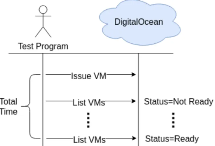
In order to test startup time we have developed a program that uses the DigitalOcean API in order to provision a virtual machine and measure the time until the machine is listed through the API as being ready. A similar program has been developed that decommisions the virtual machine and measures the shutdown time by checking when the machine is no longer listed through the API. The two programs are described briefly in Figure 4.5 and Figure 4.6.
4.3. DigitalOcean Evaluation
Figure 4.5: The test program that tested startup time for VMs on DigitalOcean.
Figure 4.6: The test program that tested shutdown time for VMs on DigitalOcean.
The goal of the evaluation is to find the distribution of startup and shutdown times for com-misioning and decomcom-misioning VMs, respectively. In order to create a good scaling algorithm it is important to understand what impact different actions have and issuing new VMs is one of the most important actions for the different policies.
Simply commisioning the VM is not the only event that needs to be measured. The application itself has an upstart time that comes from a combination of things. Firstly, the Docker Image has to be downloaded to the newly commisioned VM. Secondly, Docker Swarm needs to decide that the container should run on the new VM. Thirdly, the application needs to start within the container. All of these contribute to a rather long upstart time. We will measure the time it takes for the docker image to download, as this will be done once for any VM and takes a bit of time. The expectation, with regards to what Marshall et al. found, is that it may take up to 205 seconds [26].
In order to find a distribution of the download times we created a simple experiment. The experiment removes the image from the local Docker instance and then downloads it. It does so several times and measures the time it takes for the image to be downloaded. This creates a probability distribution for the time it takes to download the image, which we present in the result section. The experiment is done on the small VM type.
4.4. Policy Experiments
4.4 Policy Experiments
In this section we explain the experiments that relate to the different policies.
Policy Comparison Experiment
The experiment will begin by deploying the image processing service together with the auto-scaling. It will continue with a workload being initiated by Siege. After Siege has completed, the application will then be allowed to wind down, until a steady state is reached. This proce-dure will be repeated with all workloads for the VM Only policy on with a small configuration and the Mixed policy on the big configuration.
The experiment will measure a lot of different metrics. They are:
• Active Containers - The number of containers active at any one time. • Active Nodes - The number of nodes active at any one time.
• Total Requests - The total number of requests being made at any one time. • Response Time - The response time for each request.
• Failure Rate - The ratio of requests that failed.
These metrics are aimed at answering a few questions. They are:
• How much did it cost to use the policy? • What was the error rate of the policy? • What was the response time for requests?
For the experiment we will use static thresholds to scale the application up and down. These thresholds are based on the non-idleness of the CPU of all the VMs. There are many ways to measure CPU utilization. The main reason being that a CPU can spend time in kernel-mode and user-mode, and this creates a new dimension to measuring CPU utilization. For this paper we use the non-idleness of the CPU because of the simplicity it offers.
The cost of the VMs is the sum of all the (rounded up) hours that the VMs were commisioned times a constant, the per-hour cost of the VM. All of the workloads used for the experiments are shorter than one hour so for our purposes we will only count the number of commisioned VMs, add one for the static node, and then multiply with the hourly cost to get the final price.
Scaling Policies
The experiment will be run under two different scaling policies. These are labeled “VM Only” and “Mixed”. In the VM Only scaling we will keep a single container for each VM. The number of containers will match the number of VMs. For the Mixed scaling we will use a basic threshold of containers and once that is reached we will commision another VM. The policy uses at most 4 containers per VM and only once the algorithm suggests that more containers than allowed by the threshold should exist will it scale with a new VM. Whenever the algorithm scales up it will scale with two VMs (and the appropriate number of containers). This provides reliability in case a VM is not deployed to properly.
Apart from the policies we have mention it might be tempting to use a policy in which only containers are scaled, and not VMs. This policy is disregarded for the main experiment as
4.4. Policy Experiments
Table 4.1: Scaling configuration for different scaling policies.
Memory vCPUS SSD Disk Transfer Price per hour VM name
VM Only 1 GB 1 vCPU 25 GB 1 TB $0.007 Small
Mixed 4 GB 2 vCPU 80 GB 4 TB $0.030 Big
a policy which only scaled containers cannot acquire more computing resources and thus it cannot be classified as an elastic solution, with regards to the classification created by Al-Dhuraibi et al. [4]. An elastic solution needs to be able to scale and adding more containers will not increase the resources available to the application. The different policies and their configurations are listed in Table 4.1.
Policy Experiments for Baseline and Comparison
In order to get measurements that make the different policies comparable, both between them-selves and with a baseline, we run an experiment where each run uses the same workload, but always a different setup. The setups have different parameters, for which we test the mean-ingful combinations. The parameters are:
• Size - Either small or big
• Scaling Policy - VM Only, Mixed, Container Only or Constant • Workload - Exponential Ramp
• Deployment Policy - Either early or late
For the “Size” parameter we use two different sizes, these correspond to the sizes mentioned in Table 4.1, where “small” is the smaller one and “big” is the bigger one. For the “Scaling Policy” parameters, we use four different values. VM Only and Mixed are the same policies as used in the main experiments. Container Only is a policy for which only containers, not VMs, are scaled and Constant always uses one VM and one container. For the “Workload” parameter we use the Exponential Ramp workload shown in Figure 4.1. Lastly, for “Deployment Policy” we use early and late. Early means that containers and VMs are issued at the same time, while late means that containers are issued after the issued VMs are available.
Some of the combinations, while valid, have no meaningful difference to another combination. An example of this is comparing two runs with the “Constant” scaling policy of the same VM Size. They will only differ in deployment policy, but because they run with one VM and one container they never utilize the deployment policy. A similar scenario occurs when comparing setups using the Container Only scaling policy.
Optimal Number of Containers for Mixed Policy
A problem that is encountered for the Mixed policy is that a choice must be made in regards to how many containers are used. To investigate this we conduct an experiment where we try to find the request time for the application with a certain rate and a certain number of containers. By analysing the request time for different request rates we can find a value for which the request time is as low as possible. It might be useful to have some degree of replication, so that more requests can be handled at the same time, but having a very large degree of replication might result in a lot of administrative work by the CPU and so it is reasonable that there is an optimal value for which increasing or decreasing the degree of replication will only worsen the request time.