PROCUREMENT POLICY
A Conceptual Design to Optimize Purchasing Policy and Safety Stocks
ANDRÉ ANDERSSON
ERIK MOLIN
The School of Business, Society and Engineering Course: Degree Project in Industrial Engineering and Management
Course Code: FOA402
Subject: Industrial Engineering and Management Credits: 30 ECTS
Program: Master of Science in Industrial
Supervisor: Tommy Kovala, Mälardalen University Examiner: Michaela Cozza, Mälardalen University Company supervisor: Robert Malmquist, ABB Capacitors
Date: 2017-05-23 E-mail:
PREFACE
Conducting this degree project while simultaneously increasing acquaintance about the challenges of logistics and inventory management have been a joyful and exciting experience. This journey has been tremendously rewarding, not just by newly acquired knowledge in logistics but the additional opportunity to gaze inside a company and its employees daily working life. Both ABB Capacitors and we were brought together through a shared interest in optimizing inventory flow which leads up to this degree project and ABB Capacitors as the case study itself.
This study’s progression has sparked quite a few interesting discussions, discoveries and conclusions within this research area and we are positive that this new procurement policy can help ABB Capacitors to achieve their long-term goals.
We would like to send our gratitude’s to every participant in this study, co-workers and other contributors who have made this work possible. An especially appreciation to our supervisors at Mälardalen University Tommy Kovala and Robert Malmquist at ABB Capacitors.
Västerås May 23rd, 2017
ABSTRACT – PROCUREMENT POLICY
Date: May 23rd 2017
Level: Master thesis in Industrial Engineering and Management, 30 ECTS
Institution: School of Business, Society and Engineering, Mälardalen University
Authors: André Andersson Erik Molin
27th September 1993 28th November 1993
Title: Procurement Policy – A Conceptual Design to Optimize Purchasing Policy and Safety Stocks
Tutor: Tommy Kovala
Keywords: Economic Order Quantity, gamma distributed demand, inventory management, order-to-order, order-to-stock, Reorder point, safety stock
Study question: How can the process for article classification and procurement be improved in a new implementable inventory policy with the objective to reduce inventory costs.
Purpose: The purpose of this degree project is to design a procurement policy which helps to minimize the annual capital tied up in inventory.
Method: The procurement policy is created by a mixed method with a focus on the quantity inputs of secondary data and minor involvements of qualitative from primary data. Inventory management formulas from the theoretical framework constitute the conducted model. With the ground work from theory and inputs from interviews, the research approach has been deductive and followed the guidelines of Ali and Birley (1999). ABB Capacitors is the case study of this degree project which the model has been tested and verified upon.
Conclusion: The degree project resulted in procurement policy which includes a calculation model and inventory analysis which has shown success from the theoretical comparisons, and it indicates that the
procurement policy is functioning as intended. Mathematical formulas are mere tools in a procurement policy, experience and know-how are two pieces which importance should not be neglected. Weaknesses of this policy concern inventory capacity because the calculations’ purpose is to minimize inventory cost by procuring to an economic optimum. There is a chance that physical structure allows fewer
quantities than what is financially best. The policy is recommended for manufacturing industries.
SAMMANFATTNING- INKÖPSSTRATEGI
Datum: 23 maj, 2017
Nivå: Masteruppsats i industriell ekonomi, 30 ECTS
Institution: Akademin för Ekonomi, Samhälle och Teknik, EST Mälardalens Högskola
Författare: André Andersson Erik Molin
27 september 1993 28 november 1993
Titel: Inköpspolicy - En konceptmodell för att optimera inköpspolicyn och säkerhetslagret
Handledare: Tommy Kovala
Nyckelord: Ekonomisk orderkvantitet, beställningspunkt, gammadistribuerad efterfråga, säkerhetslager, Order-to-order, Order-to-stock,
lagerstyrning
Frågeställning: Hur ska artiklar till lagret köpas in och klassificeras i en ny inköpsstrategi med målet att minska lagerkostnaderna och minimera lagernivåerna till givna förutsättningar.
Syfte: Syftet är att ta fram en inköpspolicy som ska minimera årliga kapitalbindningen i lagret.
Metod: Inköpspolicyn är utvecklad med hjälp av en blandad metod med fokus på den kvantitativa sekundärdatan med små delar av den kvalitativa primärdatan. Beräkningsmodellen består av de lagerstyrningsformler som presenteras i teorin. Med grunden från teorin och inläggen från intervjuer har forskningsmetoden varit deduktiv och följt riktlinjerna från Ali och Birley (1999). ABB Capacitors är fallstudien för detta examensarbete som modellen har blivit testat och verifierad hos.
Slutsats: Examensarbetet resulterade i inköpspolicy som består av en
beräkningsmodell och en artikelanalys som har visat sig framgångsrik från de teoretiska jämförelserna och det visar på att inköpsstrategin fungerar som tänkt. Matematiska modeller är bara verktyg i en inköpsstrategi, erfarenhet och kunnande är två komponenter vars betydelse inte ska förminskas. Svagheter i modellen rör kapaciteten i lagret eftersom modellens syfte är att minimera årliga lagerkostnaden genom att köpa in ur en ekonomisk synvinkel. Det finns en risk att den fysiska lagerytan tillåter mindre kvantiteter än vad som är optimalt. Modellen rekommenderas för tillverkande industrier.
TABLE OF CONTENT
1 INTRODUCTION ... 10
1.1 Background ...10
1.2 Purpose of the Study...12
1.3 Scope and Limitations ...13
2 INVENTORY CONTROL ... 14
2.1 Methods to Calculate the Optimal Order Quantity ...14
2.2 Determining the Reorder Point ...20
2.3 Safety Stock ...21
2.4 Kanban System...24
2.5 Inventory Classification Models ...25
2.6 Make-to-Stock and Make-to-Order ...26
2.7 Business IT System ...27
2.8 Suitable Theory for Testing ...27
3 METHODOLOGY ... 29
3.1 Approach...29
3.2 Qualitative and Quantitative Data ...30
3.3 Development of the Procurement Policy ...31
3.4 Analysis ...36 3.5 Reliability ...37 3.6 Validity ...38 4 EMPIRICAL INVESTIGATION ... 39 4.1 Inventory Classification ...39 4.2 Optimal Quantity ...39 4.3 Time of Replenishing ...40 4.4 Procurement strategy...41 4.5 Safety Stock ...41
4.6 Stocktaking ...42
4.7 Key Points from the Interviews ...43
5 RESULT & ANALYSIS ... 44
5.1 Result from First-Stage ...44
5.2 Result from Second-Stage ...47
5.3 Demand Distribution ...49 5.4 Cost Savings ...52 5.5 Order Quantity ...52 5.6 Reorder Point ...53 5.7 ABC-XYZ-123 ...54 5.8 Safety Stock ...56 6 DISCUSSION... 58 6.1 Calculation Model ...58 6.2 Methodology ...62 7 CONCLUSIONS ... 64
7.1 Conclusion of the Model ...64
7.2 Managerial Implication ...67
7.3 Limitations with study result ...68
8 PROPOSAL FOR FUTURE WORK ... 70
8.1 Future Academic Work ...70
8.2 Future Business Work ...70
REFERENCES ... 71
APPENDIX 1: INTERVIEW QUESTIONS ... 76
TABLE OF FIGURES
Figure 1 Work procedure of the Degree Project ... 30
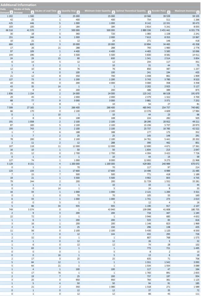
Figure 2 The complete model with real data for ERP ... 47
Figure 3 Additional information that does not interact with ERP but still of interest for strategy decisions. ... 48
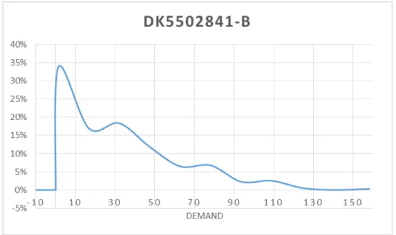
Figure 4 DK5502841-B ... 49
Figure 5 1HSN000003-441 ... 50
Figure 6 Distributed demand over a year of article DK5901318-010 ... 51
Figure 7 Distributed demand over a year of article DK5901351-015 ... 51
Figure 8 How articles in the inventory is distributed by consumption value ... 55
Figure 9 How articles in the inventory is correlated to number of production orders. ... 56
Figure 11 1HSN000003-342 ... 77 Figure 12 DK5101111-002 ... 77 Figure 13 1HSN000003-317 ... 78 Figure 14 DK5101123-016 ... 78 Figure 15 1HSN000102-892 ... 79 Figure 16 1HSN000324-160 ... 79
TABLE LIST
Table 1 Example table of fill rates depending on the variable e ... 18Table 2 There are different equations for q* depending on the interval of e... 18
Table 3 Table of proposed Safety Stock calculation methods. ... 22
Table 4 Example of how different service levels affect the safety factor... 22
Table 5 Safety Stock example values. ... 23
Table 6 Safety Stock results with SERV 1 and SERV2 ... 24
Table 7 How the accumulated expenditure correlates with articles in inventory... 25
Table 8 Classes connected to values of CV ... 25
Table 9 1-2-3 Classification System ... 34
Table 10 Interviewed Companies ... 36
Table 11 Necessary data for calculations to the first theoretical comparison. ... 44
Table 12 Values for optimal order quantity (Q), reorder point (R) and tot total inventory costs (TC)... 45
Table 13 Example of the savings of certain articles. ... 52
DESIGNATIONS
Designation Description Unit
c Item cost Kr, €, $, …
C Annual inventory cost Kr, €, $, … d Mean demand per unit of time Units D Annual average demand Units
F Fill rate %
h Carrying cost Kr, €, $, …
k Expected cost per unit of time Kr, €, $, … Pr Probability of stockout %
Q Optimal order quantity Units QW Optimal order quantity by Wilson Units
R Reorder point Units
s Shortage cost per physical unit Kr, €, $, …
S Ordering cost Kr, €, $, …
Z Expected shortage per cycle %
µ Average demand Units
µ’ Average lead time demand Units
σ'
Standard deviation of lead timedemand Units
σD Standard deviation of demand Units
ABBREVIATIONS
Abbreviation DescriptionEOQ Economic Order Quantity ERP Enterprise Resource Planning MRP Material Requirements Planning OTD On Time Delivery
Q* Optimal quantity ROP Reorder Point SF Safety Factor SL Service Level
1
INTRODUCTION
Logistic management is a major part of a company’s ability to be productive and is of no small concern for the companies in the world. It is one of the first steps, and among the crucial ones of the supply chain and no industry are immune to its challenges. Prajogo, Oke, and Olhager (2016) express that external processes such as logistics have a direct effect on operational performance. A company who, intentionally or unintentionally, neglects its inventory management could deteriorate a company’s performance and consequently reject opportunities for profit (Eroglu & Hofer, 2011). This matter is consequently of interest to all businesses regardless of size (Capkun, Hameri, & Weiss, 2009).
Capkun, Hameri, and Weiss (2009) research indicates that a corporation which has implemented a well-designed inventory routine and procurement processes can reap the rewards with reduced inventory costs, improved lead times, et cetera. An organization who operate effective logistic management increases their customer satisfaction and chance to gain a competitive advantage over those overlooks this focus.
1.1
Background
Large corporations with a high flow of material require a well-designed supply chain for storing material, maintaining productivity, on time deliveries and less production shortage. A well-structured logistic system can make the company more efficient and productive.
Inventories for a company can be expensive, with a significant amount of the current assets as raw material. If the stock balance numbers are not up to date regarding actual inventory levels, it causes multiple conflicts with a loss of production and late deliveries with possible losses of customers and added costs as a result. Poor inventory management has an impact on the company’s working capital, output and customer service. (Rajeev, 2008)
Throughout the 20th and 21st century, there is a substantial amount of research covering the
optimal order quantity, order point, and overall inventory management with the purpose to minimize inventory costs. Ford W. Harris gives one of the first published papers regarding the most optimal order quantity in 1913 (Erlenkotter, 1989). Harris (1990) research showed the importance of understanding the economic size of lots and its value to a company. His formula had the objective to solve a common issue among manufacturer, the most
economical quantity to order. He emphasized that a qualified judgment is a significant factor and difficult to replace with mathematical formulas. Hence no company should unilaterally rely on formulas to determine order quantities. With the knowledge of how much to order, the next step is to decide when to order. An order must be placed at a certain time to fulfill the demands of the production and at the same time not yield overstocks. The early models for optimal order quantity and order point were often combined and followed in a sequence (Patel, 1986).
Available inventory research has not only focused on the purchasing procedure but other areas as well. Rossetti and Achlerkar (2011) discussed whether it is feasible to determine stock levels and parameters for individual articles or if it is more advantageous to determine by grouping instead. The research is limited on this topic, and what is considered large-scale inventory is yet undefined. For instance, Moore and Cox (1992) have conducted research on forecast models for large-scale inventory, but then the stock keeping units have an enormous range from 250-80,000. With a large inventory, it may be difficult for employees to keep track of all articles and a procedure for determining the important items may be in place. A classification of articles has the purpose of analyzing the inventory and offering decisions support on stock control, invested time and ideal service levels for individual articles; it narrows down the available options. (Teunter, Babai, & Syntetos, 2010)
Dion, Hasey, Dorin, and Lundin (1991) shows that absence of specific and standardized routines for the employees can lead to difficulties regarding inventory level. It is a complicated procedure to overview stocks, and poor performance leads to stockout or
overstock instead. Stockouts or poor material flow delays production which in return hinders deliveries to customers, a loss of income due to delay fees and prevents billing. An
interruption in output reduces productivity when the employees are at their working stations and do not produce any value for the company.
1.1.1
Problem Statement
ABB Capacitors are looking to develop the procurement policy, and there has been some internal work done on this topic. Insufficient inventory policies lead to unnecessary administrative costs and strain on company resources as exemplified by Dion et al. (1991) article. These costs can be cut with a policy including a calculation model and inventory analysis that optimize the inventory procedures based on the local prerequisites. This problem is not limited to ABB Capacitors alone nor their interest for a high-performance inventory policy. As Capkun, Hameri, and Weiss (2009) have shown in their research, there is a strong correlation between the inventory performance and the company’s financial results, and it is distributed through manufacturing industries.
With more than 4000 articles is ABB Capacitors considered, according to Moore and Cox (1992), a manufacturer with a large-scale inventory. A question is raised along the expression large-scale, with this range of articles it is bound that some are consistently required in production, and some are less frequent. The procurement policy would not provide any improvements if it only hinders stockouts at the expense of overstocking and vice versa, and if the available data is too deficient for an accurate outcome. Therefore, a method with stochastic demand by Axsäter (2006) and Joon-Seok and Jung (2009) may be more suitable for these types of circumstances rather than Harris (1990) method. These methods share several similarities, and the goal is the same. Find the optimal quantity of items in stock in regards to the production demand and delivery lead time to minimize inventory costs (Moon & Choi, 1994; Wilson, 1991).
instructs employees dealing with material flow consisting of a high variety of different articles. The production demand necessitates an increase of the inventory’s fill rate which is problematic due to the objective to decrease the tied-up capital. One underlying reason for the low fill rate is the lack of a systematic approach to purchasing articles to stock.
ABB Capacitors requires a new policy framework that contains these parameters and setting up the process of order intervals, order quantities, the size of the safety stock and a plan to evaluate whether it is financially beneficial to keep articles in stock. Available research focuses primarily if a company should manufacture-to-order or to stock (Beemsterboer, Land, & Teunter, 2016; Chen, Tai, & Yang, 2014). This research focuses mainly on production optimization and less on the actual purchasing of material. Should manufacturing companies control the inventory levels by forecasts based on the production (order-to-stock) or when an order is placed (order-to-order), and how are these alternatives chosen? The research on this matter is not extensive which provides an opportunity to apply existing research about make-to-stock and make-to-order on a new territory. ABB Capacitors will work as the case study upon which the procurement policy is tested on to verify and validate the result.
1.2
Purpose of the Study
The purpose of this degree project is to design a procurement policy which helps to minimize capital tied up in inventory.
As earlier described in this chapter, the focus of this degree project is to optimize a
procurement policy to minimize the inventory costs. The problem is dealt with a technical and financial perspective. The issue at hand is not solved by considering managerial objectives or its influence within logistic flows. The ambition is to design a new inventory policy that is easy to understand and with little means reduce inventory cost and
subsequently improve a company’s competitiveness. This inventory policy framework could be useful for businesses that are at the very start of the process to implement a systematic framework to the logistical department and desires guidance in their work progress. It could in addition help explaining the similar difficulties dealing with stochastic demands and variable lead times when designing realistic procurement policy to adjust inventory levels.
1.2.1
Study Question
How can the process for article classification and procurement be improved in a new implementable inventory policy with the objective to reduce inventory costs.
1.3
Scope and Limitations
The currently applied purchasing procedures and working routines of the case study will be taken to account when creating the model for applicability but not affect the design itself. The used mathematical formulas and methodologies’ is chosen independently. Possible
limitations of the case study and its effect on the model’s generalizability are elaborated in the conclusion. The conducted model will be suitable for current items in use where data is present.
• The model should be based on critical inventory factors such as expenditure, holding cost, annual and daily demand from production and lead time for deliveries.
• The classification system requires being displayed in a simple and structured manner. • To receive an adequate representation of the complexity of production fluctuations,
the concept model will include variations in demand and lead times.
• Only look at other ABB companies and close connected suppliers with a similar organization.
• Staggered pricing is not considered.
It is estimated that an arbitrary result can be achieved with these general restrictions based on the presented information in the problem statement. Thus, any other restrictions which affect the procurement policy and working procedures are ignored for simplification reasons.
2
INVENTORY CONTROL
This chapter describes acknowledged inventory replenishment methods from early 20th
century in the previous stage of mass-production. Up to recent research with quick response methods in a global competition were time and flexibility is of the essence, along with an overall approach to inventory management.
2.1
Methods to Calculate the Optimal Order Quantity
Several methods are presented for calculating the optimal order quantity in the following section.
2.1.1
Economic Order Quantity
The Economic Order Quantity model was developed in 1913 by Ford W. Harris, and it is one of the oldest methods (Y. Zhu, Wang, Li, & Cai, 2016). The model determines the most optimal order quantity based on the cost of the order and the cost of holding inventory (Zinn & Charnes, 2005). To calculate the order quantity with EOQ one need to know the annual demand quantity, the cost of ordering, item unit cost and holding cost per monetary unit per year (Heizer & Render, 2014; Vasconcelos & Marques, 2000; Y. Zhu et al., 2016). The
formula is often called the Wilson Model (Yang & Fu, 2016). Q𝑊𝑊= �2 × D × Sh × c
Formula 1
The model is based on several assumptions. The demand and lead time are known and relatively constant, orders are delivered in one batch, the model does not consider staggered pricing and is designed to avoid stockouts (Yang & Fu, 2016). The EOQ formula is considered robust. Changes in demand, holding and order cost and quantity makes somewhat small differences in total cost (Heizer & Render, 2014).
Maddah and Noueihed (2017) finds that EOQ, by itself, can confidently be used when the delivery lead time is short, about one day. However, when the lead time increases, stochastic inventory models are preferred.
2.1.2
Continuous Review (R, Q) Model Gamma Distributed
The (R, Q) inventory model is a continuous review model. The goal of the model is to
minimize the cost with respect to order quantity 𝑄𝑄 and reorder point 𝑅𝑅 (Moon & Choi, 1994; Vasconcelos & Marques, 2000). It is possible to do this with an iterative method, but for simplicity and applicability, has it been research regarding finding the optimal values for 𝑄𝑄 and 𝑅𝑅 numerically (Das, 1976; Vasconcelos & Marques, 2000).
The procedure in this degree project is focused on the work by Vasconcelos & Marques (2000), but theories from others as well.
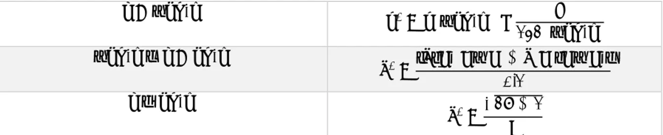
The objective function includes the ordering cost, shortage cost per physical unit, expected shortage per cycle, annual average demand, order quantity, carrying cost, item cost, reorder point and mean demand per unit of time and is described as:
min 𝐶𝐶𝑄𝑄,𝑅𝑅 = (𝑆𝑆 + 𝑠𝑠 × 𝑍𝑍) ×𝐷𝐷𝑄𝑄 + ℎ × 𝑐𝑐 �𝑄𝑄2 + 𝑅𝑅 − 𝑑𝑑�
Formula 2
There is a certain procedure to solve the equation and to find the optimal values for 𝑄𝑄 and 𝑅𝑅. The first step is to calculate EOQ provided by Wilson and described in an earlier chapter (2.1.1 Economic Order Quantity). The second step is to calculate 𝑍𝑍/(𝑑𝑑 × 𝑃𝑃𝑟𝑟) by an
approximation which Vasconcelos & Marques (2000) made from Johnston (1980) which contain the variables expected shortage per cycle, mean demand per unit of time and
probability of stockout. The approximations include constants and the variable 𝑔𝑔 which is the mean demand per unit of time divided by the standard deviation of lead time demand, the quota is raised to the power of two.
𝑔𝑔 = �𝜎𝜎′�𝑑𝑑 2 Formula 3 𝑍𝑍 𝑑𝑑 × 𝑃𝑃𝑟𝑟 = 0.11518267 + 1.0230964 𝑔𝑔 − 0.12294566 𝑔𝑔2 Formula 4
With that number known, the third step is to calculate 𝑄𝑄/𝑑𝑑 by If 𝑔𝑔 ≠ 1 and 0.5 < 𝑔𝑔 < 12. 𝑄𝑄 𝑑𝑑 = 𝑍𝑍 𝑑𝑑 × 𝑃𝑃𝑟𝑟+ �� 𝑍𝑍 𝑑𝑑 × 𝑃𝑃𝑟𝑟� 2 + �𝑄𝑄𝑑𝑑 �𝑊𝑊 2 Formula 5
If 𝑔𝑔 = 1
𝑄𝑄
𝑑𝑑 = 1 +�1 + �𝑄𝑄𝑑𝑑 �𝑊𝑊
2
Formula 6
The first variable 𝑄𝑄 is now determined, and 𝑅𝑅 is the remaining one. 𝑅𝑅 can be calculated in several ways. With a tool like Matlab, 𝑅𝑅 can be computed by solving for 𝑅𝑅 in the formula below because everything else is known.
𝑃𝑃𝑟𝑟 = � 𝑓𝑓(𝑥𝑥)𝑑𝑑𝑥𝑥 ∞
𝑅𝑅
Formula 7
Where 𝑓𝑓(𝑥𝑥) is the gamma density distribution which can be calculated by Formula 8 to Formula 10 provided by (Axsäter, 2015).
𝑓𝑓(𝑥𝑥) =𝜆𝜆(𝜆𝜆𝑥𝑥)𝑔𝑔−1𝑒𝑒−𝜆𝜆𝜆𝜆 Γ(𝑔𝑔) , 𝑥𝑥 ≥ 0 Formula 8 Γ(𝑔𝑔) = � 𝑥𝑥𝑟𝑟−1𝑒𝑒−𝜆𝜆𝑑𝑑𝑥𝑥 ∞ 0 Formula 9 𝜆𝜆 =𝜎𝜎′𝑑𝑑2 Formula 10
Since 𝑅𝑅 is unknown and it is hard for a company to estimate the probability of stockout 𝑃𝑃𝑟𝑟, it
can be set as a fixed value, e.g. five or ten percent (Vasconcelos & Marques, 2000). Instead of calculating the gamma density distribution, a numerical approximation is given below.
𝑍𝑍 𝑑𝑑 × 𝑃𝑃𝑟𝑟 = 𝐴𝐴1+ 𝐴𝐴2𝑃𝑃𝑟𝑟 Formula 11 𝐴𝐴1 = 0.094608205 + 1.0130969 ×𝑔𝑔 − 0.095595537 × �1 1𝑔𝑔� 2 𝐴𝐴2= 0.20574471 + 0.099995001 ×𝑔𝑔 − 0.27350124 × �1 1𝑔𝑔� 2
𝑅𝑅 𝜎𝜎′ = 𝐴𝐴3+ 𝐴𝐴4 × ln(𝑃𝑃𝑟𝑟) + 𝐴𝐴5𝑃𝑃𝑟𝑟2+ 𝐴𝐴6𝑃𝑃𝑟𝑟 × ln(𝑔𝑔) Formula 12 𝐴𝐴3= 0.0106179 − 0.0156841 × 𝑔𝑔2+ 1.66011 × ln(𝑔𝑔) − 0.365992 × (ln(𝑔𝑔))2+ 0.145241 × 𝑔𝑔 × ln(𝑔𝑔) 𝐴𝐴4= −0.998223 − 0.00231704 × 𝑔𝑔2+ 0.357741 × ln(𝑔𝑔) − 0.106577 × (ln(𝑔𝑔))2 + 0.0201662 × 𝑔𝑔 × ln(𝑔𝑔) 𝐴𝐴5= −1.48338 − 0.000741918 × 𝑔𝑔2+1.46426𝑔𝑔 − 0.206282 × ln(𝑔𝑔) 𝐴𝐴6= 2.76031 − 2.72033 × 𝑔𝑔 − 0.0544844 × 𝑔𝑔2+ 3.13504 × ln(𝑔𝑔) + 1.04581 × 𝑔𝑔 × ln(𝑔𝑔)
With the constants calculated, 𝑅𝑅/𝜎𝜎′ can be calculated with Formula 12 and thereafter 𝑅𝑅.
2.1.3
Continuous Review (R, Q) Normally Distributed
Axsäter (2006) presents a numerical method for determining the most optimal order
quantity and reorder point when the lead time demand is normally distributed. The objective function is to minimize the total overall cost with a fill rate constraint.
𝑘𝑘 = ℎ �𝑅𝑅 +𝑄𝑄2 − 𝜇𝜇′� + ℎ ×𝜎𝜎′2 𝑄𝑄 �𝐻𝐻 � 𝑅𝑅 − 𝜇𝜇′ 𝜎𝜎′ � − 𝐻𝐻 � 𝑅𝑅 + 𝑄𝑄 − 𝜇𝜇′ 𝜎𝜎′ � � + 𝑆𝑆𝑑𝑑 𝑄𝑄 Formula 13 𝐹𝐹 = 1 − 𝑇𝑇(0) = 1 −𝜎𝜎𝑄𝑄 �𝐺𝐺 �′ 𝑅𝑅 − 𝜇𝜇𝜎𝜎′ ′� − 𝐺𝐺 �𝑅𝑅 + 𝑄𝑄 − 𝜇𝜇𝜎𝜎′ ′� � Formula 14
To simplify Formula 13 and Formula 14, four parameters are created and substituted into the formulas.
𝑎𝑎 =ℎ𝜎𝜎𝑘𝑘′ Formula 15
𝑞𝑞 =𝜎𝜎𝑄𝑄′ Formula 16
𝑟𝑟 =𝑅𝑅−𝜇𝜇𝜎𝜎′′ Formula 17
𝐸𝐸 =ℎ𝜎𝜎𝑆𝑆𝑆𝑆′2 Formula 18
𝑎𝑎 = 𝑟𝑟 +𝑞𝑞 2 +[𝐻𝐻(𝑟𝑟) − 𝐻𝐻(𝑟𝑟 + 𝑞𝑞)] + 𝐸𝐸 𝑞𝑞 Formula 19 𝐹𝐹 =1𝑞𝑞[𝐺𝐺(𝑟𝑟) − 𝐺𝐺(𝑟𝑟 + 𝑞𝑞)] Formula 20
Axsäter (2006) then provides a step-by-step solution method where the optimal order quantity is determined first and thereafter the reorder point.
The first step is to calculate 𝐸𝐸 and 𝑒𝑒 = ln(𝐸𝐸) to obtain 𝑞𝑞∗. Using the table provided in the
journal or the more detailed table provided on Sven Axsäters profile page (Lund University, 2017). The fill rate is chosen, and 𝑒𝑒 is calculated to obtain 𝑞𝑞∗ from the table. Interpolating in
the full table is possible.
Below is a smaller version of the table as an example. The table can be created by solving Formula 19 and Formula 20 for every value of E and fill rate (Axsäter, 2006). This example table should not be used for the calculations.
Table 1 Example table of fill rates depending on the variable e.
e S 60% 70% 80% 90% 95% 99% -15.0 0.0190 0.0173 0.0157 0.0140 0.0130 0.0116 0.0 2.9462 2.6421 2.3964 2.1675 2.0373 1.8756 1.0 4.3138 3.8249 3.4659 3.1593 2.9967 2.8070 1.5 5.3105 4.6685 4.2223 3.8634 3.6817 3.4772 2.0 6.6362 5.7740 5.1995 4.7680 4.5614 4.3384 15.0 4261.60 3651.80 3196.20 2841.06 2691.54 2582.79
As can be seen in the smaller version of the table, values of 𝑞𝑞∗ is only available for values of 𝑒𝑒
in the interval −15.0 ≤ 𝑒𝑒 < 15.0. When the values are outside of the table, 𝑞𝑞∗ is determined
by another method. In case two where the values are within the given range, 𝑒𝑒 is the largest table value that is closest to the actual 𝑒𝑒 and 𝑒𝑒 is the lower table value that is the closest to the actual 𝑒𝑒.
Table 2 There are different equations for q* depending on the interval of e.
𝒆𝒆 < −𝟏𝟏𝟏𝟏. 𝟎𝟎 𝒒𝒒∗= 𝒒𝒒(−𝟏𝟏𝟏𝟏. 𝟎𝟎) × 𝑬𝑬 𝐞𝐞𝐞𝐞𝐞𝐞(−𝟏𝟏𝟏𝟏. 𝟎𝟎) −𝟏𝟏𝟏𝟏. 𝟎𝟎 ≤ 𝒆𝒆 < 𝟏𝟏𝟏𝟏. 𝟎𝟎 𝑞𝑞∗=�𝑞𝑞�𝑒𝑒�(𝑒𝑒 − 𝑒𝑒) + 𝑞𝑞(𝑒𝑒)�𝑒𝑒 − 𝑒𝑒�� 0.1 𝒆𝒆 ≥ 𝟏𝟏𝟏𝟏. 𝟎𝟎 𝑞𝑞∗=√2𝐸𝐸 + 1 𝑆𝑆
The value of 𝑞𝑞∗ is obtained, the next step is to calculate the value of 𝑟𝑟∗. To do that Formula
20 is used since every value is known except for 𝑟𝑟. As can be seen 𝑟𝑟 is the function variable of 𝐺𝐺. The variables 𝑟𝑟∗ and 𝑞𝑞∗ replaces 𝑟𝑟 and 𝑞𝑞 in the formulas.
𝐺𝐺(𝑟𝑟) = � (𝑣𝑣 − 𝑟𝑟)𝜑𝜑(𝑣𝑣)𝑑𝑑𝑣𝑣 = 𝜑𝜑(𝑟𝑟) − 𝑟𝑟�1 − 𝜙𝜙(𝑟𝑟)�∞
𝑟𝑟
Formula 21
Where 𝜑𝜑(𝑟𝑟) and 𝜙𝜙(𝑟𝑟) can be obtained from Formula 22 and Formula 23 (Axsäter, 2015). 𝜑𝜑(𝑟𝑟) is the density function and, 𝜙𝜙(𝑟𝑟) is the distribution function.
𝜑𝜑(𝑟𝑟) = 1 √2𝜋𝜋exp �− 𝑟𝑟2 2 � , −∞ < 𝑟𝑟 < ∞ Formula 22 𝜙𝜙(𝑟𝑟) = � 1 √2𝜋𝜋exp �− 𝑢𝑢2 2 � 𝑑𝑑𝑢𝑢 𝑟𝑟 −∞ Formula 23
It is possible to not do the integration and obtain 𝜙𝜙(𝑟𝑟). A simpler way is to use the Excel formula 𝑁𝑁𝑁𝑁𝑅𝑅𝑁𝑁. 𝑆𝑆. 𝐷𝐷𝐷𝐷𝑆𝑆𝑇𝑇(𝑟𝑟; 𝑇𝑇𝑅𝑅𝑇𝑇𝐸𝐸). With a calculation software, solve for 𝑟𝑟 to get the
appropriate fill rate. Repeat the procedure to find 𝐺𝐺(𝑟𝑟 + 𝑞𝑞) then the optimal 𝑄𝑄 and 𝑅𝑅 can be calculated with Formula 24 and Formula 25.
𝑄𝑄 = 𝑞𝑞∗𝜎𝜎′
Formula 24
𝑅𝑅 = 𝑟𝑟∗𝜎𝜎′+ 𝜇𝜇′
Formula 25
2.1.4
Other Available Models
There are plentiful types of models for calculating the optimal order quantity, two common methods are Quick Response and (s, S) policy which receive a brief explanation.
2.1.4.1.
Quick Response
The Quick Response (QR) is one of the most known methods to use in inventory
management. The QR method determines an order quantity that is needed until the next delivery, nothing more. The formula for order quantity then becomes:
𝑄𝑄𝑅𝑅 𝑁𝑁𝑟𝑟𝑑𝑑𝑒𝑒𝑟𝑟 𝑄𝑄𝑢𝑢𝑎𝑎𝑄𝑄𝑄𝑄𝑄𝑄𝑄𝑄𝑄𝑄 = 𝐷𝐷𝑎𝑎𝑄𝑄𝐷𝐷𝑄𝑄 𝐷𝐷𝑒𝑒𝐷𝐷𝑎𝑎𝑄𝑄𝑑𝑑 × 𝑇𝑇𝑄𝑄𝐷𝐷𝑒𝑒 𝑇𝑇𝑄𝑄𝑄𝑄𝑄𝑄𝐷𝐷 𝑁𝑁𝑒𝑒𝑥𝑥𝑄𝑄 𝐷𝐷𝑒𝑒𝐷𝐷𝑄𝑄𝑣𝑣𝑒𝑒𝑟𝑟𝑄𝑄
Formula 26
As can be noted, it is a simple method that does not consider other relevant variables as mentioned in previous sections. Zinn & Charnes (2005) says that more businesses are going
possible, which the QR method is good at. There is also a risk that companies have an extensive inventory of products that is never going to be used and the holding cost of that. The QR method is most often used when the time between deliveries is short. Because of that, the company needs to be cautious with which items they use it for. If the ordering cost is high, it might be better to use an alternative method, since the benefits of QR may be neglected. If the demand is high for an item or the unit is of high value, there is more advantage in using QR. (Zinn & Charnes, 2005)
2.1.4.2.
(s, S) Policy
The continuous review (s, S)-policy is a similar policy to the continuous review (R, Q) policy. When the inventory level drops below a level 𝑠𝑠, an order quantity 𝑆𝑆 is ordered. The order quantity 𝑆𝑆 is the maximum level. In comparison to the (R, Q)-policy, 𝑠𝑠 is the same as 𝑅𝑅, and 𝑄𝑄 is equivalent to 𝑆𝑆 − 𝑠𝑠. (Axsäter, 2015)
2.2
Determining the Reorder Point
There are two main questions when discussing ordering, how much to order and when to order. Reorder point (ROP) is about the latter when to order. An order is placed when the level of inventory reaches a specific level, and together this is often called a QR Policy (Kurbel, 2013). When the production is constant with minimal disturbances, the reorder point it is relatively easy to set a fixed, optimal and continuous ordering point. Difficulties arise when demand is uncertain and lead time is unfixed (Tamura, Morizawa, & Nagasawa, 2010). The more basic models assume that companies let the inventory level reach zero before ordering and that orders are received at the same time as the order is placed (Heizer & Render, 2014).
The mathematic formula for ROP is:
𝑅𝑅𝑁𝑁𝑃𝑃 = 𝐷𝐷𝑒𝑒𝐷𝐷𝑎𝑎𝑄𝑄𝑑𝑑 𝑝𝑝𝑒𝑒𝑟𝑟 𝑑𝑑𝑎𝑎𝑄𝑄 × 𝐿𝐿𝑒𝑒𝑎𝑎𝑑𝑑 𝑄𝑄𝑄𝑄𝐷𝐷𝑒𝑒 𝑓𝑓𝑓𝑓𝑟𝑟 𝑎𝑎 𝑓𝑓𝑟𝑟𝑑𝑑𝑒𝑒𝑟𝑟 𝑄𝑄𝑄𝑄 𝑑𝑑𝑎𝑎𝑄𝑄𝑠𝑠
Formula 27
The demand per day is a set value and does not vary over time and the lead time for an order is a set value. Heizer and Render (2014) mentions that when the values are not set, a slight change to the formula is to add safety stock as well. The formula then changes to:
𝑅𝑅𝑁𝑁𝑃𝑃 = 𝐷𝐷𝑒𝑒𝐷𝐷𝑎𝑎𝑄𝑄𝑑𝑑 𝑝𝑝𝑒𝑒𝑟𝑟 𝑑𝑑𝑎𝑎𝑄𝑄 × 𝐿𝐿𝑒𝑒𝑎𝑎𝑑𝑑 𝑄𝑄𝑄𝑄𝐷𝐷𝑒𝑒 𝑓𝑓𝑓𝑓𝑟𝑟 𝑎𝑎 𝑓𝑓𝑟𝑟𝑑𝑑𝑒𝑒𝑟𝑟 𝑄𝑄𝑄𝑄 𝑑𝑑𝑎𝑎𝑄𝑄𝑠𝑠 + 𝑆𝑆𝑎𝑎𝑓𝑓𝑒𝑒𝑄𝑄𝑄𝑄 𝑆𝑆𝑄𝑄𝑓𝑓𝑐𝑐𝑘𝑘
2.3
Safety Stock
The definition of safety stock (ss) according to Heizer and Render (2014) is:
“Extra stock to allow for uneven demand; a buffer.” (p. 524).
The need for safety stock arises when there are variabilities in customer demand, lead times, production and any other source that can affect the product itself. The ambition of the company should be to minimize the safety stock as much as possible since inventories can be costly for the company. (Heizer & Render, 2014)
Many companies want to adapt to smaller lot sizes because it allows the company to be more flexible, defects will be easier to spot, easier handling of material and reduction in lead time. The risks are that the company is more vulnerable for stockouts, hence the need for a safety stock (Natarajan & Goyal, 1994).
The commonly used MRP strategy exposes companies for stockouts since the aim for it is to minimize or completely avoid safety stocks at every stage in the manufacturing. The dilemma is that a high service level ultimately requires some safety stock (Dellaert & Jeunet, 2005). The challenges with upholding a high service level and the necessary safety stock are where to store these items and what the most optimal quantity is (De Bodt, Van Wassenhove, &
Gelders, 1982).
The formula for calculating the quantity of the safety stock level is: 𝑆𝑆𝑆𝑆 = 𝑆𝑆𝐹𝐹(𝑆𝑆𝐿𝐿) × 𝜎𝜎𝐷𝐷
Formula 29
The formula is often considered as the standard method for calculating the safety stock level, where SL is the service level which can be determined from a table of standard scores and 𝜎𝜎𝐷𝐷
is the standard deviation of demand (Schmidt, Hartmann, & Nyhuis, 2012). The same formula is described by both Schmidt et al. (2012) and Heizer and Render (2014), and it is assumed that the demand is normally distributed. The calculation is often extended to consider other variables as lead time, lot size, reorder point, the risk of stockouts, forecasts (Heizer & Render, 2014; Natarajan & Goyal, 1994; Schmidt et al., 2012).
2.3.1
Uncertainties with Safety Stock
Schmidt et al. (2012) made a comparison of several different methods for calculating the most optimal safety stock level. They found that none of the tested methods were superior but rather dependable on the circumstances. If the variance of replenishment time is low and the variance of demand could be either low, medium or high, the standard formula, Formula 29, could be used. If the variance of replenishment time is medium or high and variance of demand is high, Formula 30 provided below is a suitable method. (Schmidt et al., 2012)
𝑆𝑆𝑆𝑆 = 𝑆𝑆𝐹𝐹(𝑆𝑆𝐿𝐿) × �(𝐴𝐴𝑣𝑣𝑒𝑒𝑟𝑟𝑎𝑎𝑔𝑔𝑒𝑒 𝐷𝐷𝑒𝑒𝑎𝑎𝑑𝑑 𝑄𝑄𝑄𝑄𝐷𝐷𝑒𝑒 × 𝜎𝜎𝐷𝐷2) + (𝐴𝐴𝑣𝑣𝑒𝑒𝑟𝑟𝑎𝑎𝑔𝑔𝑒𝑒 𝑑𝑑𝑎𝑎𝑄𝑄𝐷𝐷𝑄𝑄 𝑑𝑑𝑒𝑒𝐷𝐷𝑎𝑎𝑄𝑄𝑑𝑑)2𝜎𝜎𝐿𝐿𝐿𝐿2 Formula 30
When there are deviations in lead time but not in demand, Formula 30 becomes: 𝑆𝑆𝑆𝑆 = 𝑆𝑆𝐹𝐹(𝑆𝑆𝐿𝐿) × 𝐴𝐴𝑣𝑣𝑒𝑒𝑟𝑟𝑎𝑎𝑔𝑔𝑒𝑒 𝑑𝑑𝑎𝑎𝑄𝑄𝐷𝐷𝑄𝑄 𝑑𝑑𝑒𝑒𝐷𝐷𝑎𝑎𝑄𝑄𝑑𝑑 × 𝜎𝜎𝐿𝐿𝐿𝐿
Formula 31
When there are deviations in demand but not in lead time, Formula 30 becomes: 𝑆𝑆𝑆𝑆 = 𝑆𝑆𝐹𝐹(𝑆𝑆𝐿𝐿) × 𝜎𝜎𝐷𝐷 × �𝐴𝐴𝑣𝑣𝑒𝑒𝑟𝑟𝑎𝑎𝑔𝑔𝑒𝑒 𝐷𝐷𝑒𝑒𝑎𝑎𝑑𝑑 𝑄𝑄𝑄𝑄𝐷𝐷𝑒𝑒
Formula 32
Presented below is a table of suggested method based on a level of variance in replenishment time and level of variance in demand.
Table 3 Table of proposed Safety Stock calculation methods. (own)
Variance of replenishment time /
Variance of demand No variance Variance
Variance Formula 31 Formula 30
No variance Expected usage during lead time Formula 32
2.3.2
Service Levels
There are two widely known methods for calculating the service level for the inventory (Axsäter, 2015). SERV1 which is the probability of no stockout per order cycle and SERV2 is the amount of demand that can be satisfied immediately from stock (Axsäter, 2015). The service level methods are used for decreasing or increasing the safety stock level by a certain factor. It can be seen in the example table, Table 6, what the effect is of the both service levels and if none at all would be used. There are different advantages and disadvantages with both methods. An advantage is that SERV1 can easily be calculated in Excel with the formula 𝑁𝑁𝑁𝑁𝑅𝑅𝑁𝑁. 𝑆𝑆. 𝐷𝐷𝑁𝑁𝐼𝐼(𝑃𝑃𝑟𝑟𝑓𝑓𝑃𝑃𝑎𝑎𝑃𝑃𝑄𝑄𝐷𝐷𝑄𝑄𝑄𝑄𝑄𝑄) which is the inverse of the cumulative standard normal distribution with mean zero and standard deviation of one (Microsoft, 2017).
Table 4 Example of how different service levels affect the safety factor.
Service Level 80% 85% 90% 95% 97% 98% 99%
Safety Factor 0.842 1.036 1.282 1.645 1.881 2.054 2.326
A disadvantage with SERV1 is that it has nothing to do with the order quantity. If the demand per year is 1000 units and the optimal order quantity is calculated to 900. It is not necessary then to have an oversized safety stock. If the order quantity is determined small compared to the total demand, SERV1 can be insufficient. (Axsäter, 2015).
Before one can calculate SERV2, 𝑆𝑆𝐿𝐿(𝑘𝑘) needs to be computed, thereafter a safety factor can be found in a table or calculated (Mattsson, 2010b).
𝑆𝑆𝐿𝐿(𝑘𝑘) =�1 − 𝑆𝑆𝐿𝐿100� × 𝑄𝑄𝜎𝜎′
Formula 33
The result of Formula 33 can then be found in a table (Mattsson, 2010a) with the
corresponding safety factor. The safety factor, 𝑘𝑘, can also be calculated with several steps: 𝑧𝑧 = �ln � 25 �𝑆𝑆𝐿𝐿(𝑘𝑘)�2� Formula 34 𝑘𝑘 = 𝑎𝑎0+ 𝑎𝑎1 × 𝑧𝑧 + 𝑎𝑎2× 𝑧𝑧2+ 𝑎𝑎3 × 𝑧𝑧3 𝑃𝑃0+ 𝑃𝑃1 × 𝑧𝑧 + 𝑃𝑃2 × 𝑧𝑧2+ 𝑃𝑃3 × 𝑧𝑧3+ 𝑃𝑃4 × 𝑧𝑧4 Formula 35
Where the constants 𝑎𝑎0−3 and 𝑃𝑃0−4 are:
𝑎𝑎0= −5.3925569 𝑃𝑃0= 1 𝑎𝑎1= 5.6211054 𝑃𝑃1= −0.72496485 𝑎𝑎2= −3.8836830 𝑃𝑃2= 0.507326622 𝑎𝑎3= 1.0897299 𝑃𝑃3= 0.0669136868 𝑃𝑃4= 0.00329129114
2.3.3
Numerical Example
To showcase the different results SERV1 and SERV2 gives, a numerical based on article 1HSN000003-317, the example is presented below.
Table 5 Safety Stock example values.
Variable Value
Average lead time 30 days
Standard deviation of lead time 1.60 days
Average daily demand 1835.58 units
Standard deviation of demand 1153.87 units
Order quantity 125 142 units
Standard deviation of lead time demand 6967.23 units
Annual demand 669 987 units
From Table 4, different levels of safety stock are calculated depending on the requested service level with SERV1.
Table 6 Safety Stock results with SERV 1, SERV2 and no safety factor. (own) SERV1 Service Level 80% 85% 90% 95% 97% 98% 99% Safety Stock 5864 7221 8929 11460 13104 14309 16208 SERV2 Service Level 80% 85% 90% 95% 97% 98% 99% Safety Stock -26011 -20397 -14295 -6487 -2184 717 4957 No Safety Factor 6967
2.4
Kanban System
Kanban system is a part of the Lean Production Concept, that manage the supply of material to an assembly line and it has close a relationship to Just-In-Time (Lolli, Gamberini, Giberti, Rimini, & Bondi, 2016). The key principle of Kanban can be defined as a material flow control system with a focus on regulating the quantity of material and time of the production,
preferable as nimble as possible, necessary of the product. It is commonly used with cards as a signal to manage the replenishment of the inventory regarding quantity during time periods and start of production (Lage Junior & Godinho Filho, 2010).
Hence Kanban utilizes the pull system. When a depletion of certain material is detected in the manufacture, the operators uses a card to signal the purchasers and logistical workers to replenish the inventory. It means that the production dictates the frequency and level of replenishment and do so after a real demand and not a forecast. (Ebrahimpour & Modarress Fathi, 1985). Level and choice of implementation vary depending on the situation and desired goals of the users. It exists two major systems, and these are called production Kanban and withdraw Kanban. (Hemamalini & Rajendran, 2000)
During the literature research, a pattern was evidently discovered quite early, and that is that the previously research mainly focus on optimizing Kanban inventory for a single-product supply chain and the production system. It is confirmed by Widyadana, Wee and Chang (2010).
An important part of the Kanban approach is the elements of utilizing a simple and visual system that is easy to understand for affected employees. The inventory is dynamic and self-regulatory with the usage of signals and that it is controlled by real detected demands from the production. Since the overall work process is simple to understand and follow, potential mishaps and risks that someone fails to alert the buyers are relatively low compared to a statistical method based on a forecast.
2.5
Inventory Classification Models
An ABC-analysis is an inventory classification system which utilizes the Pareto principle. The fundamental idea of the analysis, thus Pareto principle, is that there are a few critical
products that associates too much of the expenses. The remaining substantial quantity of the inventory is less expensive, both per article and as a total amount. (Ng, 2007). Ng (2007) describes that the Pareto principles derives from an Italian professor who discovered that 80 percent of the cities wealth was owned by 20 percent of the population, hence the suitable phrase.
“critical few and trivial many.” (Heizer & Render, 2014. p 513).
One of the main purposes to why a manufacturer wants to applicate the ABC analysis is to optimize its managing of the inventories to increase profitability. Besides optimization of the material flow itself, it is also an issue regarding the best way of distributing limited
administrative resources correlating to inventory management since it is inefficient to monitor inexpensive articles at the same level as expensive ones. (Rezaei & Salimi, 2013). The traditional classes are ABC, where A represents articles with the highest expenditure and importance for the company. Follow alphabetical order and C is at the bottom of the scale.
Table 7 How the accumulated expenditure correlates with articles in inventory. (own)
Class Expenditure (%)
Quantity (%)
A
60-80 10-20B
25-35 30C
5-15 50-60The XYZ-analysis categorize the articles of the inventory from another point of view. It
distinguishes the items from each other via the variations in their consumption. For this case, the variations in demand for the production. It is calculated with two variables, the standard deviation of demand and its mean value (Geraghty & Heavey, 2010).
𝑐𝑐𝑣𝑣 =𝜎𝜎µ𝐷𝐷
Formula 36
The analysis is properly used when the operator considers a period and the material consumption within that specific frame. The analysis renders a number which is the
coefficient of variation and represents the range of the consumption levels of that particular item. (Scholz-Reiter, Heger, Meinecke, & Bergmann, 2012)
Table 8 Classes connected to values of CV.(own)
Class Coefficient of variation (C
V)
With these two factors, it is possible to analyze the inventory and receive a proper
understanding with little effort. Some things are still left in the blue though, a screw has a low individual value and probably a small 𝐶𝐶𝑉𝑉 too. It is then easy to have a false sense of security
and step into the trap that an article classified as C, Z is not important for the production. It could be worth the additional effort for a company analyze the number of transactions, stockouts, revenue per article and so forth.
2.6
Make-to-Stock and Make-to-Order
Make-to-stock is one of two ways a company can choose to run its production. Make-to-stock is a strategy when there is a forecast of demand. The quality of the forecast makes the
strategy more or less useful (Kaminsky & Kaya, 2009). Make-to-stock is used when the customer is unknown, and the forecasted demand that aims the production is often called anonymous demand (Kurbel, 2013). Make-to-order is the second strategy in manufacturing. The difference from make-to-stock is that make-to-order have a known buyer and the product can often be customized to the buyers’ requirements (Kurbel, 2013).
The aim for a make-to-order production is to have a high customer satisfaction. That increases the chance for a good reputation and recurring customers. The inventory policy regarding make-to-order is harder to define since the orders are more specified and there is no sufficient method to predict the demand of the articles used in the manufacturing since the orders can be very diverse. These difficulties cause problems with safety stock levels, lead time, higher inventory and holding costs. The sales team also have a challenge regarding what they can promise the customer regarding delivery date and price. (Kurbel, 2013) Make-to-stock items are manufactured with a forecasted demand, and make-to-order production does not begin until an order is received. Shorter delivery lead times should be the focus point to gain an advantage over competitors in to-order system. In a make-to-stock system, accurate predictions of demand and ability to satisfy customer demand for finished goods is the competitive priority. (Shao & Dong, 2012)
Shao and Dong (2012) shows that a strategy for a company should be to manufacture products that have high component cost and little value added in the final assembly in a make-to-stock system. If the individual component holding cost is low compared to the end product and high value is added in the final assembly, a make-to-order system is preferable. Make-to-stock was previously the most common strategy in manufacturing, but nowadays many companies have moved to a make-to-order system (Kaminsky & Kaya, 2009).
Implementing only one of the strategies is unlikely to meet all customers’ demands which are why more manufacturers are utilizing a hybrid system with both strategies (Chen et al., 2014).
2.7
Business IT System
Enterprise Resource Planning (ERP) is an IT system that allows companies to manage the entire spectrum of business operations, from manufacturing focuses such as logistic
planning, production, and distribution of goods to communication and customer service (Yen & Sheu, 2004). Companies face numerous challenges in the global competition and need to respond rapidly to sustain its flexibility, development, and competitiveness throughout the supply chain. ERP is a useful tool to streamline the organization and work like a well-oiled machinery (Tsai, Hwang, Chang, Lai, & Yang, 2011; Yen & Sheu, 2004).
The goal of any implementation is that the new changes generates increased operational profits. The groundwork to realize this objective is to apply certain modifications in the business process to improve critical steps as lead time, productivity, communications, logistical flow, et cetera. (Magnusson & Olsson, 2008)
There are however several drawbacks that each operation manager or corporate leader must consider before a final decision. These systems are often complex, which leads the company down a path with large installment fees, maintenance costs, high expenditure on
administration and employees. Companies are financially exposed with increasing threats from daily production, competitors, and expensive projects during these times. (Magnusson & Olsson, 2008)
Even if these costs might be manageable for companies, other circumstances need to be considered. For instance, how large is the advantage with ERP if a competitor also uses a similar system? Would that not reduce the potential advantage? Perhaps it is more of necessity rather than a potential mean to gain an advantage? The ERP system is used in this degree project to obtain relevant data, i.e. variables needed by the calculations. All variables presented in the formulas is possible to extract hence there is no need to create own data to test or simulate with.
2.8
Suitable Theory for Testing
EOQ, Formula 1, and ROP, Formula 27, are two well-known and used formulas to minimize inventory costs, it is logical to test those in this environment. A model consisting of those is relatively simple and does not provide immense challenges to program them together in one model. A potential weakness is its assumptions, and it is not adequate to determine order-to-stock or order-to-order.
A continuous review provides other opportunities to calculate same variables (2.1.2 Continuous Review (R, Q) Model). It has the same fulfillments as the first model but with additional safety measures by using gamma distribution. This one will always have a higher order quantity. Another interesting aspect which is desired to explore is the interval of 𝑔𝑔. Could that interval be used to help determine order-to-stock or order-to-order?
all. This one is interesting because it is recently developed, from a recognized scientist, and might work as an intermediate between the other two. Whether it can enlighten order-to-stock or order-to-order is at this stage unclear.
Each model should include a calculation for the safety stock, most likely the same since the data will contain both standard deviations and mean numbers. It will not be hard to come by with necessary data for Formula 30.
• Model 1, consisting of 2.1.1 Economic Order Quantity and 2.2 Determining the Reorder Point • Model 2, 2.1.2 Continuous Review (R, Q) Model
• Model 3, 2.1.3 Continuous Review (R, Q) Normally Distributed • Same formulas for calculation of safety stock, 2.3 Safety Stock
3
METHODOLOGY
The following chapter describes the academic approach and methods used in this degree project. The method helps to answer the hypothesis that the model will lower the inventory cost and increase the overall service level.
3.1
Approach
There are several different approaches to reasoning throughout research, deductive,
inductive, and abductive. The deductive approach is a method were the researcher starts out with a hypothesis and testing it empirically with the help of relevant theory. The theory is a big part of deductive approach and contributes to develop the hypothesis, regarding variables and how to evaluate the results. The usefulness is that previous research can be utilized by the researcher. (Blomkvist & Hallin, 2015; Hyde, 2000)
An inductive research approach starts out with observing the problem and finding a theory that explains the results. The empirical material affects the research and used theory (Blomkvist & Hallin, 2015). The third approach, abductive, which is a combination of
deductive and inductive. It is a back and forth kind of approach where the researchers let the empirical material affect the theory and vice versa (Blomkvist & Hallin, 2015).
In this study, it was known that it existed a large proportion of relevant theory to the problem statement and developed hypotheses. The theory outlines the recommended variables that are required for minimizing the overall cost of the inventory. The interviews are not supposed to influence the variables but to highlight certain occurrences surrounding the procurement process. The findings are supposed to complementary conditions to the procurement policy and be a recommendation for further improvement by the company where the case study is carried out. The work process consisted mostly of applying already existing theory on a given problem and conducting interviews. The research approach was deductive since, as mention before, the interviews are not supposed to change the alignment of the work thus the theory is the fundament of this degree project. Instead, the idea with interviews was to have an outside factor which could confirm and strengthen decisions that have been executed as the degree project progressed.
The deductive work process made by Ali and Birley (1999) were chosen, and they outline the basic stages in a deductive research approach which inspired the work process.
• Develop a theoretical framework
• Variables identified for relevant constructs • Instrument development
• Respondents give answers to specific questions
• Answers analyzed in regarding prior theoretical framework
Figure 1 Work procedure of the Degree Project. (own)
Another reason for choosing a deductive approach and why it was suitable is the vast amount of available theory that aims to answer to the hypothesis. Given the theory, relevant variables were identified for data gathering. When the variables were identified, an appropriate model could be designed, and empiric data could be obtained. The data could after that be
compared to the theory to find out what the study object seemed to be missing and input to the variables could be considered. Finally, the outcome from the model could be tested to see if it were working as intended.
3.2
Qualitative and Quantitative Data
Ali and Birley (1999) is describing qualitative research as research that is heavily based on the participant’s point of view and opinions, and it should act as guidance for the research. Hyde (2000) says that qualitative data is based on text rather than numbers. Qualitative methods include observations or interviews (Blomkvist & Hallin, 2015). The interviews in this work are considered qualitative because the respondents’ opinions affected the work to increase the applicability to the organization, and valuable knowledge was given.
The most common description of quantitative research is that it regards data as numbers. Examples of quantitative methods are surveys and statistical methods. The theory about the proposed model indicates that it are numbers intensive with the need of yearly based
statistics (Das, 1976). The study’s scope is moreover to classify the articles based on ABC and XYZ which is a quantitative calculation. The study is foremost a quantitative research with qualitative influences.
3.2.1
Gathering of Data
Two types of data have been collected in this study, primary and secondary data. Primary data are the data that is collected by the researchers for the specific problem with methods that fits the best. Secondary data is the data that has been collected by someone else than the researchers; it already exists, e.g. statistics. (Hox & Boeije, 2005). The primary data in this research consists of interviews while the secondary data consists of statistics and other data from the business software at the organization of the study and information by academic journals and books.
The bulk of the gathered information is made of quantitative data which was gathered with the help of the logistics developer from ERP and QlikView. The collected data includes article name, article number, annual and daily demand, lead time from the supplier, and item cost for all available articles. The data has then been used to calculate new levels of safety stock, order quantity and reorder point. Without that necessary data, the statistical formulas and the models would not function properly or produce a useful result. The secondary data have singlehandedly the highest significance for this research.
3.3
Development of the Procurement Policy
This section describes the development of designing the three models, the inventory analysis and the choice of an implemented concept model, which forms the procurement policy. The development of the calculation model can be described as a two-stage. Firstly, three models are developed which consider both shared and separate variables for the calculations. The results are then compared and evaluated based on their contributed affect to an overlapping procurement policy. The evaluation relies on the approach of the research and general applicability.
The best overall performing model was selected for the second stage to become the purchasing model and the basis of the procurement policy. The second stage exposes the model to multiple theoretical and empirical tests. The theoretical test is a comparison of current parameters, and the empirical test is to see how the production and inventory of the case study perform under these new parameters.
Concept models
• Model 1, consisting of 2.1.1 Economic Order Quantity and 2.2 Determining the Reorder Point • Model 2, 2.1.2 Continuous Review (R, Q) Model
• Model 3, 2.1.3 Continuous Review (R, Q) Normally Distributed • Same formulas for calculation of safety stock, 2.3 Safety Stock
The first constructed model was model 1. It has a primitive but robust design which provides reasonable values for the optimal order quantity and reorder point. The necessary
Business IT System). The model is reliable since the degree of variation of the inputs has a smaller effect on the output.
Discrete variables, constant values, and simplified assumptions indicate that model 1 is suitable for a general implementation for procurement, regardless of business sector. As one of the first mathematical formulas in this area of expertise and developed in a time when limited computing power existed, one must raise a small warning whether the scientific area of research on this matter has progressed or if it is still relevant today. Although Wilson’s formula impact in the latest century is unquestionable (H. Zhu, Liu, & Chen, 2015).
Model 1 could potentially have a noteworthy flaw because one assumption of the calculations is constant production demand. It is not an ideal representation of realistic conditions, and though it might be adequate for a general implementation, it is desired that the concept model can produce a good result in a company’s daily operations by the established parameters. A visual investigation of the articles in the ERP database showed that almost every single one had variations in lead times, demand or both.
There were two underlying reasons if an item had a variation of zero, for lead times or demand. The first one is that there were few deliveries or production orders. Thus, the result is correctly calculated, but the sample size is questionable and might not be statistically reliable. The second case is when the relevant data is missing, for simplification the
variations are set to zero but with the operator’s knowledge that the final calculated values are not completely accurate. This problem is shared with the other two models, but since they include more variables, they should still produce a better overall accuracy. Another issue with model 1, which is known beforehand, is that it does not answer the question or helps to decide when an article should be order-to-stock or order-to-order.
The other two models include a stochastic demand, preferably by more complex calculations to subsequently avoid constant variables. By including complicated calculations via integrals and numerical approximations, the result could improve but to a more demanding
computation. The literature review showed that these calculations were more exhausting and time-consuming than by hand, but their purpose is to be solved by using the calculation of computers. Since computers are more common now than when most previous works were performed, this would not be a hinder for using the models.
With the basic models developed the first staged was completed. It was possible to test and compare these three models via theoretical calculations and proceed with the final
evaluation. The results of optimal order quantity, reorder points and its ability to determine order-to-order or order-to-stock was the main features’ and of highest importance for the decision. Practicality and applicability at the case company were also discussed but not allowed to act as the keystone in this verdict.
3.3.1
Tools
When the models were narrowed down to three the next step were to choose which software was the most suitable for the calculations. The approach of this issue is the degree of
applicability. Multiple software could solve these equations, and the issue is which one was going to be used. For instance, if the number of code lines in Matlab is quite small, compared to Excel, then it would be a huge time-saver. If Matlab would have been used it would require some formatting through Excel anyway. The database is obtained through the QlikView tool and extracted to an Excel file which sometimes requires preparation depending on the data the operator desires, regardless of end-user program. It is not decisive though. Another aspect weighs heavier, hence more crucial is the knowledge among the potential users, whose computer knowledge is limited to ERP and Excel. Out of all employees at the procurement department, only one had knowledge of Matlab, and as will be confirmed by the empirical results, usage of Matlab is extremely limited compared to Excel in these issues. To achieve a higher level of general applicability, it deemed best to conduct a model with Excel instead of Matlab.
Because ERP is the IT-system which all prognoses and historical data are retrieved from, there is no need to create own data to simulate with. In addition to the available database, this multiple-tool is of considerable interest for its capabilities to simulate and conduct experiments in a realistic staging environment. It provides an opportunity to test the concept model with live-data and compare its accuracy to historical results, therefore, validate and verify the model empirically rather than conducting complex mathematical proof.
The conceptual model will be designed independently from the programming capabilities that ERP possess and will not be able to interact either. The settings in ERP will be manually calibrated after the correct variables and values have been computed via the concept model.
3.3.2
Inventory Analysis
At the early stage of investigating and learning ERP, it was discovered that the IT-department conducts ABC-analysis for each ABB business unit upon request. It was decided after a
discussion with a logistical developer at the case study, that the first stage of the ABC analysis should be conducted by themselves because of applicability and comparability.
If an own analysis had been conducted with own theoretical intervals that differ from the IT-departments own, it would not be possible to compare articles over time with previous analyses, and it would be a waste of time to conduct something someone else already knew. The article analysis could, therefore, be extended by investigating other relevant variables, for instance, the number of transactions.
The number of transactions variable (123) is significant and should not be neglected, articles which have a low value can still carry high administrative costs because of a vast number of transactions. Hence, they are possibly critical for the production process, but with their low value, this is not shown. With this extend ABC-XYZ and transaction analysis there is a base