ANALYSIS OF THE REPEATABILITY OF TIME-LAPSE 3D VSP MULTICOMPONENT SURVEYS, DELHI
FIELD
by
c
Copyright by Mariana Fernandes de Carvalho, 2013 All Rights Reserved
A thesis submitted to the Faculty and the Board of Trustees of the Colorado School of Mines in partial fulfillment of the requirements for the degree of Master of Science (Geo-physics).
Golden, Colorado Date
Signed:
Mariana Fernandes de Carvalho
Signed: Dr. Thomas L. Davis Thesis Advisor Golden, Colorado Date Signed: Dr. Terence K. Young Professor and Head Department of Geophysics
ABSTRACT
Delhi Field is a producing oil field located in northeastern Louisiana. In order to monitor the CO2 sweep efficiency, time-lapse 3D seismic data have been acquired in this area. Time-lapse studies are increasingly used to evaluate changes in the seismic response induced by the production of hydrocarbons or the injection of water, CO2 or steam into a reservoir.
A 4D seismic signal is generated by a combination of production and injection effects within the reservoir as well as non-repeatability effects. In order to get reliable results from time-lapse seismic methods, it is important to distinguish the production and injection effects from the non-repeatability effects in the 4D seismic signal. Repeatability of 4D land seismic data is affected by several factors. The most significant of them are: source and receiver geometry inaccuracies, differences in seismic sources signatures, variations in the immediate near surface and ambient non-repeatable noise.
In this project, two 3D multicomponent VSP surveys acquired in Delhi Field were used to quantify the relative contribution of each factor that can affect the repeatability in land seismic data. The factors analyzed in this study were: source and receiver geometry inaccura-cies, variations in the immediate near surface and ambient non-repeatable noise. This study showed that all these factors had a significant impact on the repeatability of the successive multicomponent VSP surveys in Delhi Field.
This project also shows the advantages and disadvantages in the use of different repeata-bility metrics, normalized-root-mean-square (NRMS) difference and signal-to-distortion ratio (SDR) attribute, to evaluate the level of seismic repeatability between successive time-lapse seismic surveys. It is observed that NRMS difference is greatly influenced by time-shifts and that SDR attribute combined with the time-shift may give more distinct and representative repeatability information than the NRMS difference.
TABLE OF CONTENTS ABSTRACT . . . iii LIST OF FIGURES . . . vi ACKNOWLEDGMENTS . . . xv DEDICATION . . . xvii CHAPTER 1 INTRODUCTION . . . 1 1.1 Delhi Field . . . 3 1.2 VSP data . . . 4 1.3 Non-repeatability causes . . . 6
1.4 Motivation and objectives . . . 9
1.5 Software used . . . 10
CHAPTER 2 SEISMIC PROCESSING STEPS AND PRELIMINARY REPEATABILITY ANALYSIS . . . 11
2.1 Geometry assignment and first break picking . . . 12
2.2 Tool orientation . . . 12
2.3 Rotation to the maximum P-wave . . . 14
2.4 First break picking . . . 19
2.5 Cross correlation . . . 19
2.6 Preliminary repeatability analysis in time-domain . . . 20
2.7 Preliminary repeatability analysis in frequency-domain . . . 23
3.1 NMRS difference . . . 29
3.2 Signal-to-distortion ratio (SDR) attribute . . . 37
CHAPTER 4 GEOMETRY ERRORS . . . 53
4.1 Source positioning error . . . 54
4.2 Receiver orientation error . . . 59
CHAPTER 5 DIFFERENCES IN THE NEAR-SURFACE CONDITION AND AMBIENT NOISE . . . 68
5.1 Near surface conditions . . . 69
5.1.1 Changes in the velocities . . . 70
5.1.2 Changes in the attenuation . . . 72
5.2 Ambient noise . . . 77
CHAPTER 6 CONCLUSIONS AND RECOMMENDATIONS . . . 85
6.1 Conclusions . . . 85
6.2 Recommendations . . . 89
LIST OF FIGURES
Figure 1.1 Location of Delhi Field in northeastern part of Louisiana (Evolution Petroleum Corporation). Jackson Dome is the area from which the CO2
is transported. . . 4 Figure 1.2 RCP study area in Delhi Field. . . 5 Figure 1.3 Time-line of Delhi Field shows the development stages of the field and
the time-lapse seismic surveys acquired in the field in June 2010 and in August 2011 . . . 5 Figure 1.4 Source locations for VSP1 (blue) overlaid with the source locations for
VSP2 (red). The green triangle shows the position of the VSP well. . . 7 Figure 1.5 Factors that can cause non-repeatability in land seismic data. . . 9 Figure 2.1 Raw data. These data were recorded with receivers made of three
mutually orthogonal geophones. The figure is showing the three components of the data before any rotation. The record on the left corresponds to the vertical component, and the records in the middle and on the right correspond to the horizontal components, that can be
pointing to any random direction in the raw data. . . 15 Figure 2.2 Hodogram analysis. The data in a window around the first break from
the two horizontal channels are plotted on an orthogonal axis. The hodogram usually resembles an ellipse pointing in the direction of the
azimuth of the downgoing wave. . . 16 Figure 2.3 Data after tool orientation. This record from left to right corresponds
respectively to: vertical, transverse and radial components. The transverse component contains polarized SH-energy as well as out of plane reflections and the vertical and radial components contain
combined P- and SV- energy. . . 17 Figure 2.4 Data after second rotation. The downgoing P-wave was maximized in
one component. The record in the left shows the component in which the downgoing P-wave was maximized, the record in the middle contains polarized SH-energy and the record in the right contains
Figure 2.5 Data after second rotation. The yellow and blue circles in the figures are highlighting the downgoing P-wave and the downgoing S-wave,
respectively. . . 18 Figure 2.6 First break pick. All the picks were made in a visual way without using
any automatic process. . . 19 Figure 2.7 Cross- correlation between corresponding traces of a shot from VSP 1
and of a shot from VSP2. This cross-correlation shows that the three shallower receivers were noisy and should not be taken into account in
the following analysis. . . 20 Figure 2.8 Near-offset shot from survey 1 on the left, from survey 2 in the middle
and the difference between them on the right. This shows a remarkable difference between these two shots that may be caused by factors shown in Figure 1.5 . . . 21 Figure 2.9 Traces from the near-offset shot from survey 1 and survey 2 side by
side. This seismogram is plotted in order to emphasize the amplitude and phase differences between the two shots. It also shows a time shift
between traces from one survey to the other. . . 22 Figure 2.10 Time-shift map for receiver 12. These maps were generated as the
values for the first break picks for survey 1 minus the values for the first break picks for survey 2. Positive time-shifts (red) imply that the first break time for survey 1 is greater than the first break time for survey 2, and negative time-shifts (blue) imply the opposite. . . 23 Figure 2.11 Frequency spectrum for component 1 of one shot from survey 1 on the
top, and frequency spectrum for the same shot from survey 2, on the bottom. This figure shows that the frequency spectrum for the component 1 from survey 2 is more attenuated than the frequency
spectrum for component 1 from survey 1. . . 24 Figure 2.12 Frequency spectrum for component 2 of one shot from survey 1 on the
top, and frequency spectrum for the same shot from survey 2, on the bottom. This figure shows that the frequency spectrum for the component 2 from survey 2 is slightly more attenuated than the
Figure 2.13 Frequency spectrum for component 1 of one shot with a window around the downgoing P-wave from survey 1 on the top, and frequency
spectrum for the same shot from survey 2, on the bottom. This figure shows that, for this shot, the amplitude spectrum for component 1 from survey 2 is remarkably more attenuated than the amplitude spectrum
for component 1 from survey 1. . . 27 Figure 2.14 Frequency spectrum for component 2 of one shot with a window around
the downgoing S-wave from survey 1 on the top, and frequency
spectrum for the same shot from survey 2, on the bottom. This figure shows that, for this shot, the difference between the amplitude
spectrum for component 2 from survey 1 and the amplitude spectrum for component 2 from survey 2 is remarkably less than the differences
found for component 1. . . 28 Figure 3.1 NRMS difference section for component 1 of shot 1600547. The lower
values (blue) are related to higher repeatability, while the higher values (red) are related to lower repeatability. . . 31 Figure 3.2 Seismograms of component 1 of shot 1600547. On the left is the record
for survey 1 and on the right is the record for survey 2. . . 31 Figure 3.3 NRMS difference map. Higher values of NRMS (red) indicate lower
repeatability, while lower values of NRMS (blue) indicate higher
repeatability. . . 33 Figure 3.4 NRMS map on the left and time-shift map for receiver 12 on the right.
The black curves are highlighting regions in which the correlation
between the NRMS map and the time-shift map are remarkable. . . 34 Figure 3.5 Plot of the NRMS difference values versus time-shifts for receiver 12.
When the time-shift increases the NRMS difference also increases. The blue straight line corresponds to the linear best-curve fitting found using the linear least squares methodology. The NRMS difference
increases with increasing time-shift. . . 35 Figure 3.6 NRMS difference section for the component 2 of shot 1600547. The
lower values (blue) are related to higher repeatability, while the higher
values (red) are related to lower repeatability. . . 36 Figure 3.7 Seismograms of component 2 of shot 1600546. On the left is the record
Figure 3.8 SDR attribute section for component 1 of shot 1600547. The lower values (blue) are related to lower repeatability, while the higher values
(red) are related to higher repeatability. . . 38 Figure 3.9 NRMS section on the left and SDR attribute section on the right for
component 1 of the near-offset shot 1570546 zoomed in time to
emphasize the similarities between these two sections. . . 39 Figure 3.10 SDR attribute map. Higher values of SDR (red) indicate higher
repeatability, while lower values of SDR (blue) indicate lower
repeatability. . . 40 Figure 3.11 SDR attribute map on the left and NRMS difference map on the right.
The SDR attribute map was generated with the scale bar inverted to match with the NRMS difference map scale bar. Now, in both maps blue color represents higher repeatability and red colors represents lower repeatability. The black curves are highlighting regions in which the SDR attribute map and the NRMS difference map correlate with
each other. Both of them indicate high repeatability in these regions. . . 41 Figure 3.12 Time-shift map estimated using the time of the maximum
cross-correlation between traces from both surveys. This map has a good correlation with the time-shift map picked manually as the
difference of the first-arrival time for both surveys. . . 43 Figure 3.13 SDR attribute section for component 2 of shot 1600547. The lower
values (blue) are related to lower repeatability, while the higher values
(red) are related to higher repeatability. . . 44 Figure 3.14 NRMS section on the left and SDR attribute section on the right for
component 2 of the near offset shot (1570546) zoomed in time to emphasize the similarities between these two sections. The event that appears around 0.6s coincides with the region in which the downgoing
S-waves are present. . . 44 Figure 3.15 Seismograms of component 2 of the near-offset shot (1570546) zoomed
in 1.5s. On the left is the record for survey 1 and on the right is the
record for survey2. . . 45 Figure 3.16 The repeatability metrics sections for component 2 of the shot 1570547
in the top and the seismograms from survey 1 (left) and from survey 2 (right) for this shot in the bottom. In the top left is the NRMS
difference section and in the right is the SDR attribute section. The downgoing S-waves that appear around 0.6s in the seismograms show a repeatable behavior in the repeatability metrics sections. . . 46
Figure 3.17 The repeatability metrics sections for component 2 of the shot 1570552 in the top and the seismograms from survey 1 (left) and from survey 2 (right) for this shot in the bottom. In the top left is the NRMS
difference section and in the right is the SDR attribute section. The downgoing S-waves that appear around 0.7s in the seismograms show a repeatable behavior in the repeatability metrics sections. . . 47 Figure 3.18 The repeatability metrics sections for component 2 of the shot 1600525
in the top and the seismograms from survey 1 (left) and from survey 2 (right) for this shot in the bottom. In the top left is the NRMS
difference section and in the right is the SDR attribute section. The turning S-waves that appear around 2.0s and 2.8s in the seismograms
show a repeatable behavior in the repeatability metrics sections. . . 48 Figure 3.19 The repeatability metrics sections for component 2 of the shot 1630535
in the top and the seismograms from survey 1 (left) and from survey 2 (right) for this shot in the bottom. In the top left is the NRMS
difference section and in the right is the SDR attribute section. The turning S-waves that appear around 1.5s in the seismograms show a repeatable behavior in the repeatability metrics sections, specially in
the SDR section. . . 49 Figure 3.20 The repeatability metrics sections for component 2 of the shot 1630549
in the top and the seismograms from survey 1 (left) and from survey 2 (right) for this shot in the bottom. In the top left is the NRMS
difference section and in the right is the SDR attribute section. The downgoing S-waves that appear around 0.8s in the seismograms show a repeatable behavior in the repeatability metrics sections. . . 50 Figure 3.21 The repeatability metrics sections for component 2 of the shot 1660532
in the top and the seismograms from survey 1 (left) and from survey 2 (right) for this shot in the bottom. In the top left is the NRMS
difference section and in the right is the SDR attribute section. The downgoing S-waves that appear around 0.8s in the seismograms show a repeatable behavior in the repeatability metrics sections. . . 51 Figure 3.22 The repeatability metrics sections for component 2 of the shot 1690536
in the top and the seismograms from survey 1 (left) and from survey 2 (right) for this shot in the bottom. In the top left is the NRMS
difference section and in the right is the SDR attribute section. The turning S-waves that appear around 1.5s and 2.0s in the seismograms
Figure 4.1 Histogram of the number of shots versus difference in source positions (ft). Most of the shots have difference in source positions less than 10ft. Just a few shots present a difference in position larger than 10ft. . . 55 Figure 4.2 Graph that shows the NRMS difference versus the difference in source
positions. The red straight line corresponds to the linear best-curve fitting found using the linear least squares methodology. NRMS difference increases with increasing the difference in the source
positions. . . 56 Figure 4.3 Graph that shows the SDR attribute versus the difference in source
positions. The blue straight line corresponds to the linear best-curve fitting found using the linear least squares methodology. SDR attribute decreases with increasing the difference in the source positions. . . 57 Figure 4.4 Graphic that shows the NRMS difference versus the difference in source
positions. Larger differences in source position were used in this analysis. The red straight line corresponds to the linear best-curve fitting found using the linear least-squares methodology. NRMS difference increases with increasing the difference in the source
positions. . . 58 Figure 4.5 Graphic that shows the SDR attribute versus the difference in source
positions. Larger differences in source position were used in this analysis. The blue straight line corresponds to the linear best-curve fitting found using the linear least-squares methodology. SDR attribute decreases with increasing the difference in the source positions. . . 59 Figure 4.6 NRMS difference map highlighting some points that have higher
difference in source positions in between both surveys. Some of the localized anomalies presented in the NRMS difference map are related
to errors in the acquisition geometry. . . 60 Figure 4.7 Graph showing the NRMS difference versus shot index for orientation
angle errors from 1 to 10 degrees. The NRMS difference was calculated for the data from survey 1 rotated with the estimated orientation angles with the data from survey 1 rotated with the estimated orientation angle added from 1 to 10 degrees. The only non-repeatability factor involved in this study is the error in the receiver orientation. The repeatability decreases with increasing the error of the orientation angle used in the rotation process. . . 64
Figure 4.8 Graph showing the SDR difference versus shot index for different orientation errors from 1 to 10 degrees. The SDR attribute was calculated for the data from survey 1 rotated with the estimated orientation angles with the data from survey 1 rotated with the estimated orientation angle added from 1 to 10 degrees. The only non-repeatability factor involved in this study is the error in the receiver orientation. The repeatability decreases with increasing the
error of the orientation angle used in the rotation process. . . 65 Figure 4.9 Graph showing the NRMS difference versus shot index for different
orientation errors from 1 to 10 degrees. In this plot the vertical axis is given by the NRMS difference calculated for the data from survey 1 rotated with the estimated orientation angles with the data from survey 2 rotated with the estimated orientation angles added from 1 to 10 degrees mines the NRMS difference found for the data from survey 1 and from survey 2 rotated with the estimated orientation angles. All the non-repeatability factors are involved in this study. In general, the repeatability decreases with increasing the error of the orientation angle used in the rotation process. . . 66 Figure 4.10 Graph showing the SDR difference versus shot index for different
orientation errors from 1 to 10 degrees. In this plot the vertical axis is given by the SDR attribute calculated for the data from survey 1 rotated with the estimated orientation angles with the data from survey 2 rotated with the estimated orientation angles added from 1 to 10 degrees mines the NRMS difference found for the data from survey 1 and from survey 2 rotated with the estimated orientation angles. All the non-repeatability factors are involved in this study. In general, the repeatability decreases with increasing the error of the orientation angle used in the rotation process. . . 67 Figure 5.1 Time-shift map for receiver 4. These maps were generated as the values
for the first break picks for survey 1 minus the values for the first break picks for survey 2, positive time-shifts (red) implies that the first break time for survey 1 is greater than the first break time for survey 2, and
negative time-shifts (blue) implies the opposite. . . 72 Figure 5.2 Time-shift map for receiver 18. These maps were generated as the
values for the first break picks for survey 1 minus the values for the first break picks for survey 2, positive time-shifts (red) implies that the first break time for survey 1 is greater than the first break time for survey 2, and negative time-shifts (blue) implies the opposite. . . 73
Figure 5.3 Amplitude spectral ratio map for the frequency in a range from 40 to 60 Hz. Most of the shots presented a frequency ratio higher than one, which means that the data from survey 1 have, in general, higher
frequency content than the data from survey 2. . . 75 Figure 5.4 Amplitude spectral ratio map for the frequency in a range from 50 to
70 Hz. Most of the shots presented a frequency ratio higher than one, which means that the data from survey 1 have, in general, higher
frequency content than the data from survey 2. . . 76 Figure 5.5 Amplitude spectral ratio map for the frequency in a range from 60 to
80 Hz. Most of the shots presented a frequency ratio higher than one, which means that the data from survey 1 have, in general, higher
frequency content than the data from survey 2. . . 77 Figure 5.6 Amplitude spectral ratio map for the frequency in a range from 70 to
90 Hz. Most of the shots presented a frequency ratio higher than one, which means that the data from survey 1 have, in general, higher
frequency content than the data from survey 2. . . 78 Figure 5.7 Amplitude spectral ratio map for the frequency in a range from 80 to
100 Hz. Most of the shots presented a frequency ratio higher than one, which means that the data from survey 1 have, in general, higher
frequency content than the data from survey 2. . . 79 Figure 5.8 SDR attribute map and amplitude spectral ratio map for the frequency
range from 50 to 70Hz side by side highlighting some regions in which the SDR attribute map presents lower repeatable events and the
amplitude spectral ratio map presents higher values. . . 79 Figure 5.9 Time-shift map for receiver 12 and amplitude spectral ratio map for the
frequency range from 50 to 70Hz side by side highlighting some regions in which the SDR attribute map and the NRMS difference map
presented higher repeatable events. This regions of the map coincides with the regions in which the time-shift map has values closer to zero
and the frequency ratio map has values closer to one. . . 80 Figure 5.10 Signal-to-noise ratio section for shot 1300570 from survey 1. The direct
downgoing P-wave has the highest signal-to-noise ratio in this section. . . 81 Figure 5.11 Signal-to-noise ratio section for shot 1300570 from survey 2. The direct
Figure 5.12 NRMS difference section for shot 1300570. Ambient noise ocurring just before the first-breaks is related to low signal-to-noise ratio values and
is not repeatable. . . 83 Figure 5.13 SDR attribute ratio section for shot 1300570. Ambient noise ocurring
just before the first-breaks is related to low signal-to-noise ratio values
ACKNOWLEDGMENTS
I would like to thank Petrobras for the oportunity to pursue my masters degree in Col-orado School of Mines. A special thank you to my boss, Luis Henrique Amaral, that believed in me all the time I was here.
I would also like to thank my advisor, Thomas Davis for welcoming me into the Reservoir Characterization Project (RCP). I also thank the other members of my master committee, Dr. Terrence Young and Dr. Mike Batzle.
I am grateful to Rich Van Dok for helpful support and communication and to teach me so many things about VSP data.
Thank you to Jyoti Behura for our great and instructive discussions.
I am deeply appreciative of my parents, Ricardo Cesar and Maria Elvira for their love, attention and support. Without them this project would not have been done.
A special recognition to my husband, Marcos Almeida for his encouragement, love, pa-tience and support.
I also would like to thank my siblings, Ana Luiza and Ricardo Luiz, and my niece Camila, to make my life happier.
Thank you to my second family in Golden, Luiz, Leticia and Lavinia for their never ending support.
I would also like to thank my heart sisters, Elis and Marcela, for their wonderful friend-ship.
Thank you to Carla, Esteban and Satyan to help me with geophysics and specially to be such nice friends. I would also like to thank Indah, Assem, Andrea, Jieyi, Mitra, Natalya, Farnoush, Steve to be present in my life in this long 2 years.
A special thank to all my friends that came from Brazil to make my life happier in Col-orado, Andrea, Max, Mayara, Davi, Elis, Marcela, Cassio, Vitor, Marcia, Clarisse, Leonardo
and Mauricio.
Finally, thank you to all my family and friends that were rooting for me throughout these years.
CHAPTER 1 INTRODUCTION
Borehole seismic data are usually used to provide a velocity model and to accurately tie surface seismic data to subsurface formations. However, it is known that VSP surveys can also provide superior reflection images with higher frequency content and lower levels of background noise compared to images from surface seismic. The high frequency content of VSP data provides imaging detail with superior vertical and lateral resolution and the high signal-to-noise quality of the data yields images whose fidelity is sufficiently good that it is possible to identify time-lapse effects with confidence and monitor changes in the reservoir (O’Brien et al., 2004). In some cases, VSP can provide signal-to-noise ratios high enough to facilitate identification and mapping of pore-fluids and fluid contacts, and thereby facilitate 4D monitoring of target reservoirs (Kuzmiski et al., 2009).
The inherent 3D nature of the earth and the seismic method, plus a desire to obtain detailed reservoir information, has led to interest in acquiring some type of 3D data in boreholes (Gulati et al., 2004). The term 3D VSP is used to describe the measurement of seismic signals by borehole detectors using an areal distribution of surface shots. The repeatability of 3D surveys is much higher than the repeatability of 2D surveys acquired with the same parameters. The main reasons for this are the advantages in processing 3D data and illumination and vizualization of the target (Pevzner et al., 2011). Therefore, 3D VSP is a valuable option for monitoring what is happening around a well, since it can produce superior reflection images with increased resolution compared to images from surface seismic and also provides data with higher repeatability compared with 2D VSP.
The time-lapse or 4D seismic method involves acquisition, processing, and interpretation of repeated seismic surveys over a producing hydrocarbon field. The ultimate goal in a time-lapse study is to produce a difference volume characteristic of changes occurring in the
reservoir between surveys (Altan et al., 2001). Time-lapse studies are increasingly used to evaluate changes in the seismic response induced by the production of hydrocarbons or the injection of water, CO2or steam into a reservoir. Vp, Vs, and the density of a reservoir change
as a result of production or injection of CO2, which appears in seismic data as amplitude and
timing changes (Al Jabri, 2011). In another words, 4D seismic monitoring tries to identify where changes in pressure and saturation occur due to production and injection effects within a reservoir based on changes in the seismic response between successive surveys. Time-lapse seismic has a key role in enhanced hydrocarbon recovery from existing fields (Calvert, 2005). A 4D seismic signal is generated by a combination of production and injection effects within the reservoir as well as non-repeatability effects due to, for instance, differences in acquisition, variations in the immediate near surface and ambient non-repeatable noise. In order to get reliable results from time-lapse seismic methods, it is important to distinguish between the production and injection effects from the non-repeatability effects in the 4D seismic signal. Increased repeatability is recognized as one major issue for improving the time-lapse seismic technology as a reservoir management tool (Landro, 1999). Subtle changes in the reservoir seismic response may be revealed by accurately repeating surveys. Therefore, an understanding of the factors influencing repeatability of land seismics and evaluating limitations of the method are crucially important for its application in time-lapse projects.
Time-lapse seismic is routinely applied offshore. The use of time-lapse methodology onshore is relatively rare. It is widely accepted that the repeatability of land seismic data is relatively poor. However, it is less well understood that the factors causing non-repeatability are critically important for time-lapse land surveys (Al Jabri & Urosevic, 2010). A better understanding of these factors could help in the design of optimum land time-lapse surveys with improved levels of repeatability.
In this study, two 3-D VSP’s were acquired, one in June 2010 and the other in August 2011. In these VSP surveys, the borehole seismic records were captured while the surface seismic was being conducted. The main purpose of this work is to analyze how repeatable
are the data recorded on a permanently installed geophone array and how repeatability changes with inaccuracies in source positioning and also with differences in the near-surface conditions.
Most of the papers in the literature use NRMS difference as a standard metric to evaluate the level of seismic repeatability between successive time-lapse seismic surveys. Pevzner et al. (2011), Landro (1999), Houck (2007), Calvert (2005) are good examples of the use of NRMS difference to study repeatability. A new metric called signal-to-distortion attribute (SDR) was proposed by Cantillo (2011) and applied in deep offshore data. This research shows the value of the application of the SDR attribute in time-lapse land seismic studies.
1.1 Delhi Field
Delhi Field is located in northeastern Louisiana, 40 miles west of the Louisiana-Mississippi border and 35 miles from Monroe (Figure 1.1) and is noted as one of the major oil fields in the Gulf Coast (Bloomer, 1946). The field is 15 miles long by 2-2.5 miles wide covering an area of 6200 acres. The study area of the Reservoir Characterization Project (RCP) is concentrated in a four-square mile area (Figure 1.2).
The main reservoir, the Holt Bryant zone, is composed of the Lower Cretaceous Paluxy and Upper Cretaceous Tuscaloosa sandstones. It lies at depths between 3,000 and 3,500 feet and is approximately 12 miles long and 0.5 to 2 miles wide with 357 mmbo of original oil in place (OOIP).
Delhi Field was discovered in 1944. Due to a substantial drop of the reservoir pressure, a water injection program was initiated in 1953 to pressurize the reservoir and improve production (Figure 1.3). The water-flooding process was implemented from 1953 to 1987 and managed to recover 40% of OOIP. Denbury Resources started the CO2 flooding program
in November 2009. In the petroleum industry CO2 is commonly injected into hydrocarbon
reservoirs to enhance oil and gas recovery by increasing the pressure of the reservoirs and reducing the viscosity of the oil. They expected to recover an additional 17% of OOIP or
(Silvis, 2011).
Figure 1.1: Location of Delhi Field in northeastern part of Louisiana (Evolution Petroleum Corporation). Jackson Dome is the area from which the CO2 is transported.
1.2 VSP data
In order to monitor the movement of the CO2 plume several seismic surveys were ac-quired. A baseline P-wave survey was acquired in 2008. The first monitor P-wave survey was acquired in January 2010 using a combination of dynamite and mini-vibes. A second 3C survey was acquired on June 2010 and the third survey on August 2011, both using dynamite and shot by Tesla Conquest. 3D VSP surveys were acquired simultaneously with the acquisitions of the 3D surface seismic for all the monitors. The time-line describing the development of the field and acquired time-lapse seismic surveys is shown in Figure 1.3.
Figure 1.2: RCP study area in Delhi Field.
Figure 1.3: Time-line of Delhi Field shows the development stages of the field and the time-lapse seismic surveys acquired in the field in June 2010 and in August 2011 (Meneses, 2013).
The VSP multicomponent datasets acquired in June 2010 (monitor 1) and August 2011 (monitor 2) will be used in this study. I will refer to these datasets as VSP 1 and VSP 2.
A permanent, 20-level, 3-component geophone cable was used for recording these two surveys. The twenty-level array of geophones was permanently installed within well 164-2. The permanent nature of the array was expected to improve repeatability and to reduce the cost of repeated monitoring surveys. It simplifies the issue of repeatability by eliminating variance in receiver position and orientation (Cornish et al., 2000).
These VSP surveys were recorded using GS-ONE, three-component geophones, man-ufactured by OYO GEOSPACE. A three-component geophone consists of two horizontal components and one vertical component. The first geophone is placed at the depth of 15 feet while the last geophone is at 950.75 feet. The receiver depth interval is 49.25 feet.
The borehole was filled with cement and the geophone array was cemented to surface. The borehole cementation substantially suppresses the generation of tube waves. Tube waves are created by the setting in motion of particles in the column of drilling mud that fills the well.
The two surveys used in this study were acquired using dynamite at a 30ft depth with 1.1 lbs charge size. The source interval was 165 ft, and the source line interval was 330 ft.
The number of shots for VSP1 was 1048 while the number of shots for VSP2 was 947. Most of the difference in shot numbers was due to additional infrastructure in the survey area at the time when the second survey (August 2011) was acquired (Lubis, 2012). An analysis was made in order to identify which shots occur just in one of the surveys. These shots were deleted because most of the repeatability analysis done in this project requires comparison in between corresponding shots for both surveys. Therefore, it is necessary to ensure that VSP1 and VSP2 has the same number of shots. The final number of shot points used for each survey was 932.
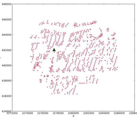
Figure 1.4 shows a map with the source locations for VSP1 (blue) overlaid with the source locations for VSP2 (red). The green triangle shows the location of the VSP well. An observation one can make from this figure is that most of the shot locations are really close to one another, and some other shot locations present differences in positioning from one survey to the other. An analysis of the difference in the source locations for both surveys and how it influence the repeatability will be shown in chapter 4.
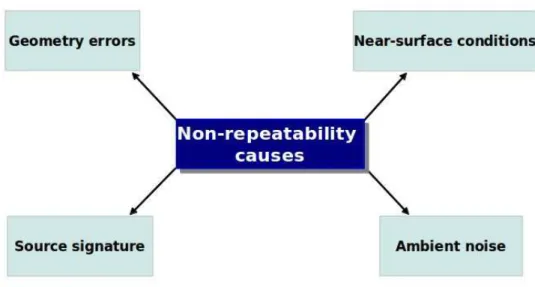
1.3 Non-repeatability causes
Repeatability of 4D land seismic data is affected by several factors. The most significant of them are: source and receiver geometry inaccuracies, differences in seismic sources signatures, variations in the immediate near surface and ambient non-repeatable noise (Pevzner et al. (2011), Jervis et al. (2012), Al Jabri (2011)). These factors are shown in Figure 1.5.
In order to accurately detect small changes due to production and injection effects within the reservoir, the sources and receivers of time-lapse multicomponent VSP surveys must be
Figure 1.4: Source locations for VSP1 (blue) overlaid with the source locations for VSP2 (red). The green triangle shows the position of the VSP well.
located exactly at the same positions. However, in practice, the source locations and the receiver orientations, if the array is not permanent, can vary from one survey to another survey. Repeatability of the acquisition geometry is very important for time-lapse studies, in order to resolve only time-lapse effects (Oghenekohwo & Herrmann, 2013). By analyzing the shotpoints for both surveys in the map (Figure 1.4), it is observed that some shot locations are really close to one another and other shot locations present differences in positioning from one survey to the other. This geometry provides data to study how repeatability can be improved by increasing the positioning accuracy of the source locations. This study is shown in chapter 4.
Since the two VSP surveys used permanent borehole arrays, the receiver geometry will not influence the repeatability of these data. The permanent array can provide data of sufficient quality to be applied to the task of time-lapse reservoir monitoring (Cornish et al., 2000).
In chapter 4, some errors in receiver orientation will be simulated in order to investigate how repeatability is affected by errors that may be generated when the borehole array is not permanent.
Propagation of the seismic waves through the near-surface layer may severely degrade seismic data quality, which is of particular importance in the interpretation of multicom-ponent seismic data (Zeng & MacBeth, 1996). Because of this, changes in near-surface conditions could be very important for repeatability of time-lapse surveys. In this case, the near-surface conditions varied from survey-to-survey, due to changes in soil saturation. When the first survey was acquired, the soil was wet, while when the second survey was acquired the soil was dry. The focus of this near-surface study will be on factors that can influence the repeatability of the land seismic data. It is expected that the attenuation and also the velocity of seismic waves in both surveys should be different due to these changes in the near-surface conditions. Time-shift maps, and amplitude spectral ratio maps will be estimated for both surveys to quantify the relative contribution of this factor into the overall non-repeatability of 4D surveys.
The VSP method of seismic data acquisition is a well-known technology whose advantage over surface data with regard to signal-to-noise and resolution near the borehole is generally accepted. It is expected to have less ambient noise affecting VSP data because the geo-phones are buried. Therefore, the ambient noise present in VSP data usually comes from the source. In this project, the ambient noise will be analyzed using signal-to-noise ratio attribute sections.
Andorsen & Landro (2000) found that there is a strong correlation between variations in the source signatures and lack of repeatability in the VSP data. The lack of repeatability of source signature is largely caused by the near surface being excited beyond its elastic limits, resulting in permanent, inelastic changes. These permanent changes may be credited to changes in absorption, which causes a constant phase delay, and/or changes in cohesive structure, which causes a constant time delay (Aritman, 2001). An analysis of how
repeata-bility can be affected by differences in source signatures is not done in this project and is left as a recommendation for future work.
Figure 1.5: Factors that can cause non-repeatability in land seismic data.
1.4 Motivation and objectives
4D technology is making dramatic advances in our ability to manage fields and increase their value. The sensitivity of 4D monitoring depends upon data repeatability. The more closely data are repeated, the smaller the reservoir changes we can diagnose. The smaller the production-related changes we can diagnose and recognize as deviations from model prediction, the earlier we have warning that our predictive model is in error and the earlier we can take corrective action and have greater impact upon field management (Calvert, 2005). Therefore, by increasing repeatability it is possible to improve the time-lapse seismic technology as a reservoir management tool.
The objective of this onshore repeatability study is to quantify the relative contribution of each factor that can affect the repeatability in a land seismic data. The factors analyzed in this study are: source and receiver geometry inaccuracies, variations in the immediate near surface and ambient non-repeatable noise. Understanding the factors that affect repeatability in time-lapse seismic projects can give insight into which factors are dominant and how they
can be mitigated (Jervis et al., 2012). 4D seismic data with higher repeatability can be more sensitive to small changes within the reservoir related to production and injection effects that can make a significant impact by enabling better field production diagnoses and by improving the field performance with less risk. Another goal of this project is to understand the advantages and disadvantages in the use of different repeatability metrics, normalized-root-mean-square (NRMS) difference and signal-to-distortion ratio (SDR) attribute, to evaluate the level of seismic repeatability between successive time-lapse seismic surveys.
1.5 Software used
To achieve the goal of this project, firstly it was necessary to do some processing in the data that will be explained in chapter 2. This 3D VSP processing was performed in Landmarks commercial software, Promax 3D. To calculate the repeatability metrics and the signal-to-noise ratio attribute and to plot all the maps shown in this thesis, Madagascar, Scilab and Python languages were used. Programs were also made to calculate variograms that are shown in chapter 4 using BrOffice Calc.
CHAPTER 2
SEISMIC PROCESSING STEPS AND PRELIMINARY REPEATABILITY ANALYSIS
To achieve the goal of this project, firstly it was necessary to process the data. Since the objective of this project is related to understanding factors that can affect repeatability in land seismic data, it was not necessary to do all the processing steps usually applied for imaging purposes. Both 3D VSPs were processed using the same sequences and parameters to exclude the effect of different processing steps in the repeatability analysis.
After geometry assignment, the tool was oriented to conform every receiver to one global coordinate system. The receivers were additionally inclined toward the incident downgoing wave in order to constrain the energy of downgoing compressional waves on one component and shear waves on a plane (Michaud, 2001). Cross-correlation was used to indicate which receivers were too noisy and should not be taken into account in the repeatability analysis. All the processing steps shown in this chapter were performed with the ProMax (Land-mark, Halliburton) processing software system.
In this chapter, a preliminary analysis of the repeatability in the VSP data is conducted in both time and frequency domain. Seismic repeatability is critically important in order to determine the level of confidence in the interpretation of any seismic changes related to production or injection effects. On land, non-repeatability effects are produced by differences in the acquisition geometry, variations in the near surface conditions, differences in the source signature and ambient noise. The analysis conducted in this chapter is made in a general way. Repeatability metrics are not used in order to quantify the non-repeatability in the raw data and there is no attempt in correlate any of the non-repeatable events found with the factors that can cause non-repeatability in land seismic data. The analysis including the repeatability metrics are shown in chapter 3 and the analysis including correlation with these factors are made in chapters 4 and 5.
2.1 Geometry assignment and first break picking
In this processing step, firstly some tables in the database were filled with survey infor-mation as positions of the sources and the receivers, charge and depth of the sources and grid informations. Then, this information was loaded in the header of the traces.
First breaks were also picked in this step. First break is the time of the first arrival or the time when the direct P-wave hits the geophone. The quality control of the 3D VSP geometry involves observing first break picks. First break picks were also used in the processing step explained below.
2.2 Tool orientation
3D multicomponent VSP data are recorded with receivers made of three mutually or-thogonal geophones. One geophone is oriented toward the vertical direction, whereas the two others are free to orient toward any arbitrary direction in the horizontal plane (Michaud, 2001). The vertical component direction is downward and the horizontal components az-imuths are randomly oriented. Because of this, from one receiver level to another, the two horizontal components can be oriented differently.
It is necessary to remove the effect of the different receiver orientations in order to com-pare data recorded at different levels or at different tool positions. This correction involves rotating the data to a global coordinate system, common for all receivers (Michaud, 2001). The chosen coordinate system is radial relative to the shot point. The orientation process is performed using the direct P-wave polarization plane method. This method assumes that P-wave energy is linearly polarized in the radial direction given by source and receiver coordinates.
The VSP data are rotated in the horizontal plane to orient one horizontal component with the source-receiver direction, often referred to as the horizontal radial component, and the other component orthogonal is referred to as the transverse component (Kuzmiski et al., 2009). The receiver is oriented by rotating the horizontal components about the vertical axis,
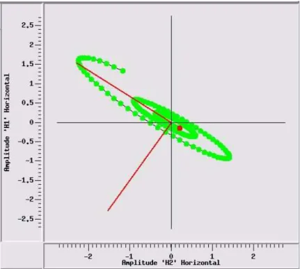
until the energy of the first compressional arrival is maximized on one horizontal component. This processing step is made based on hodogram analysis. A hodogram represents particle motion in 2-D (Figure 2.2). Hodogram analysis (Hinds et al., 1996) performed on the first break wavelets of the two horizontal datasets (from the same source location) is used to polarize the x and y data onto two principal axes that are normal (transverse) and tangential (radial) to the plane defined by the source and the well. The hodogram usually resembles an ellipse pointing in the direction of the azimuth of the downgoing wave (Figure 2.2). The hodogram method polarizes the horizontal axis data using the downgoing P-wave energy in the first break wavelet. A time window around the first break of 16 ms was selected, and the data from the two horizontal channels were plotted on an orthogonal axis. The angle found in the hodogram analysis is used to calculate the real orientation of the horizontal components and also to calculate the radial and transverse component traces.
Just a few shots around the wellbore with offsets less than 1000 ft were used in order to avoid the influence of lateral refraction in the estimation of the real orientation of the horizontal components. The angle for the real orientation of the horizontal components is given by the subtraction of the known source azimuth by the maximum signal polarization direction found using the hodogram analysis. The computed angle of actual orientation for each geophone is given by the average of the angles found for all these few shots (Lubis, 2012). The estimated angle of the tool orientation is then applied to the corresponding receiver on both horizontal components.
The calculus of the orientation angles is made for VSP 1. However, since the geophones are permanently installed the orientation of the horizontal components are the same for VSP 1 and for VSP 2. Therefore, the same orientation angles found for VSP 1 are applied for VSP 2.
After tool orientation, one of the horizontal components is rotated to the source-receiver direction or to the direction of maximum signal polarization. This rotation produces three output wavefields: vertical, transverse and radial. In the vertical component, the particle
motion is confined to the plane of the source-receiver pair and in the direction of propaga-tion. In the radial component, the particle motion is transverse to the direction of wave propagation and in the plane of the source-receiver pair. In the transverse component, the particle motion is orthogonal to the radial component. The P-wave source was expected to produce a strong vertical component and a strongly SV-wave oriented to the radial compo-nent. Energy on the transverse component was expected to be minimized (Cornish et al., 2000). Therefore, the energy created by the compressional wave source is mainly recorded by vertical and radial components. The transverse component contains polarized SH waves as well as out-of-plane reflections and the vertical and radial components contain combined downgoing and upgoing P and SV waves.
Figure 2.3 shows the same shot shown on Figure 2.1 after tool orientation. This record from left to the right corresponds respectively to: vertical, transverse and radial components. A first observation one can make from this figure is that there is little energy in the transverse component. This energy can be related to anisotropy, heterogeneities or random noise. As expected, the vertical and the radial components contain the main energy created by the explosive source.
2.3 Rotation to the maximum P-wave
The goal of this research is to understand factors that can affect repeatability in land seismic data. Because of this, in some of the repeatability analyses only the direct downgoing P wave will be used since it is the least contaminated from other waves and has higher signal-to-noise ratio. Moreover, the downgoing waveform in VSP data provides reliable information about the evolution and attenuation of the seismic wavelet.
In the acquisition of these surveys, explosive sources and three component geophones were used in order to emphasize P- and converted S-waves. As stated by Yang et al. (2007), when the media around the shot point is isotropic, and the the vibrations generated by the source are the same in various directions, then pure P-waves are produced. In practice, it is impossible for the dynamite and surrounding media to satisfy all of the conditions and both
Figure 2.1: Raw data. These data were recorded with receivers made of three mutually orthogonal geophones. The figure is showing the three components of the data before any rotation. The record on the left corresponds to the vertical component, and the records in the middle and on the right correspond to the horizontal components, that can be pointing to any random direction in the raw data.
P- and S-waves are produced. The intensity of the generated downgoing S-waves depends on the characteristics of the dynamite and surrounding media.
Previous studies show that this kind of wave source generates relatively strong pure P-waves and weaker pure S-P-waves. Downgoing S-P-waves observed at zero offset can be divided into two categories: pure waves produced near the source and downgoing converted S-waves produced when P-S-waves are transmitted at a high Poisson’s ratio interface. Yang et al. (2007) states that the main frequency of pure S-wave is usually lower than the pure P-waves while the main frequency of a downgoing converted wave is close to that of a P-wave. The first rotation was performed on the horizontal plane to orient one horizontal nent with the source-receiver direction (maximum energy) and the other horizontal compo-nent orthogonal to this (minimum energy). In order to isolate the downgoing P-wave events in one component, and the downgoing S-wave events in another component, another rotation
Figure 2.2: Hodogram analysis. The data in a window around the first break from the two horizontal channels are plotted on an orthogonal axis. The hodogram usually resembles an ellipse pointing in the direction of the azimuth of the downgoing wave.
is necessary. In this rotation, the receivers are inclined toward the incident downgoing wave in order to constrain the energy of compressional (P-) waves on one component and shear (S-) waves on a plane.
This processing step is also based on hodogram analysis. In this case, the rotation angles used for the polarization are found using a hodogram analysis of the vertical and radial components input data.
This rotation produces three output wavefields: P, SV and SH. P- and SV- waves in an isotropic medium are aligned toward the source; one component contains all the downgoing P wave energy and the other component contains the downgoing SV- energy. The up-going P and SV wave-fields exist mixed on both of these components (Kuzmiski et al., 2009). Figure 2.4 shows the record for the same shot shown in Figure 2.1 and Figure 2.3 after the second rotation. As can be seen in this figure, downgoing P-wave events are isolated in the component on the left, that from now on will be called component 1, and the downgoing
Figure 2.3: Data after tool orientation. This record from left to right corresponds respectively to: vertical, transverse and radial components. The transverse component contains polarized SH-energy as well as out of plane reflections and the vertical and radial components contain combined P- and SV- energy.
SV-wave events are present mainly in the component on the right that from now on will be called component 2. After a visual inspection of some shots, it was possible to see that the downgoing transmitted P and S-waves begin to refract at the shallower receivers as offset increases. In all the following analyses just the components 1 and 2 are used. The transverse component is not used in the studies presented in this thesis.
Figure 2.5 shows the data after this second rotation, highlighting that the P-wave down-going energy is constrained in one component (left) and the downdown-going S-wave energy is constrained in another component (right). The frequency of the downgoing S-waves is ob-viously lower than that of the downgoing P-waves. Since downgoing converted S-waves pro-duced when P-waves are transmitted at a high Poisson’s ratio interface should have primary frequency similar to the transmitted P-wave, the downgoing S-wave shown in Figure 2.4 and Figure 2.5 should be pure S-waves produced at the source.
Figure 2.4: Data after second rotation. The downgoing P-wave was maximized in one component. The record in the left shows the component in which the downgoing P-wave was maximized, the record in the middle contains polarized SH-energy and the record in the right contains maximized downgoing S-wave.
Figure 2.5: Data after second rotation. The yellow and blue circles in the figures are high-lighting the downgoing P-wave and the downgoing S-wave, respectively.
2.4 First break picking
After the second rotation, the first break was picked in the data, in the component that contained the downgoing P-wave. These picks were made just for some receivers (4, 6, 12 and 18) and all shots. These picks were made visually, without using any automatic process. Later, these first break picks were used to compute the time-shift maps for some receivers, as explained below. Figure 2.6 shows two shots with the first break picked.
Figure 2.6: First break pick. All the picks were made in a visual way without using any automatic process.
2.5 Cross correlation
The cross-correlation between the traces of survey 1 and survey 2, for each shot, was used to analyze the receivers that presented good repeatability. In another words, cross-correlation was used to help choose some receivers that had a low signal to noise ratio and because of this were not included in the repeatability analysis.
Cross-correlation analysis was made for all the shots. Figure 2.7 shows the result of the cross-correlation for one shot. The result showed that the three shallower receivers have a poor correlation for almost all the shots. Therefore, these three shallow receivers will not be taken into account in the following repeatability analysis.
Figure 2.7: Cross- correlation between corresponding traces of a shot from VSP 1 and of a shot from VSP2. This cross-correlation shows that the three shallower receivers were noisy and should not be taken into account in the following analysis.
2.6 Preliminary repeatability analysis in time-domain
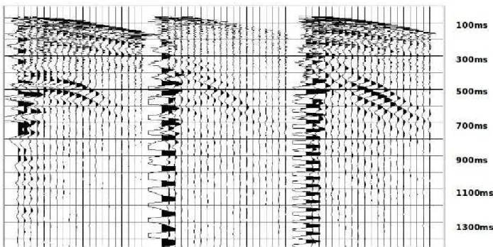
To better understand the behavior of these data related to repeatability, firstly I plotted the near-offset shot from survey 1, with the first near-offset shot from survey 2 and the difference between them (Figure 2.8). This difference was computed as a direct subtraction (sample by sample) of the monitor 1 shot gather and the monitor 2 shot gather.
As can be seen in Figure 2.8, the difference between these two shots is remarkable which implies that there is significant non-repeatability between the raw data from both surveys that may be caused by some of the factors that can influence repeatability in land seismic data, such as source positioning errors, differences in seismic source signatures, near surface conditions and ambient noise.
There are several techiniques available to enhance the repeatability between successive surveys in time-lapse projects. One of them is related to correct time-shifts, bandwidth and phase using a cross-equalization process. A commonly used method for equalizing two seismic surveys is composed of the following steps (Cheng et al., 2009):
• (1) First break time alignment: align the first break of the repeat survey with the baseline.
Figure 2.8: Near-offset shot from survey 1 on the left, from survey 2 in the middle and the difference between them on the right. This shows a remarkable difference between these two shots that may be caused by factors shown in Figure 1.5
• (2) Match-filtering: The spectrum of the repeat survey is matched to the baseline survey inside a specific window by the use of the Wiener-Levinsion algorithm.
• (3) Gain equalization: A global gain equalization is then applied to both data sets. These processes used to enhance the repeatability between successive surveys are not applied to the data in this thesis because the main purpose of this research is related to evaluate the level of seismic repeatability in the raw data at Delhi Field and to understand the factors that can cause non-repeatability in land seismic data.
After this first analysis, I plotted a seismogram with traces from survey 1 and survey 2 merged for the near offset shot. The objective of this plot is to show if there are phase and amplitude differences between traces from datasets from surveys 1 and 2. Figure 2.9 shows this seismogram.
By analyzing Figure 2.9, I noted a slight difference in the amplitude between traces from both surveys. A time-shift between traces from both surveys can also be observed. Differences in phase are not observed for this shot.
Figure 2.9: Traces from the near-offset shot from survey 1 and survey 2 side by side. This seismogram is plotted in order to emphasize the amplitude and phase differences between the two shots. It also shows a time shift between traces from one survey to the other.
Time shifts are frequently observed between the surveys that comprise a time-lapse seis-mic dataset. The timing differences may be consistent, caused, for example, by different acquisition reference time definitions or by differences in the near surface conditions when the two surveys were acquired, or they may vary from line to line or shot to shot, perhaps as a result of variable source timing and geometry errors.
Time-shifts between the two surveys were estimated for some receivers and all the shots. The picks were made in the first arrivals in component 1 for both surveys. Then, these picks were subtracted from each other for corresponding traces from both surveys to compute the time-shift maps. Time-shift maps were generated for some receivers (4, 12 and 18). Figure 2.10 shows the time-shift map for receiver 12. The time-shift maps for receivers 4 and 18 are shown in chapter 5.
Figure 2.10 shows that the presence of time-shifts in the data between survey 1 and survey 2 are remarkable. The red color in the map corresponds to positive time shifts and the blue color in the map corresponds to negative time-shifts. Since these maps were generated as the values for the first break picks for survey 1 minus the values for the first break picks for
survey 2, positive time-shifts imply that the first break time for survey 1 is greater than the first break time for survey 2, and negative time-shifts imply the opposite.
As stated before, no process was used to equalize both data. The time-shift map shows punctual events that can probably be related to variable source timing between both surveys or to errors in the acquisition geometry. In general, time-shifts are positive in the north part of the map and negative or zero in the bottom part of the map. The discussions about the factors that can be causing these time-shifts and also the consistency of the time-shift maps for different receivers are made in chapters 4 and 5, respectively.
Figure 2.10: Time-shift map for receiver 12. These maps were generated as the values for the first break picks for survey 1 minus the values for the first break picks for survey 2. Positive time-shifts (red) imply that the first break time for survey 1 is greater than the first break time for survey 2, and negative time-shifts (blue) imply the opposite.
2.7 Preliminary repeatability analysis in frequency-domain
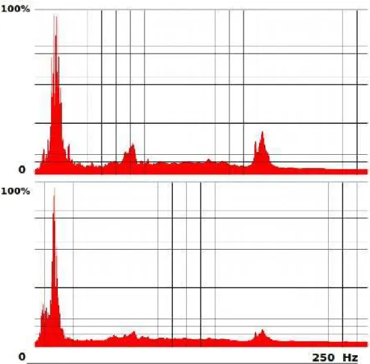
amplitude spectra of some shots from both surveys. This analysis was made for component 1 and for component 2. Figure 2.11 and Figure 2.12 are showing the frequency spectrum for survey 1 and for survey 2, for both components 1 and 2, respectively.
Figure 2.11: Frequency spectrum for component 1 of one shot from survey 1 on the top, and frequency spectrum for the same shot from survey 2, on the bottom. This figure shows that the frequency spectrum for the component 1 from survey 2 is more attenuated than the frequency spectrum for component 1 from survey 1.
A first observation one can make from these amplitude spectra plots is that the frequency content is different for both surveys, especially for component 1. The frequency spectrum for the shot from survey 2 is more attenuated than the frequency spectrum for the same shot from survey 1. For this shot, this difference is larger for the first component (Figure 2.11) than for the second component (Figure 2.12). This analysis was made for several shots,
Figure 2.12: Frequency spectrum for component 2 of one shot from survey 1 on the top, and frequency spectrum for the same shot from survey 2, on the bottom. This figure shows that the frequency spectrum for the component 2 from survey 2 is slightly more attenuated than the frequency spectrum for component 2 from survey 1.
and most of them showed the same behavior, the frequency content was less attenuated for survey 1 than for survey 2, specially for component 1.
Changes in the frequency spectrum may be related to some factors as, for example, ambient noise and with differences in the near-surface conditions. In this case, when the first survey was acquired the soil was wet, while when the second survey was acquired the soil was dry. According to Al Jabri (2011), it is reasonable to assume that the principal cause of non-repeatability issues in land seismic data is related to temporal variations of the near surface conditions. He showed that the change in water saturation of the near surface
can cause changes in velocity and attenuation and that the wet near surface can provide better seismic energy transmission and a broader signal compared to the dry near surface. Pevzner et al. (2011) also observed a much lower signal level during dry periods compared to wet periods. In this case, the same behaviour was observed for the amplitude spectra from both surveys, the data collected during the wet season (survey 1), had higher frequency content than the data collected during the dry season (survey 2) for most of the shots. This discussion continues in chapter 5.
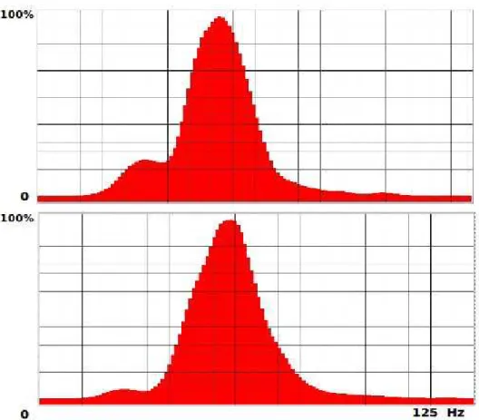
It is known that upgoing P- and S- waves are presented in components 1 and 2 of the data. To better understand what causes component 1 to have a higher difference in the amplitude spectra compared to component 2, the frequency spectrum was plotted for component 1 for both surveys with a window around the downgoing P-waves, and for component 2 with a window around the downgoing S-waves. In this way, it is ensured that the main information in the frequency spectrum comes from P and from S-waves separately. Figure 2.13 and Figure 2.14 show the frequency spectrum for survey 1 and for survey 2 with the time-window applied, for both components 1 and 2, respectively.
By analyzing the frequency spectrum with the time-window applied around the downgo-ing P-waves for component 1, it is possible to observe that component 1 of the receivers is strongly dependent on water saturation. The frequency spectrum for survey 1 is remarkably less attenuated than the frequency spectrum for survey 2. On the other hand, the frequency spectrum with the time-window applied around the downgoing S-waves for component 2, shows a weak dependency on water saturation. It is expected since, as stated by Mavko et al. (2005), some laboratory and field data (albeit very sparse) indicate that the S-wave attenuation in a sediment sample weakly depends on water saturation.
Figure 2.13: Frequency spectrum for component 1 of one shot with a window around the downgoing P-wave from survey 1 on the top, and frequency spectrum for the same shot from survey 2, on the bottom. This figure shows that, for this shot, the amplitude spectrum for component 1 from survey 2 is remarkably more attenuated than the amplitude spectrum for component 1 from survey 1.
Figure 2.14: Frequency spectrum for component 2 of one shot with a window around the downgoing S-wave from survey 1 on the top, and frequency spectrum for the same shot from survey 2, on the bottom. This figure shows that, for this shot, the difference between the amplitude spectrum for component 2 from survey 1 and the amplitude spectrum for component 2 from survey 2 is remarkably less than the differences found for component 1.
CHAPTER 3
REPEATABILITY METRICS
One of the critical limitations encountered in time-lapse seismic projects is the degree of repeatability between successive surveys. Repeatability is a measure of the similarity of the seismic response between two seismic surveys excluding production-related effects (Li et al., 2004). The confidence level in interpretation of time-lapse events is directly related to the attained repeatability.
Kragh and Christie (Kragh & Christie, 2002) presented a paper on repeatability, normalized-root-mean-square (NRMS), and predictability (PRED) in 2001. Since then, NRMS and predictability have been the most widely used metrics for analyzing 4D noise in time-lapse studies. In papers related to 4D projects, NRMS is still the most used repeatability metric. In 2011 and 2012, Juan Cantillo (Cantillo (2011) and Cantillo (2012)) presented a different way to estimate time-lapse repeatability from the perspective of perturbation theory. He introduced the signal-to-distortion ratio (SDR) attribute as a reliable indicator of time-lapse repeatability.
In this project, to evaluate repeatability of the two surveys, two different metrics were computed: normalized-root-mean-square (NRMS) that measures the difference between two surveys, and the signal-to-distortion ratio (SDR) attribute that uses the cross-correlation be-tween corresponding pairs of traces from different surveys. The advantages and disadvantages of these repeatability metrics are discussed in this chapter. Results of these repeatability metrics applied on component 1 and on component 2 of the Delhi multicomponent VSP data are also shown in this chapter.
3.1 NMRS difference
between two corresponding traces from successive surveys divided by the average RMS of the inputs. It is expressed as a percentage. Normalized-root-mean-square difference is computed using the following equation (Kragh & Christie, 2002):
N RM S = 200 RM S(a − b)
RM S(a) + RMS(b)% (3.1)
where a and b are the two input data, and the RMS operator is defined as:
RM S = p( P x
2
)
N (3.2)
where N is the number of samples in the window.
For NRMS, lower values generally correspond to better repeatability and higher values to less repeatability. In another words, when NRMS increases the repeatability decreases and vice versa. The values of NRMS are not intuitive and are not limited to the range 0-100%. As stated in Kragh & Christie (2002), for example, if both traces contain random noise, the NRMS value is 141% (√2). If both traces anti-correlate (i.e., 180o out of phase, or if one
trace contains only zeros) the NRMS value is 200%, the theoretical maximum. If one trace is half the amplitude of the other, the NRMS value is 66.7%.
NRMS difference is affected by even small changes in the data. It is sensitive to overall phase, amplitude and time-shift differences. Because of this, the comparison of a trace with the same trace just with a static shift, can give the same NRMS value as the comparison of two traces with different shapes.
From Cantillo (2012), NRMS difference values in the range from 0% to 10% indicate excellent repeatability. Values in the range from 11% to 25% are considered good repeata-bility and in the range from 26% to 50% fair repeatarepeata-bility. From 51% to 200% the data are considered to have poor repeatability. These values are just approximations to give the reader insights about what to expect concerning repeatability for different NRMS values.
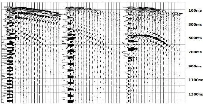
To evaluate the repeatability of survey 1 and survey 2, NRMS difference sections were computed for some shots. This calculation was made using a sliding window of 100ms. The NRMS sections were smoothed using a Gaussian filter. Figure 3.1 shows a NRMS section
for component 1 of shot 1600547 and Figure 3.2 shows the seismograms for component 1 of this shot for survey 1 and for survey 2 side by side.
Figure 3.1: NRMS difference section for component 1 of shot 1600547. The lower values (blue) are related to higher repeatability, while the higher values (red) are related to lower repeatability.
Figure 3.2: Seismograms of component 1 of shot 1600547. On the left is the record for survey 1 and on the right is the record for survey 2.
The first observation one can make of the NRMS section shown in Figure 3.1, is that, in general, the repeatability is higher for the smaller times and is lower for the greater times. The low repeatability that occurs in the time window from 0 to 0.1s is related to the fact that until this time no signal arrived in the geophones and this region presents just random noise, as seen in Figure 3.2. Ambient noise ocurring just before the first-breaks is related to the lowest signal-to-noise ratio and is not repeatable. The fact that the repeatability is higher for the smaller times and lower for the greater times should also be related to the S/N ratio. As the wave travels in the medium, the signal is attenuated and the signal to noise ratio decreases.
NRMS difference measures the relative difference between two seismic traces. Typical values for modern 4D surveys are 0.1 to 0.4, which represent an ability to reproduce seismic amplitudes to within 10-40% in the final stacked data (Miller & Helgerud, 2009). Houck (2007) states that recently, surveys with average NRMS difference of less than 20% have become common, and cases have been reported where NRMS values below 10% have been observed. Wu et al. (2011) showed that for their time-lapse 3D VSP project using a perma-nent array a repeatability of 20% was achieved within a range of 1500m around the VSP well. All these cases are related to data that are already processed and with cross-equalization techniques applied. In order to retain the inherent effect caused by each factor that affects repeatability on 4D land seismic data, no matching technique was applied to the data. Be-cause of this, the values I found for the NRMS difference in this section are relatively high compared to the values in the literature that are usually calculated for the processed data with cross-equalization processes applied.
The next step was to generate a map of the NRMS values that provides spatial informa-tion about the repeatability. NRMS values were calculated for a window of 200ms around the direct downgoing wave. Only the direct downgoing wave was used to generate the maps of repeatability metrics because it is the least contaminated from other waves and has higher signal-to-noise ratio. Figure 3.3 shows this NRMS map.