ANALYSIS OF INTELLIGENT COMPACTION FIELD DATA ON LAYERED SOIL
by Aaron M. Neff
ii
A thesis submitted to the Faculty and the Board of Trustees of the Colorado School of Mines in partial fulfillment of the requirements for the degree of Master of Science
(Engineering) Golden, Colorado Date ________________________ Signed:______________________________ Aaron M. Neff Signed:______________________________ Dr. Judith C. Wang Thesis Advisor Signed:______________________________ Dr. Michael A. Mooney Thesis Advisor Golden, Colorado Date ________________________ Signed:______________________________ Dr. John E. McCray Department Head and Professor Civil and Environmental Engineering
iii ABSTRACT
Intelligent compaction (IC) procedures have been gaining popularity as a way to measure mechanistic soil material properties (e.g. stiffness) during the compaction process for earthwork projects. IC procedures involve the interpretation of roller measured soil stiffness from vibratory roller drum accelerations and offer an advantage over current spot testing methods, as IC
provides real-time continuous feedback during the compaction process and 100% test coverage of the earthwork site.
The objective of this study is to provide the first detailed analysis of IC field data from vibratory roller compaction of layered soil systems. The interpretation of roller measured soil stiffness is currently ambiguous for two main reasons: (1) IC vibratory rollers provide a
composite measure of soil stiffness in layered earthwork situations and (2) roller measured soil stiffness from edge mounted (EM) accelerometers can vary significantly due to rocking motion of the drum. To investigate these issues, left and right EM acceleration data from a vibratory roller are used to compute a composite roller measured soil stiffness at the center of gravity (CG) of the drum. CG soil stiffness, which is not subject to the variations associated with drum
rocking, are used to evaluate data from two field sites with multiple 15 – 30 cm thick base/subbase/subgrade lifts to investigate their sensitivities to variable lift materials and thicknesses. CG soil stiffness increases with the addition of subbase and base lifts, showing sensitivity to changes in soil materials. CG soil stiffness also increases with the addition of multiple base lifts, showing sensitivity to an increase in the overall thickness of the base material. CG soil stiffness is not sensitive to small variations in the subbase and base lift thicknesses, showing CG soil stiffness is sensitive to the addition of 15 – 30 cm thick subbase and base lifts but not the small variations in lift thickness associated with each of these lifts.
iv TABLE OF CONTENTS ABSTRACT ... iii LIST OF FIGURES ... vi LIST OF TABLES ... ix CHAPTER 1 INTRODUCTION ...1
1.1 Motivation for Work ... 2
1.2 Summary ... 5
CHAPTER 2 LITERATURE REVIEW ...7
2.1 Roller Measured Values ... 7
2.2 Intelligent Compaction Specifications ... 9
2.3 Roller Measurement Depth ... 11
2.4 Roller Modes of Operation ... 13
2.5 Dependence of Roller Measured Values ... 14
2.6 Influence of Rocking Motion ... 16
2.7 Research Potential ... 22
CHAPTER 3 ANALYSIS OF CENTER OF GRAVITY ROLLER DRUM VIBRATION AND RESULTANT SOIL STIFFNESS ON COMPACTED LAYERED EARTHWORK ...24
3.1 Field Data ... 26
3.1.1 Florida Earthwork Site ... 26
3.1.2 North Carolina Earthwork Site ... 27
3.2 Roller Instrumentation and Center of Gravity Soil Stiffness ... 28
3.3 Analysis of Florida Data ... 32
3.4 Analysis of North Carolina Data ... 40
3.5 Summary of Florida and North Carolina Sites ... 42
v
4.1 Conclusions ... 44
4.2 Recommendations for Future Research ... 45
LIST OF ACRONYMS, ABBREVIATIONS, AND SYMBOLS ...46
REFERENCES CITED ...49
APPENDIX A SUPPLEMENTAL ROCKING ANALYSIS ...52
APPENDIX B SUPPLEMENTAL DATA AVERAGING ANALYSIS ...56
vi
LIST OF FIGURES
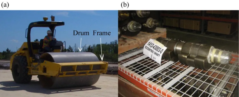
Figure 1.1 Components of smooth drum vibratory rollers showing: (a) drum and frame of the roller; (b) eccentric masses located inside the drum of the roller (pictures obtained from
the Colorado School of Mines bb149 drive) ...4
Figure 2.1 Free body diagram of forces acting on the vibratory roller (from Mooney and Rinehart 2009) ...9
Figure 2.2 (a) force-displacement loop during contact mode; (b) force-displacement loop during partial loss of contact mode (from Mooney and Facas 2012) ...10
Figure 2.3 Measurement depth of intelligent compaction rollers and spot tests (from Mooney and Facas 2012) ...12
Figure 2.4 3DOF lumped parameter model (from van Susante and Mooney 2008) ...14
Figure 2.5 Differences in soil stiffness with driving direction (from Facas 2010) ...16
Figure 2.6 Lumped parameter rocking model (from Facas et al. 2010) ...17
Figure 2.7 Influence of sensor position on drum acceleration and roller measured stiffness: (a) five soil stiffness profiles each with five discrete ks,a; (b) peak drum acceleration as a function of sensor position; and (c) computed ks-R as a function of sensor location (from Facas 2010) ...19
Figure 2.8 Directional dependence of EM MV and CG MV (from Facas 2010) ...21
Figure 3.1 Florida and North Carolina earthwork sites: (a) Plan view of Florida site; (b) Elevation view of lift materials and nominal lift thicknesses for the Florida site; (c) Plan view of North Carolina site; (d) Elevation view of lift materials and nominal lift thicknesses for the North Carolina site ...28
Figure 3.2 Force-displacement loops on the S lift at the North Carolina site showing roller measured soil stiffness, ks ...29
Figure 3.3 Difference in ks from instrumentation on the left and right sides of the drum ...30
Figure 3.4 ks-CG for the EF lift ...32
Figure 3.5 Comparison of center of drum travel path for EF and S lifts; circled region indicates the area over which IC data is compared. ...33
Figure 3.6 Comparison of EF and S lift from x = 35 – 75 m in lane 1: (a) S lift thickness, hs; (b) EF and S ks-CG; (c) percent change in ks-CG from EF to S; (d) force-displacement loops ...34
Figure 3.7 Comparison of S and SS lifts from x = 35 – 65 m in lane 2: (a) SS lift thickness, hss; (b) S and SS ks-CG; (c) percent change in ks-CG from S to SS; (d) force-displacement loops ...35
vii
Figure 3.8 Comparison of SS and B1 lifts from x = 55 – 75 m in lane 3: (a) B1 lift thickness,
hB1; (b) SS and B1 ks-CG; (c) percent change in ks-CG from SS to B1; (d) force-displacement
loops ...36
Figure 3.9 Comparison of B1 and B2 lifts from x = 35 – 51 m in lane 3: (a) B2 lift thickness, hB2; (b) B1 and B2 ks-CG; (c) percent change in ks-CG from B1 to B2; (d) force-displacement loops ...37
Figure 3.10 Comparison of B2 and B3 lifts from x = 55 – 75 m in lane 1: (a) B3 lift thickness, hB3; (b) B2 and B3 ks-CG; (c) percent change in ks-CG from B2 to B3; (d) force-displacement loops ...39
Figure 3.11 Comparison of B3 and B4 lifts from x = 55 – 75 m in lane 4: (a) B4 lift thickness, hB4; (b) B3 and B4 ks-CG; (c) percent change in ks-CG from B3 to B4; (d) force- displacement loops ...40
Figure 3.12 Comparison of S, B1, and B2 showing: (a) B1 lift thickness, hB1; (b) percent change in ks-CG from S to B1; (c) B2 lift thickness, hB2; (d) percent change in ks-CG from B1 to B2; (e) S, B1, and B2 ks-CG; (f) force-displacement loops ...41
Figure 3.13 Summary of Florida and North Carolina earthwork sites: (a) Force-displacement loops for the Florida site; (b) sensitivity of ks-CG to htotal and corresponding ks-CG valuesfor Florida site; (c) sensitivity of ks-CG to htotal and corresponding ks-CG values for North Carolina site ...43
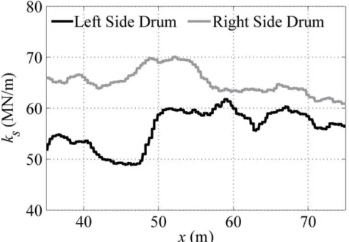
Figure A-1 (a) Left side drum; (b) CG; and (c) right side drum peak drum acceleration from data collected on the EF lift at the Florida earthwork site ...52
Figure A-2 (a) Left side drum; (b) CG; and (c) right side drum soil stiffness from data collected on the EF lift at the Florida earthwork site ...53
Figure A-3 Rocking of the drum ...54
Figure B-1 Comparison of averaging lengths for the S lift, lane 2 data from the Florida earthwork site ...57
Figure C-1 Roller parameters on the EF lift, lane 5 from the Florida earthwork site: (a) ks-CG; (b) | ̈ | ; (c) zd-CG; (d) Fc-CG; (e) ϕCG ...59
Figure C-2 Comparison of EF and S lift over all overlapping x-y sections ...60
Figure C-3 Comparison of S and SS lifts over all overlapping x-y sections ...61
Figure C-4 Comparison of SS and B1 lifts over all overlapping x-y sections ...62
Figure C-5 Comparison of B1 and B2 lifts over all overlapping x-y sections ...63
viii
ix
LIST OF TABLES
Table 3.1 Summary of soils used at the Florida earthwork site ...27 Table 3.2 Summary of soils used at the North Carolina earthwork site ...28
1 CHAPTER 1 INTRODUCTION
The objective of this work is to present detailed experimental data from a variety of layered soil situations, exploring the sensitivity of roller response to the physical characteristics of the underlying soil system. Vibratory rollers are used in earthwork projects for soil
compaction. The dynamic behaviors of vibratory rollers change while the soil is being
compacted, and by monitoring the dynamic behavior of the roller, a measure of the underlying soils’ stiffness can be determined. The process of real-time monitoring and interpretation of dynamic vibratory roller behavior during compaction is known as intelligent compaction (IC) or continuous compaction control (CCC). Although these methods have been widely used in Europe since the 1970’s, the United States has only recently started using them (e.g. Petersen 2005; Camargo et al. 2006; Zambrano et al. 2006; Rahman et al. 2008; White et al. 2008; Mooney et al. 2010; Liu et al. 2011). IC methods have been widely researched (e.g. Anderegg and Kaufman 2004; Sandstrom and Pettersson 2004; Brandl et al. 2005; Mooney and Adam 2007; Mooney and Rinehart 2007); however, there are still ambiguities associated with their usage, including: (1) the effect of layered soils’ lift thicknesses and soil material types on the dynamic behavior of the roller and the associated roller measured soil stiffness values; and (2) an appropriate definition of roller measured soil stiffness that appropriately accounts for the effects of drum rocking, removing dependence on roller/sensor geometry. The following thesis presents the results of a study that addresses these two ambiguities through the analysis and interpretation of experimentally obtained IC data.
2 1.1 Motivation for Work
In traditional earthwork construction processes, lifts of fill soils are individually spread and compacted to design-specified dry density levels. Site designs typically require certain relative compaction measures are met, where the relative compaction of a fill layer is defined as the ratio of the in-situ dry density of a fill lift to the maximum dry density of the fill soil as determined by a laboratory Proctor test (ASTM D698-12 and ASTM D1557-12 provide standards for Standard Proctor tests and Modified Proctor tests, respectively). Increases in dry density measurements are assumed to be representative of increases in structural embankments’ stiffness and strength properties and are typically measured via spatially discrete spot testing techniques such as sand cone and nuclear density gauge measurements. In current quality assurance/quality control (QA/QC) procedures for compaction if, after a fill lift has been spread and compacted, the measured in-situ dry densities are found to be insufficient (i.e the relative compaction requirement is not met), the fill lift is recompacted, and spot tests are again taken to determine if the relative compaction requirement has been satisfied. If the measured in-situ dry densities are sufficient such that the relative compaction requirement has been met or exceeded, only then can the next fill layer be spread and compacted.
While generally effective, these traditional QA/QC methods of embankment compaction suffer from three major limitations: (1) they are based upon measures of dry density, which are roughly correlated with stiffness, and do not explicitly quantify measures of stiffness that can be used for mechanistic engineering analyses; (2) they are spatially discrete methods, usually covering less than 1% of the entire earthwork site; and (3) they are temporarily discrete methods that do not provide real-time, continuous feedback during the compaction process (Mooney and Adam 2007).
3
These three limitations have provided the impetus for the development of more advanced IC procedures, where mechanistic material properties may be quantified and monitored in a spatially and temporally continuous manner. The early use of IC, with respect to vibratory rollers, referred to the ability of the roller to automatically adjust the roller operating parameters (i.e. frequency of vibration and amplitude of vibration) during operation for optimal compaction metrics (Anderegg and Kaufmann 2004). IC now includes CCC, where QA/QC procedures can be performed in real time while the soil is being compacted (Sandstrom and Pettersson 2004). Using IC compaction results, soil stiffness properties can be monitored in real-time, while the soil is being compacted, providing 100% test coverage of the earthwork site (Anderegg et al. 2006, White et al. 2007, Liu et al. 2011). The use of IC not only provides a better benefit-to-cost ratio compared to current procedures but can also provide soil stiffness properties, which can be used to help predict the mechanical response of the structures supported by the compacted soils (Peterson et al. 2006; Zambrano et al. 2006).
Rollers used for soil compaction have vibratory drums that are more efficient at compacting the soil than the static weight of the roller alone (Facas 2010). Figure 1.1 shows a typical Sakai smooth drum vibratory roller and the different components of the roller. The drum of the vibratory roller contains rotating eccentric masses, typically rotating between 25-35 Hz, causing the drum to vibrate (Brandl et al. 2005, Mooney and Rinehart 2007, Facas 2010). Early research showed the dynamic behavior of the drum (i.e. drum acceleration) changed while the soil was compacted (Anderegg et al. 2006, Mooney and Adam 2007). By monitoring the dynamic time history of the acceleration of the drum during compaction, information about the compacted state of the soil and soil stiffness properties can be determined (Brandl et al. 2005). The soil stiffness is referred to as a roller measurement value (MV) (see section 2.1 for a detailed
4
discussion on roller MVs). IC rollers are equipped with on-board computers, allowing the dynamic time history data of the drum acceleration to be analyzed in real time, providing real time continuous feedback of the roller MV. Global positioning systems (GPS) are also used with IC rollers to provide the spatial positioning of the roller MV.
Figure 1.1 Components of smooth drum vibratory rollers showing: (a) drum and frame of the roller; (b) eccentric masses located inside the drum of the roller (pictures obtained from the
Colorado School of Mines bb149 drive)
These roller MVs are an improvement upon current traditional methods, in which only the dry densities of the lift layers are measured to roughly represent the stiffness and strength properties of an underlying lift layer. However, it is currently unclear how the roller MVs are affected by the lift thicknesses and soil material types of the underlying soil systems. It has been previously shown the behavior of 12 – 15 ton smooth drum vibratory rollers are sensitive to changes in soil properties up to approximately 1.0 – 1.2 m deep in vertically homogeneous conditions (Rinehart and Mooney 2009; Mooney and Facas 2012). This depth could be
comprised of multiple lift layers, where each lift is typically between 15 – 30 cm, with the roller MV representing a composite value of the multiple lift layers’ properties and not just the current lift layer being evaluated. The mechanistic interpretation of these roller MVs are therefore currently ambiguous and should be further investigated to fully utilize the potential of IC data.
5
Additionally, it has been discovered the roller MV can vary on the left and right sides of the roller drum from rocking motion, showing roller MVs are dependent on sensor location (Facas et al. 2010). Currently, IC roller manufacturers only instrument one side of the roller drum with an accelerometer, to measure drum acceleration, and use the MV calculated from this sensor to represent the roller MV for the underlying soil under the entire width of the drum. Since roller manufacturers use different sensor locations with respect to the center of gravity (CG) of the drum, the location of the sensor used to measure drum acceleration needs to be incorporated into the MV calculation for an accurate interpretation of the soil conditions beneath the roller drum. With the discovery of this rocking motion, Facas et al. (2010) proposed using a roller MV at the CG of the drum. This CG MV was validated using lumped parameter modeling techniques. However, very little experimental data were used to validate and test the efficacy of this CG MV definition. Further analysis into the CG MV is needed on full-scale IC data to account for the rocking motion of the drum in the calculation of the roller MV.
1.2 Summary
This thesis is broken up into four chapters. Chapter 1 provides an introduction to the topic, stating the objectives and motivation of the work. Chapter 2 is a literature review describing the state-of-the-art and practice of IC procedures. Chapter 3 presents the detailed analysis of full scale IC data on layered soil systems. Chapter 4 presents the conclusions and recommendations from this thesis research. The appendices provide supplemental rocking, data averaging, and field data analyses not included in chapter 3.
In chapter 2, the literature review will provide background on the current state of practice of IC procedures. The literature review will cover information on how roller MVs are calculated, specifications for using IC methods, and the previous research performed on IC rollers. This
6
literature review will provide the foundation for the research performed in this thesis and how the research performed advances the current state of IC procedures.
In chapter 3, the detailed analysis of field data collected on layered soils is presented. The goals of this chapter are to provide a better understanding of how 15 – 30 cm thick lifts affect roller MVs on layered soils and to provide the first implementation of the CG MV into the detailed analysis of experimental data. To achieve these goals left and right side drum field data are analyzed on various 15 – 30 cm thick base/subbase/subgrade lifts from earthwork sites in Florida and North Carolina obtained from previous Colorado School of Mines graduate students in 2008. The left and right side drum field data are used to investigate the effects of rocking and for the calculation of the CG MV. The effect of the roller sensitivity depth was investigated by determining how the CG MV is affected by different lift configurations, lift thicknesses, and lift materials. Since the roller is sensitive to the underlying soil 1.0 – 1.2 m deep in vertically homogeneous conditions, the effect of adding 15 – 30 cm thick lifts will be investigated, to determine roller sensitivity to the addition of these lift materials. This analysis demonstrates the efficacy of the CG MV of incorporating sensor location into the MV measurement and a better understanding of how multiple lift materials and thicknesses affect the roller MVs in layered soil systems. A form of this chapter has been submitted to the ASCE Journal of Geotechnical and
Geoenvironmental Engineering for review for publication as a technical paper.
Chapter 4 presents conclusions and recommendations from the completion of this thesis research.
7 CHAPTER 2 LITERATURE REVIEW
Vibratory rollers have been widely researched to better understand and improve the use of IC methods. A summary of the previous research performed on vibratory rollers will be presented in this chapter. The structure of the literature review is to: (1) present different MV definitions used by varying manufacturers, (2) examine how these MVs are used in practice, (3) discuss the sensitivity depth of the MVs, (4) summarize well-known and widely modeled roller behaviors, (5) review different variables that can affect roller MVs, and (6) summarize previous research on the influence of drum rocking on roller MVs. The thesis work described herein builds upon this previous research by focusing on: (1) better understanding how roller MVs are affected by various 15 – 30 cm thick lifts; and (2) the effects of rocking on roller MVs by analyzing left and right side drum field data for the implementation of a CG MV independent of sensor location with respect to drum CG.
2.1 Roller Measured Values
There are varying MVs used by different manufacturers to represent the underlying soil materials’ stiffness properties. The five commonly used MVs are: compaction meter value (CMV) used by Caterpillar and Dynapac, compaction control value (CCV) used by Sakai, vibration modulus (Evib) used by Bomag, force-displacement stiffness (k) used by Bomag, and force-displacement stiffness (ks) used by Case/Ammann (Mooney et al. 2010).These MVs are calculated by instrumenting the roller with an accelerometer, to monitor the vertical drum acceleration, and a hall effect sensor to monitor the position of the rotating eccentric masses (Rinehart and Mooney 2008, Facas 2010). IC roller manufacturers currently instrument only one side of the roller drum in an edge mounted (EM) configuration for the calculation of the MV.
8
The roller MV CMV is calculated by incorporating the drum acceleration amplitude and the amplitude of its harmonics. Early research showed a correlation between the drum
acceleration amplitude and the amplitude of its harmonics to soil compaction and soil stiffness (Mooney and Adam 2007; White and Thompson 2008). This led to Equation 2.1 where Aω is the amplitude of the drum acceleration at its operating frequency, ω, A2ω is the drum acceleration amplitude of the first harmonic, and C is a calibration constant usually equal to 300. The roller MV CCV is calculated using higher ordered harmonics, as shown in Equation 2.2.
(2.1)
[
] (2.2)
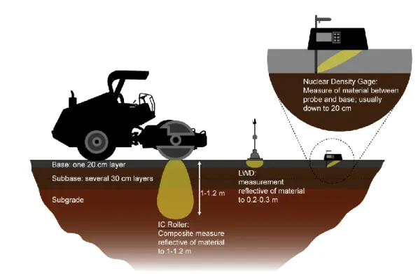
There are currently two commonly used potential definitions of the force-displacement roller MV k and ks, as used by different IC roller manufacturers. Both of these measures (Bomag stiffness and Case/Ammann stiffness) are determined from force-displacement loops, interpreted from the drum acceleration time history data, collected by IC rollers. These force-displacement loops are created by plotting the time-varying contact force, Fc, versus time-varying drum displacement, zd. Fc is calculated from the vertical response of the drum; see Figure 2.1(Mooney and Rinehart 2009). Equation 2.3 is derived from equilibrium where m0e0 is the eccentric mass moment of the eccentric vibratory masses on the roller; ω is the frequency of the rotating eccentric masses; ϕ is the eccentric force phase shift between the inertia force of the drum ( ̈ ) and the eccentric excitation force ( ); md and mf are the drum and frame masses,
respectively; g is the acceleration due to gravity; and ̈ and ̈ are the drum and frame accelerations, respectively (Anderegg and Kaufmann 2004; Mooney and Adam 2007; van Susante and Mooney 2008). The drum displacement, zd, is calculated by taking the double
9
integration of the drum acceleration data. Bomag soil stiffness (k in Figure 2.2) is calculated from the tangent to the force-displacement loop at locations of 80% and 20% of the difference between maximum and minimum contact force (Mooney et al. 2010). From this soil stiffness,
Evib may be determined from back calculations and the stiffness can be converted into a modulus using the relationship for a drum on an isotropic elastic half-space (Mooney and Adam 2007; Facas 2010). Ammann and Case soil stiffness (ks in Figure 2.2) is calculated from the gradient of the line passing through the point of zero dynamic displacement (i.e. at the displacement of the soil surface due to the static weight of the roller) to the point of maximum dynamic drum displacement (Anderegg and Kaufmann 2004; Mooney et al. 2010).
Figure 2.1 Free body diagram of forces acting on the vibratory roller (from Mooney and Rinehart 2009)
( ) ̈ (2.3)
2.2 Intelligent Compaction Specifications
Currently there are many states conducting demonstration projects and pilot programs using IC rollers, integrating them into earthwork projects (e.g. Peterson 2005; Camargo et al. 2006; Zambrano et al. 2006; Rahman et al. 2008; White et al. 2008; Liu et al. 2011). These programs are developing specifications for IC in the U.S. for use during QA/QC procedures (e.g.
10
MnDOT 2010; TxDOT 2008). Many of these specifications being developed are based on European specifications (Rinehart et al. 2012). There are two approaches used in the European IC specifications: (1) spot testing of roller identified weak areas; and (2) calibration of roller MVs to spot test measurements (Rinehart et al. 2012).
Figure 2.2 (a) force-displacement loop during contact mode; (b) force-displacement loop during partial loss of contact mode (from Mooney and Facas 2012)
In current QA/QC procedures spot testing is performed at random locations, and if the testing locations chosen pass the relative compaction requirement, then the whole area passes. With approach (1), roller MVs can be used to identify weak areas for the earthwork site and then these areas can be tested. This is stricter than testing at random locations and this approach was proven to be acceptable for use with IC (Rahman et al. 2007; Rinehart et al. 2012). Approach (2) of calibrating spot test measurements to roller MVs was proven to not be a useful approach to use with IC and needs further analysis. With this approach an MV target value is determined from calibrating the roller MV to spot test measurements. After calibration, the target MV is used to determine which areas pass and which areas fail the compaction requirement. This approach is not useful because it was found, after calibration, some areas would meet the spot
11
test density requirement and not meet the target MV, so the calibration techniques need to be improved for this approach (Rinehart et al. 2012).
Another approach that has been suggested is to use the mean MV to assess the general condition of the entire checked area. It has been suggested to use limits for minimum, maximum, and mean MVs as well as limits on the standard deviation. The proposed approach requires a standard deviation of less than 20%, related to the mean value, and less than a 5% increase in the mean roller MV between passes (Adam and Kopf 2004). This approach has also been proven to be an acceptable approach for use with IC but verification testing (i.e. spot testing) is still needed because it does not necessarily ensure the desired compaction level has been met (Adam and Kopf 2004; Facas et al. 2011).
2.3 Roller Measurement Depth
The roller MVs have been shown to be influenced by the underlying soil 1.0 – 1.2 m deep in vertically homogeneous conditions (Rinehart and Mooney 2009; Mooney and Facas 2012). This depth, in most cases, will consist of multiple lift layers. Earthwork construction involves combinations of subgrade, subbase, and base material lifts where the lift layers are commonly 15 – 30 cm thick, shown in Figure 2.3 (Mooney and Facas 2012). The roller MV is therefore a composite value not only of the top lift of soil but the underlying lifts 1.0 – 1.2 m deep. Typical spot testing techniques, such as nuclear density gauge and light weight deflectometer (LWD), only measure the soil density of the top lift 20 – 30 cm deep. Roller MVs are commonly used in correlation with spot test measurements, and the difference in measurement depth presents a problem in relating the two (Thompson and White 2007). Also all U.S. transportation agencies perform QA/QC on a per lift basis so, for IC to be most effective the soil properties of the top lift would need to be extracted (Mooney and Facas 2012).
12
Figure 2.3 Measurement depth of intelligent compaction rollers and spot tests (from Mooney and Facas 2012)
Each lift of the soil system has a specific purpose and the strength of each layer has an impact on the overall strength of the system (Burmister 1958). The subgrade soil is used to support the wheel loadings imposed by traffic on the soil system. The subbase and base lift materials help reinforce and distribute the load to protect the subgrade material, this helps distribute the stress and reduce the deformation on the subgrade layer (Burmister 1958). In order to assure the soil system has the required design strength properties, the strength of each
individual lift is important. With roller MVs being affected by soil 1.0 – 1.2 m deep less than half of the soil affecting the MV is from the top lift. This presents another problem when using MVs to determine the strength properties of the soil system. The effect of layered soils on MVs needs to be investigated further to better understand how lift thickness and underlying soil systems affect roller MVs.
13 2.4 Roller Modes of Operation
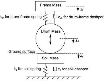
From previous analyses of vibratory roller behavior, there have been three common modes of operation identified and widely researched. These modes are contact, loss of contact, and chaotic motion or bifurcation. Contact mode is where the drum of the roller is always in contact with the soil. Loss of contact mode is where the drum will lose contact with the soil once per cycle of vibration. Chaotic motion or bifurcation is where the drum of the roller will “jump” or “bounce” off the soil and lose contact with the soil at periodic intervals. This chaotic motion is not useful for compaction because it can lead to loosening of the top layer of soil, and it can also be dangerous for the operator and roller because the roller loses its maneuverability (Anderegg and Kaufmann 2004). As the stiffness of the soil increases during compaction the operating mode goes from contact to loss of contact to chaotic motion. IC rollers can automatically adjust the operating parameters of the roller to stop chaotic motion when it starts to occur by reducing the operating frequency and/or reducing the excitation amplitude. Without the use of IC it is up to the roller operator to adjust the operating parameters.
There have been many analytical models developed to model these three well known modes of operation (e.g. Yoo and Selig 1979; Pietzsch and Poppy 1992; Anderegg and Kaufmann 2004; van Susante and Mooney 2008). These models use lumped parameter
techniques, modeling the vertical motion of the roller and the drum-soil interaction. A typical 3-degree-of-freedom (DOF) model is shown in Figure 2.4, where the frame, drum, and soil are modeled as separate degrees of freedom. Lumped parameter values of drum-frame stiffness (kdf), drum-frame damping (cdf), soil stiffness (ks), and soil damping (cs) are chosen to calculate the frame displacement (zf), drum displacement (zd), and soil displacement (zs). These lumped
14
only able to model homogeneous soil conditions and do not account for multiple lift material properties on layered soils.
Figure 2.4 3DOF lumped parameter model (from van Susante and Mooney 2008)
2.5 Dependence of Roller Measured Values
Roller MVs have been proven to be affected by soil conditions (e.g. moisture content, subsurface anomalies) and roller operating parameters (Rahman et al. 2007; Thompson and White 2007; and Mooney et al. 2010). Since soil conditions and roller operating parameters can vary, roller MVs need to be calibrated so they can be accurately interpreted. Calibrating the MVs will ensure an increase or decrease in the MV measurement is representative of the compacted state of the soil, and not a change in the soil conditions or operating parameters.
Moisture content and subsurface anomalies are two soil conditions that have been shown to affect roller MVs (Rahman et al. 2007; and Thompson and White 2007). As the moisture content of the soil increases, the roller MVs decrease. This relationship requires the roller MVs to be calibrated to the moisture content or for the consistency of the moisture content over the testing area to be monitored in order to assure the MVs are not being affected by the variability in moisture content. The subsurface conditions also affect roller MVs because of the
15
measurement depth of vibratory rollers. With the roller MVs representing composite values of the soil 1.0 – 1.2 m deep the subsurface conditions will affect the roller MV. There can be locations of soft or stiff soils in the subsurface affecting the roller MV. These subsurface conditions cannot be accounted for because the subsurface conditions are usually unknown but they can be used to explain anomalies in roller MV data.
Some roller operating parameters that have been shown to affect roller MVs are eccentric excitation amplitude, roller speed, and driving direction (Mooney et al. 2010). The eccentric excitation amplitude can be adjusted during compaction to achieve the best compaction results. The excitation amplitude varies depending on the roller manufacturer but in most cases there is the choice of high, medium, and low amplitudes. It was shown by Mooney et al. (2010) the roller MVs most commonly increase with an increase in eccentric excitation amplitude. At higher amplitudes, the roller exhibits a greater amount of loss of contact behavior resulting in larger MVs. Roller speeds can also be adjusted during compaction. Mooney et al. (2010) showed roller speed has a direct correlation with MVs. As the roller speed increases the MVs decrease. The decrease in roller MVs with increasing speed was attributed to the vibration energy being spread over more soil at higher speeds, correlating to a reduced degree of loss of contact (Mooney et al. 2010). Most compaction processes involve driving the roller in both the forward and reverse directions, so the effect of driving direction on roller MVs was investigated. There was a subtle decrease in roller MVs when driving in the reverse direction compared to the forward direction. The decrease in MVs was subtle when driving in the reverse direction but still needs to be taken into account when interpreting forward and reverse travel MV data.
With the dependence of roller MVs on moisture content, subsurface anomalies, eccentric excitation amplitude, driving speed, and driving direction, the roller MVs need to be calibrated to
16
assure they are accurately interpreted. The soil conditions and roller operating parameters can vary depending on the earthwork site location and the roller manufacturer, so the roller MVs need to calibrated for each specific location where the rollers are used. The calibration of the roller MVs to the soil conditions and roller operating parameters ensures the full potential of IC methods are accurately used.
2.6 Influence of Rocking Motion
After further investigation into the roller behavior, it was also determined there is rocking motion of the drum that can affect roller MVs (Facas et al. 2010). This rocking motion occurs when the left and right sides of the drum rotate around the CG of the drum. Soil stiffness
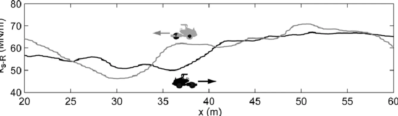
heterogeneity is the main cause for rocking, but rocking is also caused by asymmetry of the drum (Facas et al. 2010). This rocking mode was discovered by driving a Sakai IC roller over the same section of soil in opposite directions. It was discovered there were differences in the soil stiffness from instrumentation on the right side of the drum (ks-R) when driving in both directions, shown in Figure 2.5, where x is the northing location of the roller (Facas et al. 2010). The differences in
ks-R were caused by soil stiffness heterogeneity which caused the drum to rock.
17
This rocking behavior was modeled using a lumped parameter approach (Facas et al. 2010). The left and right sides of the drum were modeled as separate degrees of freedom allowing for differences in soil stiffness beneath the left and right sides of the drum to be taken into account, shown in Figure 2.6. This rocking model used springs to model the stiffness between the connections of the drum and frame and the stiffness of the soil and dashpots were used to model damping between the connections of the drum and frame and damping of the soil. The soil stiffness and damping parameters allowed for five evenly spaced springs and dashpots to be used along the length of the drum to take into account soil heterogeneity.
Figure 2.6 Lumped parameter rocking model (from Facas et al. 2010)
This rocking model was validated by independently instrumenting a Sakai SV510D IC roller with an EM accelerometer on both the left and right sides of the drum. By instrumenting both sides of the drum, the drum acceleration and MV can be calculated on both sides of the drum, and compared to the model. The model was first validated using a simplified 2DOF model. Data was collected while the frame of the roller was on jack stands and the drum was elevated off the ground. With the frame on the jack stands, it was fixed and did not move, and with the drum of the roller elevated off the ground, the only degrees of freedom were the left and right sides of the drum. Comparing the experimental data to the rocking model, the model was
18
able to accurately predict the drum acceleration and phase lag between the inertia force and eccentric excitation force on the jack stands. With the roller on the jack stands the acceleration on the right side of the drum was larger than the acceleration on left side of the drum, showing that rocking occurred even with the drum elevated off the ground. This proved that rocking not only occurs from soil stiffness heterogeneity but also from asymmetry of the drum (Facas et al. 2010).
Next the rocking model was validated from field data collected on transversely homogeneous and heterogeneous soil profiles. The soil profiles were determined from LWD testing (Facas et al. 2010). The stiffness profiles used for the rocking model matched the stiffness profiles from the LWD testing. The model was able to accurately predict the drum accelerations and the differences in left and right side drum accelerations for both the homogenous and heterogeneous soil profiles.
Manufacturers of IC rollers instrument one side of the roller to measure drum
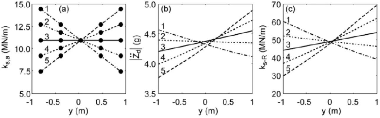
acceleration, and the location of this sensor can vary between manufacturers (Facas 2010). As shown by Facas (2010) the drum acceleration can vary on the left and right sides of the drum, indicating the location of the sensor can affect the MV. The effect of the sensor location was investigated with the rocking model developed by Facas et al. (2010). There were five sensor locations investigated, where the sensor location was measured as the distance from the drum CG (i.e. the drum CG was located at y = 0). There were also five different transverse soil profiles used where the soil stiffness, ks,a, is the soil stiffness at the five sensor locations investigated. Figure 2.7 shows the results from this study. These results show that rocking of the drum can affect transversely homogeneous soil, profile 3, because of the asymmetry of the drum and ks-R for transversely homogeneous soil can vary up to 23% depending on sensor location (Facas
19
2010). For the most transversely heterogeneous soil, profile 5, ks-R can vary up to 135%
depending on sensor location (Facas 2010). This shows the sensor position has a large effect on roller MVs and needs to be taken into account.
Figure 2.7 Influence of sensor position on drum acceleration and roller measured stiffness: (a) five soil stiffness profiles each with five discrete ks,a; (b) peak drum acceleration as a function of
sensor position; and (c) computed ks-R as a function of sensor location (from Facas 2010)
Since the MV can vary depending on sensor location and driving direction, the MV calculated for a specific area is not unique. During earthwork procedures the roller can be driven in both directions and in different patterns that are not always consistent. This requires the need for an MV that is directionally independent. Facas (2010) proposed using MVs at the CG of the drum. Typically the accelerometers used to measure drum acceleration are mounted toward the edge of the drum because the rotating eccentric masses prohibit sensors to be mounted at the drum CG (Facas 2010). Instead of mounting a sensor at the drum CG, the MV at the CG was derived using left and right side drum accelerations from the independently instrumented Sakai IC roller. The MVs calculated from EM sensors were referred to as EM MVs and the MVs derived at the CG were referred to as CG MVs, for this study (Facas 2010). The EM MV was calculated using the left side drum accelerometer.
The CG MV was proposed because there is no rotation at the drum CG and therefore there would not be any influence from rocking on the MV at this location. All drum
20
measurements are taken from the drum CG, where y = 0 at the drum CG. There was one EM accelerometer located on the left side of the drum at y = -0.853 m and one accelerometer located on the right side of the drum at y = 0.697 m. The acceleration (A) at any distance (d) along the drum can be calculated from the acceleration at the CG (Acg) and the angular acceleration (α) of the drum from Equation 2.4 (Facas 2010). Using the left and right side accelerometer locations at a distance d1 and d2 from the drum CG, respectively, Equation 2.4 can be solved for Acg and α,
given in Equations 2.5 and 2.6.
( ) (2.4)
( ) ( ) (2.5)
( ) ( ) (2.6)
Using Acg, the CG MV was calculated the same way the EM MV was calculated. The CG MV was then used to determine if it is directionally independent. From Figure 2.8 the CG MV is clearly less directionally dependent than the EM MV. The positive driving direction is from left to right and negative driving direction is from right to left in Figure 2.8. The CG MV is constant when driving in both the positive and negative directions where the EM MV varies when driving in the positive and negative directions. This shows the CG MV is directionally independent and is a better way to represent the MV.
The CG MV is an improvement upon the current techniques using EM MV, as it takes into account the dynamic behavior on both sides of the drum. The CG MV is independent of driving direction but it is still spatially dependent. When using IC during QA/QC the roller MVs are often compared between passes and if the roller is not driven over the same location for each
21
pass the soil heterogeneity can still affect the results. The CG MV is used to determine the MV at the CG of the drum, and if the CG of the drum is not driven over the same location, then the MV will be representing the soil properties at a different location. Since the validation of the CG MV was mostly conducted with lumped parameter modeling techniques, further investigation into this CG MV is still needed to better understand its effectiveness.
Figure 2.8 Directional dependence of EM MV and CG MV (from Facas 2010)
Since the soil heterogeneity can have such an impact on the roller MVs it would be useful to quantify the heterogeneity under the drum of the roller. This would allow the variation in soil conditions and the effects of drum rocking to be better understood. One method to quantify heterogeneity proposed by Facas (2010) is to take the difference in the roller MV calculated from the left and right sides of the drum. With accelerometers located on both sides of the drum, both a left and right side MV can be calculated, and the difference in the left and right side MV (ΔMV) could be calculated. This method was tested but it was proven to be an ineffective method because the ΔMV was dependent on driving direction (Facas 2010). When driving over the same area of soil in one direction and then turning around and driving in the opposite
22
drum. Since ΔMV varies depending on driving direction this is not a useful method for quantifying heterogeneity.
Another method proposed by Facas (2010) was to use the angular acceleration, α, to calculate a rotational stiffness, and use this rotational stiffness to quantify heterogeneity. This method was not investigated any further because the applied moment is needed to calculate the rotational stiffness and this was currently not possible (Facas 2010). This method of using a rotational stiffness to quantify heterogeneity can be investigated further to determine if a rational stiffness can be calculated, and used to quantify soil heterogeneity.
2.7 Research Potential
Since the discovery of the 1.0 – 1.2 m roller sensitivity depth, there have been very few experimental studies performed on how roller MVs are affected by layered soil systems (e.g. Adam 2007; Mooney and Rinehart 2009; Rinehart and Mooney 2009; Vennapusa et al. 2009; Rich 2010; White et al. 2011). Since most lifts’ are 15 – 30 cm thick, these lifts’ make up less than half of the composite roller MV of the underlying soil system. Therefore, it is not yet known how roller MVs are affected by varying lift thicknesses and different lift materials. Since all U.S. transportation agencies perform QA/QC on a per lift basis, it is important to know if roller MVs are capturing the compacted state of the top lift of material or if the roller is not sensitive to this top lift because of the roller measurement depth. This research will address these issues by performing a detailed analysis of how the roller MV ks is affected by various lift configurations, lift thicknesses, and lift materials.
Also, the discovery of the rocking motion of the drum has proven the roller MVs are dependent on sensor location, but there has been very little field data analyzed incorporating the influence of sensor location into the MV measurement. There was both left and right side drum
23
field data collected for the layered soil analysis performed in this study, providing information on how roller MVs can vary depending on sensor location. The left and right side drum field data will be analyzed to determine how to incorporate sensor location into the ks measurement,
building on what Facas et al. (2010) discovered with the CG MV being a better representation of the roller MV because no rocking occurs at the CG of the drum.
24 CHAPTER 3
ANALYSIS OF CENTER OF GRAVITY ROLLER DRUM VIBRATION AND RESULTANT SOIL STIFFNESS ON COMPACTED LAYERED EARTHWORK
Modified from a paper submitted June 2013 to the ASCE Journal of Geotechnical and
Geoenvironmental Engineering
Aaron Neff, S.M. ASCE1; Judith Wang, A.M. ASCE2; and Michael Mooney, M. ASCE3 Interest in intelligent compaction (IC) for earthwork procedures has steadily grown over the past decade, wit1h many states conducting demonstration projects and pilot programs (Petersen 2005; Camargo et al. 2006; Zambrano et al. 2006; Rahman et al. 2008; White et al. 2008; Mooney et al. 2010; Liu et al. 2011). By monitoring a vibratory roller’s vertical drum acceleration and the position of the rotating eccentric mass during the compaction process and after compaction during proof rolling, the underlying soil stiffness can be estimated in real time and continuously (Anderegg and Kaufman 2004; Sandstrom and Pettersson 2004; Brandl et al. 2005; Mooney and Adam 2007; Mooney and Rinehart 2007). This provides a significant improvement over conventional ‘spot’ testing and moves the pavement community towards the assessment of mechanistic parameters that are used in design, e.g., elastic modulus.
It has been previously shown that 12 – 15 ton smooth drum vibratory rollers provide a measure of composite soil stiffness reflecting the behavior to a depth of 1.0 – 1.2 m deep in vertically homogeneous conditions (Rinehart and Mooney 2009). Given that many earthwork situations include 15 – 30 cm thick lifts of different materials (base, subbase, subgrade), the
1
Graduate Research Assistant; Department of Civil and Environmental Engineering, Colorado School of Mines; 1500 Illinois Street, Golden, CO 80401; aneff@mines.edu
2
Assistant Professor; Department of Civil and Environmental Engineering, Colorado School of Mines; 1500 Illinois Street, Golden, CO 80401; judiwang@mines.edu
3
Professor; Department of Civil and Environmental Engineering, Colorado School of Mines; 1500 Illinois Street, Golden, CO 80401; mmooney@mines.edu
25
roller measured soil stiffness is often a composite value capturing the combined response of multiple lifts. Very few experimental studies have examined IC roller behavior on layered soil systems (e.g. Adam 2007; Mooney and Rinehart 2009; Rinehart and Mooney 2009; Vennapusa et al. 2009; Rich 2010; White et al. 2011). These studies have shown the roller measured soil stiffness increases when adding stiffer subbase and base lifts on top of softer subgrade lifts but further analysis of layered soil systems in needed to better understand the effect of varying lift thicknesses and lift configurations on the composite soil stiffness measure.
Additionally, IC roller manufacturers currently instrument only one side of the roller drum with accelerometer(s) for the calculation of an EM roller measured soil stiffness. This assumes that the EM soil stiffness is representative of the soil stiffness under the entire width of the drum. However, rocking motion of the drum, where the left and right sides of the drum rotate around the drum CG has been proven to affect EM soil stiffness (Facas et al. 2010). This rocking motion occurs due to drum asymmetry and soil heterogeneity, and influences EM soil stiffness significantly (Facas et al. 2010). Facas et al. (2010) showed that drum rocking can have a significant influence on the reported EM soil stiffness, with the left vs. right EM soil stiffness varying over 100% in some cases. This motivated Facas et al. (2010) to propose a roller measured soil stiffness at the CG of the drum. CG soil stiffness is calculated at the center of rotation; thus, variable sensor distances and drum rocking do not affect the resulting values (Facas et al. 2010). The CG soil stiffness was developed using lumped parameter modeling techniques; but has not yet been widely implemented in the analysis of full-scale IC field data.
Therefore, the objective of this paper is to present detailed experimental data from two full-scale layered earthwork systems, exploring the sensitivity of CG soil stiffness to lift materials and thicknesses. The data were collected from two layered earthwork sites in Florida
26
and North Carolina using a Sakai SV510D smooth drum vibratory roller instrumented with EM (left and right) accelerometers located at known distances from the CG. This study provides the first detailed analysis of experimental data from layered soil situations using CG soil stiffness, demonstrating the efficacy of this measure and its sensitivity to underlying layered soil
conditions for real-world IC procedures.
3.1 Field Data
Field data from two locations in Florida and North Carolina were collected and analyzed for the purposes of this study. The Florida site provides the bulk of the analyzed data and forms the basis for the observed trends in roller measured soil stiffness and roller behavior with respect to the underlying soil system. The data from the North Carolina site are used to verify the trends identified from the Florida site.
3.1.1 Florida Earthwork Site
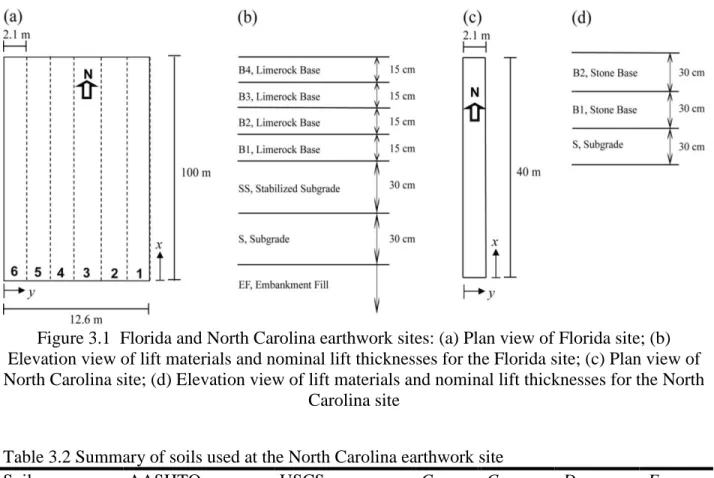
The layered soils at the Florida site are shown in Figure 3.1a and 3.1b. The lift soils include embankment fill (EF), subgrade (S), stabilized subgrade (SS), and limerock base lifts (B1, B2, B3, and B4). A summary of the Florida lift materials are shown in Table 3.1. The EF was the existing and previously compacted soil material onsite, with no one specific soil
classification recorded; however, it was visually classified to be a sand material similar to the S material. Each lift of soil material was 100 m long and six roller lanes wide, with each lane equaling the width of the roller drum (2.1 m). Each lift was compacted with the Sakai instrumented smooth drum vibratory roller and mapped upon completion of compaction. Mapping involves collecting vertical drum acceleration, eccentric mass position, and roller position data while driving the roller over each lane of the lifts after compaction was complete.
27
The mapping data on each of the lifts will be the data used for the analysis. The operating frequency of the roller for the EF, S, SS, and B1 lifts was 30 Hz, and the operating frequency of the roller for the B2, B3, and B4 lifts was 25 Hz. These frequencies were chosen by the on-site operators to accommodate on-site construction conditions.
Table 3.1 Summary of soils used at the Florida earthwork site
Soil AASHTO Classification USCS Classification Cu Cc D50 (mm) ELWD (MPa)
Embankment Fill N/A N/A N/A N/A N/A N/A
Subgrade A-3 SP: Poorly
graded sand with gravel 2.1 0.88 0.28 59 Stabilized Subgrade 23 cm of A-3 subgrade with 7 cm of stabilizing ash
N/A N/A N/A N/A 60
Limerock Base A-1-b GW: Well
graded gravel with sand
90 0.90 5.1 85
The lightweight deflectometer (LWD) modulus value (ELWD) in Table 1 is based on LWD spot testing analysis performed after compaction of each lift was complete. LWD testing
involves dropping a weight onto a circular plate and measuring the deformation of the soil surface due to the applied load. ELWD values are then calculated using circular plate on elastic half-space theory and may be used to represent relative stiffness properties of soil materials (e.g. Mooney and Miller 2009). The ELWD values in this study are used to provide information on the relative stiffness properties of the different lift materials in the stratified foundations (Mooney and Miller 2009).
3.1.2 North Carolina Earthwork Site
The layout of the lifts at the North Carolina site is shown in Figure 3.1c and 3.1d, consisting of only one lane 2.1 m wide and 40 m long. There were three lifts at the North
28
Carolina site including one subgrade (S) and two stone base lifts (B1 and B2). A summary of the North Carolina lift materials used are shown in Table 3.2. The mapping data for all lifts are used for the analysis of the North Carolina site. The operating frequency of the roller was 30 Hz on all three lifts.
Figure 3.1 Florida and North Carolina earthwork sites: (a) Plan view of Florida site; (b) Elevation view of lift materials and nominal lift thicknesses for the Florida site; (c) Plan view of North Carolina site; (d) Elevation view of lift materials and nominal lift thicknesses for the North
Carolina site
Table 3.2 Summary of soils used at the North Carolina earthwork site
Soil AASHTO Classification USCS Classification Cu Cc D50 (mm) ELWD (MPa)
Subgrade A-4 SW-SM: Well
graded sand with silt and gravel
53 1.9 1.2 45
Stone Base A-1-a GW-GM: Well
graded gravel with sand and silt
67 0.67 7.0 60
3.2 Roller Instrumentation and Center of Gravity Soil Stiffness
The Sakai SV510D smooth drum vibratory roller was outfitted with vertical
29
record the rotational position of the eccentric mass with time. The roller was also equipped with a differential Global Positioning System (GPS), allowing the easting position, northing position, and elevation of the roller to be determined with cm level accuracy. The northing and easting locations are denoted in this paper as x and y, respectively. The elevation data are used to
calculate individual lift thicknesses, h, by taking the difference in elevation between consecutive lifts.
Roller measured soil stiffness (ks) may be determined from force-displacement loops post-processed from recorded acceleration data (Figure 3.2). These force-displacement loops are generated by plotting the contact force (Fc) of the drum on the soil versus drum displacement (zd).
Figure 3.2 Force-displacement loops on the S lift at the North Carolina site showing roller measured soil stiffness, ks
Fc is calculated using Equation 3.1, where m0e0 is the eccentric mass moment of the eccentric vibratory masses on the roller; ω is the operating frequency of the rotating eccentric masses; ϕ is the phase lag between the eccentric excitation force and drum displacement; md and
mf are the drum and frame masses, respectively; g is the acceleration due to gravity; and ̈ is the measured drum acceleration (van Susante and Mooney 2008). zd is calculated from ̈ , where ̈
30
is integrated twice using the trapezoidal rule and numerical drift in the integration is accounted for by subtracting out the linear trend in the integrated data. ks is then calculated as the gradient of the line passing through the point of zero dynamic displacement (i.e., at the displacement of the soil surface due to the static weight of the roller) to the point of maximum dynamic drum displacement (Anderegg and Kaufmann 2004; Mooney et al., 2010).
( ) ̈ (3.1)
Currently all IC roller manufacturers only instrument one side of the roller drum for the calculation of ks, known as an EM soil stiffness. This EM soil stiffness is not unique for a given underlying soil, as it can vary significantly depending on the distance of the accelerometer from the drum CG due to rocking of the drum caused by drum asymmetry and/or soil heterogeneity (Facas et al. 2010). In the configuration examined in this study, the distance of the left
accelerometer to the drum CG was dL = -0.853 m, and the distance of the right accelerometer to
the drum CG was dR = 0.697 m (see Appendix A for illustration showing the distances dL and
dR). The difference in calculated EM soil stiffness values from the left and right sides of the drum is shown in Figure 3.3, for EF, lane 3 data collected at the Florida earthwork site.
31
To remove this dependence on rocking, Facas et al. (2010) proposed a CG soil stiffness (ks-CG). If a sensor could be located at the drum CG, there would be no effect of rocking at this location as the drum rotates around the CG (Facas et al. 2010). The location of the eccentric masses inside the drum of the roller do not allow for a sensor to be mounted at the drum CG, but the drum acceleration at the CG ( ̈ ) can be calculated using Equation 3.2, using the
measured left and right accelerations ( ̈ and ̈ , respectively) from accelerometers located at dL and dR (Facas 2010).
̈ ̈ ̈
(3.2)
̈ can then be used in conjunction with the aforementioned procedures, calculating Fc-CG, zd-CG , and ks-CG from ̈ . ks-CG removes the effects of rocking inherent in EM soil
stiffness, providing one, unambiguous composite soil stiffness measure for each x-y location for an underlying soil system. EM soil stiffness from the left or right sides of the drum give two measures of soil stiffness for one location; additionally, EM soil stiffness will be different when driving over a section of soil and then turning around and driving over the same section of soil in the opposite direction (Facas et al. 2010), showing an artificial directional dependence. Since roller measured soil stiffness values are usually compared from pass to pass and driving direction is not always consistent, it is important to have a soil stiffness measure that is directionally independent. It was shown by Facas et al. (2010) that, when driving the roller over the same section of soil in one direction and then turning around and driving over the same section of soil in the opposite direction, the EM soil stiffness varies significantly while ks-CG is relatively constant. ks-CG is therefore used in this study as the composite measure of underlying soil
32
stiffness to remove the aforementioned ambiguities associated with EM soil stiffness values (for supplemental rocking analysis see Appendix A).
3.3 Analysis of Florida Data
ks-CG measured at the Florida site will be compared for consecutive lifts to determine relationships between changes in ks-CG, lift thicknesses, and lift materials. There is a large amount of variability in ks-CG from lane to lane on all of the lifts. Figure 3.4 shows ks-CG across all lanes for the EF lift; the width of each of the lanes is 2.1 m but is plotted with a width of about 1 m such that the data in the different lanes are readily distinguishable. The lanes are 100 m long, but only the data from x = 35 – 75 m are shown; at the omitted ends of the lanes, the roller was turning around between passes and the data are not as readily useful.
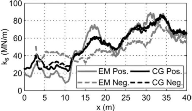
Figure 3.4 ks-CG for the EF lift
In the direction of roller travel (x direction) ks-CG varies considerably but smoothly because the interval between each measurement is 3-5 cm (see Facas and Mooney 2010).
Transverse to the direction of roller travel (y direction), the change in ks-CG is more abrupt due to natural soil heterogeneity coupled with a single measurement for a 2.1 m long drum. Due to the
33
large variability in ks-CG from lane to lane, only overlapping lanes where the roller was driven over the same x-y locations (within a 20 cm spatial tolerance) in each lane for the layered lifts can be accurately evaluated to determine the influences of h and lift material on ks-CG. To determine appropriately overlapping x-y locations for the layered lifts, the GPS data are
compared. An example of the determination of overlapping x-y locations is shown in Figure 3.5, where the travel path of the drum on the EF and S lifts and the corresponding overlapping location are shown. One section where the roller was driven over the same y location (within x cm tolerance), for consecutive lifts, will be presented for each lift (for complete analysis of all overlapping x-y sections for the Florida site see Appendix C).
Figure 3.5 Comparison of center of drum travel path for EF and S lifts; circled region indicates the area over which IC data is compared.
The first two lifts at the Florida site are the EF and S lifts. ks-CG are compared along similar x-y paths from x = 35 – 75 m in lane 1. Figure 3.6 shows the variation in lift thickness hs, compares the EF and S lift ks-CG values and provides the change in soil stiffness Δks-CG from the EF to the S lift as a percent. Figure 3.6 also presents contact force vs. drum CG displacement
34
response for x = 70 m as a way to illustrate changes in ks-CG and overall force-displacement response.
Figure 3.6 Comparison of EF and S lift from x = 35 – 75 m in lane 1: (a) S lift thickness, hs; (b) EF and S ks-CG; (c) percent change in ks-CG from EF to S; (d) force-displacement loops
From the EF lift to the S lift, ks-CG changes very little, with Δks-CG ranging less than ±10%. Δks-CG seems to trend with increasing hs; however, this is not a strong trend given the very low values of Δks-CG. The slight decrease in ks-CG from x = 41 – 58 m could be correlated to the compacted state of the S lift at this location and the variation in roller travel path from x = 49 – 59 m. There was no in-situ measurements recorded to verify compaction at this location but the varying roller travel path can be seen in Figure 3.5. Similar roller-measured soil stiffness is expected as the EF lift material and S lift material were judged on-site to be mostly
35
homogeneous, sandy materials. Hence, adding a compacted lift to a half-space of a similar soil should not influence ks-CG. Facas (2010) also showed there is a natural variability in ks-CG of up to 10%, and Δks-CG lies within this tolerance range, showing the change in soil stiffness from the EF to the S lift can be contributed to the variability in the roller measurement system. The similar behaviors of the EF and S lift force-displacement loops demonstrate the source of correlation in
ks-CG.
Figure 3.7 Comparison of S and SS lifts from x = 35 – 65 m in lane 2: (a) SS lift thickness, hss; (b) S and SS ks-CG; (c) percent change in ks-CG from S to SS; (d) force-displacement loops
The roller measured soil stiffness from the S and SS lifts are more discernible and are compared in Figure 3.7 along similar x-y paths from x = 35 – 65 m in lane 2 (driving paths not shown). The force-displacement loops for the S and SS lifts show an increase in SS contact force
36
with a slight increase in SS drum displacement. The combination of these trends produces a Δks-CG from the S lift to the SS lift ranging between 20 – 40%. This increase in ks-CG on the SS lift demonstrates that the roller is sensitive to the addition of 34 – 38 cm of compacted SS: the stabilized subgrade material is different enough from the unstabilized subgrade to affect ks-CG by a nontrivial amount. These data do not reveal a positive correlation between Δks-CG and hSS; rather, the results suggest a negative correlation. In this case, where the placed lift thickness (approaching 38 cm) is greater than that normally used (15 – 30 cm), it is plausible that the bottom of the SS lift was under compacted and thus softer. Unfortunately, we have no in-situ void ratio data (nearly impossible to measure) with depth to support this scenario.
Figure 3.8 Comparison of SS and B1 lifts from x = 55 – 75 m in lane 3: (a) B1 lift thickness, hB1; (b) SS and B1 ks-CG; (c) percent change in ks-CG from SS to B1; (d) force-displacement loops
37
IC roller data from the SS and B1 lifts are compared from x = 55 – 75 m in lane 3 (Figure 3.8). There is an increase in ks-CG from the SS lift to the B1 lift, with a Δks-CG of 18 – 26% over all sections analyzed. The B1 lift material is again different enough from the SS lift material that
ks-CG is sensitive to the change in material. There is no observed correlation between Δks-CG and
hB1 showing ks-CG is sensitive to the 9 – 14 cm thick B1 lift placed on top of the SS lift but not the small changes in hB1 (ΔhB1) of up to 5 cm. ks-CG on the SS and B1 lifts follow the same trends increasing and decreasing in tandem with respect to x, shown in Figure 3.8b. ks-CG on the B1 lift is influenced by the underlying SS lift and the addition of the B1 lift material but Δks-CG from the SS lift to the B1 lift is not affected by ΔhB1.
Figure 3.9 Comparison of B1 and B2 lifts from x = 35 – 51 m in lane 3: (a) B2 lift thickness, hB2; (b) B1 and B2 ks-CG; (c) percent change in ks-CG from B1 to B2; (d) force-displacement loops
38
B2 was compacted on top of B1 and mapped. The operating frequency on this B2 lift was decreased from 30 Hz, which was the operating frequency on the B1, SS, S, and EF lifts, to 25 Hz. This reduction in operating frequency was due to the fact that bifurcation (where the drum rebounds off of the soil at periodic intervals) was observed on the B2 lift at 30 Hz. Bifurcation is considered dangerous, as the roller loses its maneuverability; therefore, roller operators
typically adjust roller operating parameters on-site to avoid this behavior (Adam and Kopf 2004; Anderegg and Kaufmann 2004).
The B1 and B2 lifts are compared from x = 35 – 51 m in lane 3 (Figure 3.9). With the addition of the B2 lift, ks-CG increases by 8 – 16%. However, this increase is also related to the decrease in operating frequency from the B1 lift to the B2 lift (Mooney et al. 2010). Therefore, it is not immediately clear from the analysis of B1 to B2 alone how much of Δks-CG is due to increasing base lift thickness or to decreasing frequency between B1 and B2.
B3 was then added on top of the B2 lift and compacted and mapped at a constant
operating frequency of 25 Hz. The comparison of the B2 and B3 lifts from x = 55 – 75 m in lane 1 is shown in Figure 3.10. There is a Δks-CG of 7 – 23% from the B2 lift to the B3 lift. This increase in ks-CG is similar to the increase in ks-CG after adding the B2 lift, indicating that Δks-CG between B1 and B2 may have primarily been due to the increased thickness of the base material. There is also a correlation between ks-CG on the B2 and B3 lifts shown. Both the B2 and B3 lifts follow the same spatial trends along the section shown, increasing and decreasing in tandem with respect to x. There is no correlation between Δks-CG and hB3 confirming an observation from previous lifts, that ks-CG is sensitive to the addition of 9 – 20 cm thick base lifts but ks-CG is not sensitive to a Δh of up to 5 cm on the base lifts.
39
Figure 3.10 Comparison of B2 and B3 lifts from x = 55 – 75 m in lane 1: (a) B3 lift thickness,
hB3; (b) B2 and B3 ks-CG; (c) percent change in ks-CG from B2 to B3; (d) force-displacement loops
The section compared for the B3 and B4 lifts is from x = 55 – 75 m in lane 4 (Figure 3.11). The largest increase in ks-CG is with the addition of the B4 lift, with Δks-CG ranging between 20 – 60%. This large increase in ks-CG is seen from the force-displacement behavior: there is a large increase in contact force, correlating to a large increase in ks-CG. This large increase in ks-CG is not only due to the large ks-CG on the B4 lift but also a decrease in ks-CG on the B3 lift in this lane. Over most sections on the B3 lift, ks-CG ranges from 90 – 105 MN/m. In this lane, ks-CG stays around 80 MN/m except for at x = 66 – 67 m. This decrease in ks-CG in this lane on the B3 lift contributes to the large increase in ks-CG from the B3 lift to the B4 lift in this lane. From x =