Accuracy and precision of a technique to assess residual limb volume with a measuring-tape

(1)

School of Health Sciences, Jönköping University Department of Rehabilitation

Box 1026, SE-551 11 Jönköping

Accuracy and precision of a technique

to assess residual limb volume with a

measuring-tape

Gustav Jarl

Master’s Thesis, 10 credits, level 61-80 credits

Orthopaedic Engineering

Jönköping, June 2003

Tutor: Magnus Lilja, lecturer

(2)

Sammanfattning

Volymen på transtibiala stumpar kan förändras dramatiskt efter amputationen och försvåra protesförsörjningen. Skillnaderna mellan olika individer gör det svårt att ge generella rekommendationer om när patienten bör försörjas med definitiv protes. Detta skulle kunna lösas genom att mäta stumpvolymen på varje patient, men de flesta volymuppskattningsmetoder är för komplicerade för kliniskt bruk.

Syftet med studien var att utvärdera validitet och intra- och interpersonella reliabilitet för en metod att beräkna stumpvolymen från omkretsmått på stumpen. I metoden approximeras stumpen som ett antal avklippta koner och stumpänden som en del av ett klot.

Validiteten utvärderades teoretiskt i CAPOD på sex inscannade gipspositiv och manuellt på sex gipspositiv. Reliabiliteten utvärderades genom att jämföra mätningar gjorda av fyra personer på åtta stumpar. Mätningarna gjordes med en trälinjal och ett måttband av metall. Felen uppskattades med intraclass correlation coefficient (ICC), där 0,85 ansågs vara reliabelt, samt det kliniska kriteriet att ett volymfel på ±5% var acceptabelt (5% motsvarar en strumpa). I teorin visade sig metoden vara valid för alla gipspositiv men i de manuella mätningarna var den bara valid för fyra gipspositiv. ICC var 0,95-1,00 för intrapersonell reliabilitet men bara 0,76 för interpersonell reliabilitet. Både intra- och interpersonell reliabilitet var otillräcklig då kliniska kriterier användes. Felen orsakades av variationer i uppskattningarna av stumpändarnas längder och variationer mellan omkretsmåtten.

Metoden behöver utvecklas och är inte lämplig på spetsiga stumpändar. För att förbättra reliabiliteten rekommenderas att använda en lång linjal (ca 30 cm) med en ände som en vinkelhake för att mäta stumpändarnas längder. Att använda ett desinficerbart måttband i kombination med ett fjäderbelastat handtag kan förbättra reliabiliteten på omkretsmåtten.

(3)

Abstract

Transtibial stump volume can change dramatically postoperatively and jeopardise prosthetic fitting. Differences between individuals make it hard to give general recommendations of when to fit with a definitive prosthesis. Measuring the stump volume on every patient could solve this, but most methods for volume assessments are too complicated for clinical use. The aim of this study was to evaluate accuracy and intra- and interrater precision of a method to estimate stump volume from circumferential measurements. The method approximates the stump as a number of cut cones and the tip as a sphere segment.

Accuracy was evaluated theoretically on six scanned stump models in CAPOD software and manually on six stump models. Precision was evaluated by comparing measurements made by four CPOs on eight stumps. Measuring devices were a wooden rule and a metal circumference rule. The errors were estimated with intraclass correlation coefficient (ICC), where 0,85 was considered acceptable, and a clinical criterion that a volume error of ±5% was acceptable (5% corresponds to one stocking).

The method was accurate on all models in theory but accurate on only four models in reality. The ICC was 0,95-1,00 for intrarater precision but only 0,76 for interrater precision. Intra- and interrater precision was unsatisfying when using clinical criteria. Variations between estimated tip heights and circumferences were causing the errors.

The method needs to be developed and is not suitable for stumps with narrow ends. Using a longer rule (about 30 cm) with a set square end to assess tip heights is recommended to improve precision. Using a flexible measuring-tape (possible to disinfect) with a spring-loaded handle could improve precision of the circumferential measurements.

(4)

INTRODUCTION

A good fitting of the socket to the residual limb is an important factor to achieve a prosthesis that is functional to the patient (Johansson and Öberg 1998). Both volume and shape are factors influencing the degree of fit between the socket and the stump. Although shape may be a more valid measure of socket fitting, it is much harder to quantify than volume. It is also harder to construct clinical criteria for how stable the shape should be (how big the variations can be and at what sites) before fitting the patient with a definitive prosthesis. The focus of this thesis is the matching of volume between socket and stump.

To get the volume of the socket correct can be especially hard after the amputation when reduction of oedema, atrophy of muscles and weight changes can make the volume of the residual limb change dramatically. These problems make it easier to get the socket fit if one waits with the prosthetic fitting until the volume of the stump has stabilised. On the other hand the patient should be made mobile as soon as possible postoperatively to prevent deconditioning (Bowker et al. 1992). There is also an ambition to start gait training and rehabilitation as soon as possible postoperatively. This situation can be solved by the use of an inexpensive temporary prosthesis during a period postoperatively. (Fernie and Holliday 1982, Lilja and Öberg 1997) The crucial question is when the volume of the stump is stable enough for fitting with definitive prosthesis.

Different authors have investigated the changes in volume after amputation and some have come with recommendations about when the proper time is for fitting with definitive prosthesis (Fernie and Holliday 1982, Persson and Liedberg 1983, Golbranson et al. 1988, Lilja and Öberg 1997).

Fernie and Holliday (1982) measured the volume changes of 18 amputees (17 at transtibial level) with a water displacement technique. The measurement errors of the apparatus were evaluated in a previous study, but only for assessment of cross-sectional areas, not for volumes (Fernie et al. 1978). The results were presented as groups of patients with similar patterns of volume changes. No statistic method was used to separate the patients into different groups. The authors found volume changes not to have any single characteristic pattern and they therefore states that the time for prosthetic fitting cannot be predicted precisely by regular volume measurements postoperatively. The authors recommend fitting with definitive prosthesis after 150 days postoperatively.

Persson and Liedberg (1983) followed 93 transtibial stumps postoperatively. After 12 weeks the mean reduction in volume was 7,3% (standard deviation 10,6%) compared to two weeks postoperatively. The volume of the stump was approximated as a cut cone between circumferential measurements taken proximal and distal at the stump, respectively. The method for assessing volume is questionable but the results indicate big differences between individuals in volume changes postoperatively.

Golbranson et al. (1988) used a water displacement technique to estimate postoperatively volume changes of transtibial amputees. 36 individuals were divided into three groups receiving different treatments to stabilise limb volume. The first group was treated with elastic bandage, the second group had a plaster cast attached to a pylon and a SACH foot (elastic bandage when not ambulating), and the third group had a laminated socket with a

(7)

pylon and a SACH foot. The first group showed no significant volume changes over time, but the both latter groups showed significant reductions of volume over time. The correlation coefficients between volume and time were very low, between 0,08 and 0,30 for the different groups, indicating big variations between individuals. Like Fernie and Holliday (1982) the authors found volume stabilisation to be a highly individualistic process. Still, Golbranson et al. (1988) recommend that circumferences are measured postoperatively as a guide for permanent prosthetic fitting. This is almost completely the opposite of the statement by Fernie and Holliday (1982), that the proper time for definitive fitting with prosthesis cannot be predicted by postoperatively volume measurements.

Lilja and Öberg (1997) examined 11 transtibial amputees during 160 days postoperatively. The volume determinations were made with the CAPOD system which measurement errors have been evaluated in an earlier study (Lilja and Öberg 1995). The postoperative treatment consisted of fitting with temporary prosthesis and rehabilitation with physical training, gait re-education, prosthesis training, and occupational therapy. An elastic bandage was used after the surgical dressing had been removed. The authors found all patients to be ready for definitive prosthesis after 120 days, when using a criterion that one stocking is acceptable to wear in the socket. (When the authors used a two stockings criterion, the recommendation was to fit with prosthesis after 100 days) There were big variations between the individuals in the study, the first patient being ready for definitive prosthesis after 80 days and the last after 120 days.

Different postoperative treatments were used in the studies, and the treatments were not always described in detail. Golbranson et al. (1988) evaluated three different methods of stabilising limb volume: an elastic bandage, a plaster cast with a pylon and a SACH foot, and a laminated socket with a pylon and a SACH foot. In the study by Lilja and Öberg (1997) an elastic bandage was used after the surgical dressing had been removed and the postoperative treatment consisted of fitting with temporary prosthesis and physical rehabilitation. Persson and Liedberg (1983) do not report more than that the patients were kept in plaster of Paris during the first two weeks postoperatively and that the stitches were removed at three weeks. Fernie and Holliday (1982) do not describe the postoperative treatment at all. There are different philosophies of the postoperative treatment, concerning the dressing of the stump (rigid, semirigid, elastic, or more recently silicon liner), when to ambulate the patient, et cetera. The ideal would be to evaluate each postoperative method and compare the results to each other. Maybe are the volume changes different for different treatments, and maybe could the individual differences be reduced by some methods. The lack of homogeneity of treatments in the studies above questions the possibility of summing up the results from the different studies. On the other hand, although different treatments were used, the results all had one characteristic in common: the big variations between different individuals.

Both Fernie and Holliday (1982) and Lilja and Öberg (1997) give recommendations of when to fit with definitive prosthesis. The problem with general recommendations is that individual differences make the recommendations more or less accurate when applied on the individual. All the quoted studies show big differences in volume changes between different patients (Fernie and Holliday 1982, Persson and Liedberg 1983, Golbranson et al. 1988, Lilja and Öberg 1997). If these kinds of recommendations are accepted in clinical practice there is a risk that some patients get their definitive prostheses too early, which results in a need for a new socket after a short time. There is also a risk that other patients get their prostheses too late, and therefore get a worse rehabilitation than had been possible.

(8)

Another way to address the problem, instead of trying to find the one best time for prosthetic fitting, would be to develop a method to assess limb volume that could be used on every single patient. This would make it possible to make the decision of when to fit with a definitive prosthesis based on the patients own individual volume changes. Measurements could be recorded regularly after the amputation and be compared to the patient’s previous volumes and to shrinking patterns from scientific studies. Based on this, the proper time for fitting with definitive prosthesis could be selected. For example, if the volume immediately after the amputation is assumed to be 100%, a criterion could be to fit the patient with a definitive prosthesis when the volume change is less than ±5% in three weeks.

Yet most methods for volume determinations used in scientific settings are by different reasons not suitable for routinely clinical use. Water displacement technique (Fernie and Holliday 1982) can be too complicated to use as a clinical routine. Spiral X-ray computed tomography (Smith et al. 1995) and CAD/CAM systems (Lilja and Öberg 1995, Johansson and Öberg 1998) have also been used, but these systems require expensive equipment.

A proper method for clinical volume assessments would have to be simple to use, inexpensive, not very time consuming, and have an acceptable accuracy and precision. It is also an advantage if the method does not require much effort from the patient while most people amputated in the western world are elderly and can be in a poor physical condition. A simple method to assess transfemoral residual limb volume with a measuring-tape was described by Krouskop et al. (1979). Circumferences were measured at regular intervals and the stump volume was approximated as a number of cut cones between the measurement sites. The tip of the stump was approximated as a segment of a sphere. The method has never, what it comes to the author’s knowledge, been evaluated on transtibial stumps when it comes to errors of measurement.

(9)

THEORY

No matter if volume or some other characteristic is measured, a basic understanding of measurements and errors of measurements is essential in scientific work.

Measurements

A measurement can be defined as a way to procure symbols (often numbers) that represent characteristics of an object, an event, or a condition, where the symbols’ relations to each other are the same as the relations between the objects/events/conditions they are representing (Ackoff 1972).

Classification of measurements

In metrology measurements are traditionally classified into direct, indirect, and combined measurements. The combined measurements have more recently been divided into strictly combined and simultaneous measurements. (Rabinovich 1995)

Direct measurements are made by measuring an object with an instrument and reading the results direct on the instrument. Measuring circumferences of limbs with a measuring-tape is an example of direct measuring. The indirect measurements are based on knowledge of the relations between the quantity in interest and other quantities. The other quantities are measured and the wanted quantity is calculated from the results of the measurements. For example can mass and volume be measured to calculate the density of an object, while the ratio of mass and volume is the definition of density. (Rabinovich 1995) Although direct measurements are very common in ortopaedic workshops indirect measurements are probably never performed, at least not manually. CAD/CAM systems may use indirect measurements when calculating volumes of stumps from the scanned coordinates and the approximated shape.

Strictly combined and simultaneous measurements are closely related. In both cases several quantities are simultaneously measured (usually direct) and the values are put into a equation system that has to be solved. For strictly combined measurements, the measured quantities are of the same type. The equation system the results are put into is based on the relationship between arbitrary objects with the same measurable quantity. Assume that the mass of an object is known. The mass of several different objects can then be found by comparing different combinations of objects, and constructing equations from the results. For the simultaneous measurements, on the other hand, the measured quantities are of different kinds and the equations reflect relationships between the quantities in the nature. (Rabinovich 1995) Assume that the relationship between pressure and temperature of a gas is studied. The coefficient describing the relationship can be found by measuring the pressure by different temperatures and solving the equation system formed by the results. Strictly combined and simultaneously measurements are probably never performed in orthopaedic workshops. The strictly combined measurements can be viewed as a generalisation of the direct measurements and the simultaneous measurements as a generalisation of the indirect measurements. This means that, when it comes to the measurements physical significance, they can only be classified into direct and indirect measurements. Still, when the processing

(10)

of the data after the measuring is in focus, it is practical to distinguish between (a) direct, (b) indirect, and (c) simultaneous and combined measurements. (Rabinovich 1995)

Ackoff (1972) classifies measurements in an alternative way and take example of four types of measurements: numbering, counting, ranking, and measuring in a “restricted” sense. When

numbering, symbols (letters, numbers, et cetera) are put on objects or events and the symbols

are used as identification of the objects/events in the further processing of the data. No arithmetic operations can be performed with the symbols. When counting a number of positive values are put on elements in a class. For example can money of different denomination be counted: 20+0,5+10 = 30,5. The numbers resulting from the counting can be used in all kinds of arithmetic operations. The elements of interest can also be ranked, which means that the elements are put in a specific order depending on a specific relationship between the elements. Although numbers can be used to describe an element’s rank, no arithmetic operations can be performed with the numbers. Finally, there is also a measurement

in a restricted sense. These measurements are made with a constant measuring unit. (Ackoff

1972)

Scales of measurement

Depending on the characteristics of the measuring operations used a specific type of measuring scale can be chosen. When elements are numbered a nominal scale is used and when elements are ranked an ordinal scale is used. When measuring in a restricted sense, either an interval or a ratio scale is used. These four scales are the main types of measuring scales, but other types of scales can be obtained by combining the main scales (Ackoff 1972). All four scales have specific characteristics, which influence both the arithmetic and statistical operation possible to use on the material:

1. A nominal scale categorizes elements or groups of elements in different classes where all members in a class have some specific characteristic in common. It is useful to construct the classes so there is a class for every variation of the characteristic wished to classify and so the classes exclude each other, that is, so every element belongs to one class only. There is no specific order or ranking between the classes. (Ackoff 1972) As an example can patients be classified depending on their diagnoses and transtibial stumps depending on their shape (cylindrical, conical, or bulbous).

2. An ordinal scale ranks the elements in an order, so it is possible to state that a variable value is bigger (better, longer, et cetera) or smaller (worse, shorter, et cetera) than another value. The scale does not quantify the differences between the elements (Körner et al.1998). An example of ordinal scale is the sport medals; gold, silver, and bronze. When medical treatments are evaluated orally an ordinal scale is often (unconsciously) used. The patient is asked if he/she experience his/her condition as good/bad, improved/deteriorated, et cetera. Temperatures of limbs can also be ranked as warm, normal, or cold.

3. On an interval scale the elements are ordered and the distances between the elements are known. Usually the distances are the same between all scale steps, that is, the scale is linear, but the scale can also be logarithmic. There is no “natural zero” on the scale, which limits the mathematical operations possible to use. It is possible to calculate sums and differences, but not products and quotes. It is not possible to state that, for example, 20° Celsius is twice as warm as 10°, while the position of the point zero is arbitrary decided. Still, the most arithmetic operations can be performed with the differences between the values. (Ackoff

(11)

1972, Körner et al. 1998) To the author’s knowledge, the interval scale is not used in orthopaedic workshops.

4. On the last scale, the ratio scale, the elements are ranked, the distances between them are known, and there is an absolute zero on the scale. It is possible to calculate sums, differences, quotients, and products (Körner et al. 1998). An example of a ratio scale is the Kelvin scale, where the zero point is the absolute zero for temperature. 20° Kelvin is then really twice as warm as 10°. Volumes, lengths, and circumferences of limbs and ranges of motion of joints are measured on a ratio scale.

Obviously, the latter scales give more information about the measured variables than the former scales. When using the latter scales more types of statistical operations are also possible to use on the material (Ackoff 1972). The focus in this thesis is the measurements in restricted sense, either used on an interval or on a ratio scale.

Errors of measurement

Errors are present in almost all kinds of measurements, no matter what kind of measurement that is performed and what kind of scale that is used. Error of measurement can be defined as a deviation of the result from the true value. If µ is the true value of the quantity and x is the result of a measurement of µ, the absolute measurement error ζ is calculated as:

ζ = x-µ

Measurement errors can also be expressed in relative form as a fraction of the true value: ε = (x-µ) / µ

If the errors are very small, they are usually expressed as fractions of the measured value x. (Rabinovich 1995)

Errors of measurement are usually divided into systematic and random errors, each of them having specific characteristics and influences on the result. There are also errors that cannot be classified into these two main categories: the observer may read the result incorrectly, the observer may slip with the pen when notating the result, there may be error due to the rounding off of the numbers, et cetera. These kinds of errors also influence the final result but will not be treated in this thesis.

The infinite experiment and systematic and random errors

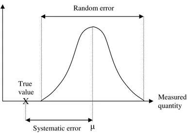
When a specific measurement is repeated under the same conditions the distribution of the results changes much at first, when the number of measurements is small. When the number of measurements increases the changes in the distribution become smaller. There is an assumption that if the measurement could be repeated an infinitive number of times the distribution would settle down to a specific shape, called the limiting frequency distribution curve or the parent distribution, Figure 1. If the curve is symmetric the mean, mode, and median are the same value and this value is usually chosen to be the “true” value of the experiment µ. If the curve is asymmetric it is a matter of convention which value is chosen, but most frequently the mean is used. (Boas 1983, Barford 1985)

(12)

The true value of the experiment µ is not necessarily the true value in reality; there may be a systematic error (also referred to as bias). If the systematic error is constant, it is the difference between the mean µ and the true value, Figure 1. The systematic error is not always constant; it may also vary periodically or according to some mathematical function and must then be evaluated in other ways. If the systematic error is very small or has been corrected for, µ can be assumed to be the true value. Accuracy (also referred to as validity) is the positive contrast to systematic error, where a high accuracy reflects a small systematic error. Accuracy can be described as a measure of to what extent a method measures what it is intended to measure (Dawson and Trapp 2001). Although the true value should ideally be used as a reference when evaluating accuracy, it is usually unknown. The result of the measurements is then compared to a reference technique known to be accurate, a “gold standard” (Hulley and Cummings 1988).

Still if µ is close the true value; there is a discrepancy between the individual measurements and µ. This discrepancy is called the random error and reflects the uncertainty of the result. Precision (also referred to as reliability) is the positive contrast to random error, where a high precision reflects a small random error. Repeating the measurements several times and using a statistical method to estimate the spread of the measurements estimates the precision. Usually the root mean square deviation σ, also called the standard deviation (SD), is used to estimate precision. The coefficient of variation (CV) is a “normalized” standard deviation, which is calculated by dividing the SD by the mean (Hulley and Cummings 1988). The range of the measurements can also be used (xmax-xmin) to estimate precision (Råde and Westergren 1995).

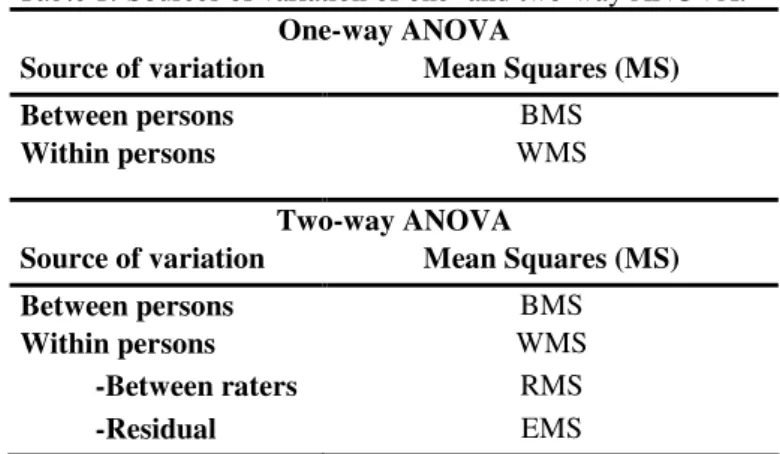
Intraclass correlation coefficients (ICCs) can also be used as estimates of precision (Shrout and Fleiss 1979). The ICC can be defined as the correlation between different measurements of the same object and describes the relative homogeneity of measurements within a “class”. There are three main forms of ICCs and they are all calculated with numbers obtained from an analysis of variance (ANOVA). Assume that a number of raters k measure a number of

Figure 1. Schematic illustration of parent distribution and systematic and random errors.

True value X Measured _quantity Systematic error Relative frequency of measurements Random error µ

(13)

randomly selected persons n. Assume further that the unit for the analysis is the individual measurements, that is, not means of several measurements.

The first form, ICC(1,1), is used when each person/object is measured by a different set of k raters. The raters are randomly selected from a larger population of raters. ICC(1,1) is calculated as:

where the components are obtained from a one-way ANOVA, Table 1.

The second form, ICC(2,1), is used when each rater makes measurements on each person/object. The raters are randomly selected from a population of raters. ICC(2,1) is calculated as:

where RMS is the mean square raters (variation within persons but between raters) and EMS is the residual mean square = total MS-BMS-RMS. All components are obtained from a two-way ANOVA, Table 1.

The third form, ICC(3,1), is also used when each person/object is measured by each rater, but when the raters in the study are the only raters of interest. The results of the study are then not possible to generalize to other raters than those participating in the study. ICC(3,1) is calculated as:

where the components in the equation are obtained from a two-way ANOVA, Table 1. (Shrout and Fleiss 1979, Laschinger 1992)

There are two ways to define agreement in the analysis. According to the first definition, consistency, measurements are in perfect agreement if they are equal or can be additively transformed to equality. According to the other definition, absolute agreement, values are in Table 1. Sources of variation of one- and two-way ANOVA.

One-way ANOVA

Source of variation Mean Squares (MS)

Between persons BMS

Within persons WMS

Two-way ANOVA

Source of variation Mean Squares (MS)

Between persons BMS Within persons WMS -Between raters RMS -Residual EMS ICC(1,1) = (BMS-WMS) . BMS + (k-1)*WMS ICC(2,1) = (BMS-EMS) , BMS + (k-1)*EMS + k*(RMS-EMS)/n ICC(3,1) = (BMS-EMS) , BMS + (k-1)*EMS

(14)

perfect agreement only if they are equal. For example are the paired numbers (2,4), (4,6), and (6,8) in perfect agreement using the consistency definition but not when using an absolute agreement definition. Additive transformation is performed by subtracting the mean of each rater from all individual measurements (the three paired numbers will then all take the form (-1,1)). ICC(1,1) and ICC(2,1) are measures of absolute agreement while ICC(3,1) is a measure of consistency. For a perfect agreement between the measurements the ICC will take a value of 1,00. There is no absolute lower limit for the ICC; it depends on the number of raters and is calculated as -1/(k-1). (Laschinger 1992, McGraw and Wong 1996)

The ICCs can also be calculated with the means of more than one rater’s measurements as the unit of analysis, instead of the single measurements. This approach usually makes the ICC higher, but the results cannot be generalized to individual raters, which is usually the purpose of the study. There have also been proposed other versions of ICCs than those presented here, but they will not be treated in this thesis. (McGraw and Wong 1996)

The previous discussion about errors of measurement is based on the concept of the infinite measurement. In reality the number of measurements is finite, and the true mean and standard deviation of the parent distribution can therefore not be precisely estimated. The measurements made can be viewed as a sample from the parent distribution, Figure 2. The mean of the parent distribution µ is then estimated by the mean of the measurements in the sample Xn: n x n ) x x (x X 1 2 n i n= + +…+ = ∑

where n is the number of measurements in the sample. The standard deviation of the parent distribution σ is correspondingly estimated by the standard deviation of the measurements in the sample s: 1 -n ) X -(x s 2 n i ∑ =

(Boas 1983, Barford 1985, Bevington and Robinson 1992)

Relative frequency of measurements

. Parent and sample distribution curves.

Measured quantity

(15)

In the same way as an infinitive number of single measurements can be imagined, an

infinitive number of sets of measurements can be imagined, each set giving a mean value X.

The standard deviation of a single measurement σ describes the spread of x values around µ

and how close to µ a single measurement is likely to be. Correspondingly, the standard

deviation in the mean σm (also referred to as the standard error) describes the spread of mean

values X around µ. It also shows how close to µ X is likely to be. The exact value of σm is not

known, but it can be estimated by the adjusted standard error sm, using the formula:

n s sm=

Where s is the standard deviation of the sample and n is the number of measurements in the

sample. sm is thus dependent of both the standard deviation of the single measurements and

the number of measurements made. The narrower the parent distribution f(x) is and the more measurements made, the closer to the true value X is likely to be. The result of a measurement can then be presented as the mean ± the adjusted standard error:

X±sm

When the number of observations increases in a sample, the sample distribution approaches

the parent distribution, Figure 2. The mean X approaches the true value µ and the standard

deviation of the individual measurements s, approaches the population standard deviation σ.

The standard deviation in the mean sm, on the other hand, approaches zero as the number of

measurements increases. (Boas 1983, Barford 1985)

The probability of an individual measurement x, or a mean X, to be at a given distance from µ

can be estimated with the help of the normal distribution. If the parent population f(x) is normally distributed and the sample is big enough (about 30) the sample distribution is approximately normally distributed. The probability of a single measurement to be within ±1 SD of the mean is then 68,3%, within ±2 SD 95,4%, and within ±3 SD 99,7%. (Gellert et al.

1989) The probability of a mean value X to be within ±1 SD of the true value µ is also 68,3%,

within ±2 SD 95,4%, and within ±3 SD 99,7%. The difference is that the latter probabilities are true for all functions g(X), no matter what the distribution is of the parent distribution f(x), if the sample is big enough. If f(x) is normally distributed the function g(X) is also normally distributed. If f(x) is not normally distributed, g(X) is approximately normally distributed if the number of measurements in the samples is large enough (about 30), according to the central limit theorem. (Boas 1983, Eason et al. 1992)

Propagation of error

The errors of the measurements have different influence on the final result depending on what operations that are performed on the results of the measurements. The measurements can in this context be divided into three groups depending on the processing of the data: (a) direct, (b) indirect, and (c) simultaneous and combined measurements (Rabinovich 1995).

Direct measurements

When performing direct measurements no further calculations are made on the material and the errors will therefore not be different in the final result than in the measurement itself. Still,

(16)

if the rater is not aware of the error of the measurements the person may misunderstand the result to be the “true” value.

Indirect measurements

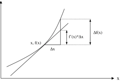
Indirect measurements are distinguished by that the measured quantities are not the quantities wanted in the final result. The results from the measurements are used in further calculations and the errors from the measurements will therefore propagate in the calculations. Assume that f(x) is a function of x and ∆x is the absolute error of x. The first, linear term in Taylor’s series is then usually accurate enough to evaluate the effect of ∆x on f(x), if ∆x is small enough or the higher derivates of f(x) are small enough. The error in f(x) can then be approximated by the equation for propagation of error:

∆f(x) = f’(x)*∆x [1]

Where f’(x) is the first derivative of f(x) evaluated in the point x, f(x), Figure 3. The true value of x is usually unknown, but an approximate value is usually sufficient and can be found experimentally. This equation is not exact, except when f(x) is a linear function of x: f(x) = a + bx

The higher derivatives in the Taylor’s series, f’’(x), f’’’(x), et cetera, are then zero and equation [1] reduces to

∆f(x) = b*∆x

which is exact for an error ∆x of any magnitude, not only for small errors.

Taylor’s series can also be used to estimate errors when a function includes several variables. Assume that f(x,y,z) is a function of the variables x, y, and z and ∆x, ∆y, and ∆z are the absolute errors of the variables, respectively. The effect of the errors on f(x,y,z) can then be approximated by an extension of equation [1]:

∆f(x,y,z) = Fx*∆x + Fy*∆y + Fz*∆z [2]

Where Fx = δf/δx, Fy = δf/δy, and Fz = δf/δz. Fx, Fy, and Fz are evaluated in the point (x,y,z) or

a point close, found experimentally. This equation can correspondingly to equation [1] be used if ∆x, ∆y, and ∆z are small enough or the higher derivatives (F’x, F’y ,F’z, F’’x, F’’y ,F’’z,

et cetera) are small enough. The only exception is when the function is linear, the equation is then exact for errors of any magnitude.

The formulas above are based on the assumption that the function can be approximated as a linear function, Figure 3. If the function is strongly non-linear or the errors of the variables are big, or rather when this is the case simultaneously, this approximation is not appropriate. Adding terms of higher order in the Taylor’s series to the equation can solve this. (Arnér 2002)

(17)

It is also possible to estimate the standard deviation of a function from the standard deviations of the measured variables. Assuming that the errors in the variables x, y, and z, are uncorrelated, the standard deviation of the function f(x,y,z) can be calculated with the formula: 2 2 2 + + = (F *σ) (F *σ) (F *σ) σf(x,y,z) x x y y z z [3]

where σx, σy, and σz are the standard deviations of x, y, and z, respectively. Equations [2] and

[3] can be used on functions with more than three variables, simply by adding more terms to the equations. Equation [2] can be summarized as:

∑       ∆ ∗ ∂ ∂ = ∆ x x x xn xi i 3 2 1 x f ) ,... , , ( f

Equation [3] can correspondingly be written in the shorter form:

2 i i f *σ x f 2 σ       ∂ ∂ ∑ =

(Bevington and Robinson 1992, Deming 1943, Gellert et al. 1989)

In reality, if the standard deviations of the measured quantities and the formula f(x) are known, the approximation formulas above are not necessary to use. The exact values of f(x) can then be calculated for each measured value and the standard deviation of f(x) can be calculated exactly without using any approximation. Earlier the approximation formulas were useful when the function f(x) was complicated, but after the introduction of computers this is not a problem anymore. Still, there is a use of these approximations when the function f(x) is unknown and is to be estimated by simple linear regression analysis. (Arnér 2002)

It is the belief of the author that indirect measurements are not a well-known area to most certified prosthetists and orthotists (CPOs). To estimate the error of the result demands both that the error of the measurements is known and that the propagation of the error is correctly

∆x f’(x)*∆x x f(x) ∆f(x) x, f(x)

(18)

calculated. The alternative way, to calculate the errors from the final result, is more exact and less complicated, and is therefore recommended.

Simultaneous and combined measurements

When performing simultaneous and combined measurements the results are substituted into a equation system that has to be solved. Usually the number of equations n is higher than the number of unknown variables m in the equation system. Because of the errors of measurement the unknown variables cannot be decided so all equations in the system are satisfied simultaneously. The conventional way is then to use the method of least square when choosing a solution of the system. (If n = m, the equation system can only be solved in one way, but there will still be errors in the result) Assume that the equation system has the form: Ax1 + By1 + Cz1 - l1 = 0 Ax2 + By2 + Cz2 - l2 = 0 . . . Axn + Byn + Czn - ln = 0

Or written more compactly as:

Axi + Byi + Czi - li = 0 [4]

where n is the number of conditional equations, i = 1,…, n, and n>3. A, B, and C are the unknown variables whished to estimate and xi, yi, zi, and li are the results of the ith serie of

measurements. When the estimations of the unknowns, a, b, and c, are substituted into

equation [4] there will be a residual vi because the estimations are not exact:

axi + byi + czi - li = vi [5]

The values of a, b, and c will then be chosen so the sum of the squared residuals gives a minimal value:

Q = Σvi2 = minimum

If the condition above is to be satisfied it is necessary that

0 c Q b Q a Q = ∂ ∂ = ∂ ∂ = ∂ ∂ [6]

If equation [5] is derived according to the three derivatives in [6] a system of equations is obtained. Using Gauss’ notation:

Σxi2 = [xx]

the equation system will take the form: [xx]a + [xy]b + [xz]c = [xl]

[xy]a + [yy]b + [yz]c = [yl] [7]

[xz]a + [yz]b + [zz]c = [zl]

(19)

The solution of a, b, and c, is calculated as: a = Dx / D

b = Dy / D

c = Dz / D

where the determinant D is:

[xx] [xy] [xz]

D = [xy] [yy] [yz] [xz] [zy] [zz]

and the determinants Dx, Dy, and Dz are found by replacing the first, second, and third

columns, respectively, in D with the right hand values of equation system [7]. For example,

Dx will take the form:

[xl] [xy] [xz]

Dx = [yl] [yy] [yz]

[zl] [zy] [zz] (Rabinovich 1995)

All determinants are calculated according to the standard equation: a11 a12 a13

a21 a22 a23 = a11a22a33 + a12a23a31 + a13a21a32 - a11a23a32 - a12a21a33 - a13a22a31

a31 a32 a33

(Råde and Westergren 1995)

The variance of the conditional equations can be found with the equation:

m -n v S 2 i 2 ∑ =

Where n is the number of conditional equations in the system and m is the number of unknowns (in this case three). The variances of the estimated values a, b, and c are calculated as: S * D D (a) S2 11 2 = *S D D (b) S2 22 2 = *S D D (c) S2 33 2 =

where D11, D22, and D33 are the algebraic complements of the elements [xx], [yy], and [zz] of

the determinant D, respectively. They are found by eliminating the row and column in D that the element belongs to. (Rabinovich 1995)

The formulas above are based on the assumption that the conditional equations in the equation system have equal variances, and they cannot be used when the variances are unequal. This can be the case when the different equations in the systems are reflecting measurements made under different conditions, but this will not be treated in this thesis. The method of least

(20)

squares is further only possible to use when the conditional equations are linear. When the equations are non-linear they have to be transformed to a linear form, but this is also beyond the scope of this thesis. (Rabinovich 1995)

In ortopaedic workshops simultaneous and combined measurements are never performed (if not inside some CAD/CAM system) and the propagation of these errors are therefore not relevant to the clinically active CPO.

Determination and correction of errors

It is important to be aware of measurement errors, while they are present in all kind of measurements and influence the results obtained. Errors of measurement are hard to eliminate, the challenge is rater to reduce the errors within acceptable limits. Systematic errors can be corrected for, if the magnitude of the error is known. Still, the exact magnitude of the systematic error is not known and the correction will therefore not be completely correct. This means that there will always be a small rest of systematic error, even after a correction has been introduced (Rabinovich 1995).

The systematic error is constant or changes in a regular fashion when the measurement is repeated. If the error is constant it is the difference between the mean of the measurements and the true value. This calculation is possible because the random error is symmetrically distributed (often assumed normally distributed) around an expected value, if the number of measurements is high, Figure 1 (Huitfeldt 1972). Calculating the mean of the measurements then eliminates the random error and the only remaining error is the systematic error. The systematic error may also follow a linear function, i.e. have a constant error in percent. If the error is constant or linear it can easily be corrected for. If the error follows a more complicated function it is harder to identify and correct for. A diagram of the results of the measurements may reveal any regularity in the errors.

The random error is, by definition, random, and the magnitude of the error is therefore not known on the single measurement. The error can therefore not be corrected for on the single measurement. If the total random error (measured as the SD) is not constant the situation becomes even more complex. For example may the random error be different in different intervals of the scale. These irregularities may be discovered by drawing a diagram of the results of the measurements. (Huitfeldt 1972) Although the random error cannot be corrected for on single measurements, improving the measuring procedures can reduce the total random error. This means that the probability of a measurement to be close to µ increases.

Instead of trying to estimate the errors and introduce corrections after the measurements (“cure of symptoms”) the measuring process can be analysed and improved so the sources of errors are eliminated (“cure of causes”). Both systematic and random errors can be reduced in this way and some improvements reduce both kinds of error in the same time. Both systematic and random errors are mainly caused by three factors: the observer, the instrument, and the study subject/object (Hulley and Cummings 1988).

Different observers may operate the instrument in different ways, have a different level of skill or experience, et cetera. The subjective influence of the observer can be reduced by mechanize the measuring instrument and by instructing and training the observers on how to use the instruments. Blinding the observers to different treatment groups and to the results of other observers is also helpful to reduce errors.

(21)

The instrument may be influenced by factors in the environment (heat, moisture, et cetera), the interview technique may be inappropriate for measuring the variable, or a technical instrument may not have been calibrated in a long time.

The studied subjects/objects can also cause errors, for example when there is variability due to biological factors in the subjects (Hulley and Cummings 1988). If volumes of residual limbs are measured, there is a risk that the subjects may contract their muscles during some measurements and therefore introduce an error in the volume. If persons are interviewed they may not always tell the truth or may not remember events correctly.

The environment is sometimes also referred to as a source of error (Ackoff 1972), but is rather an indirect source that has influence on the observer, the instrument, and the studied subject/object. If corrections are to be introduced for the environmental influence the properties of the environment’s influence must be known, for example as a mathematical function. Sometimes this may be well known, as temperature’s influence on expansion of materials, but when the measurement is less technical, as in an interview, the environmental influence may be much harder to quantify and correct for.

No matter what the sources are of the errors, the goal is to keep them small enough so it is possible to distinguish between a difference reflecting an actual change in the variable and a difference depending on errors of measurement.

More about accuracy and precision

The discussion so far has treated accuracy, precision, and errors of measurement from a rather technical point of view. In reality these concepts are quite wide and include much more than have been treated in the previous discussion.

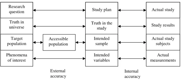
From the general definition of accuracy as a measure of to what extent a process measures what it is intended to measure (qualitatively and quantitatively), many different kinds of accuracy and systematic errors can be identified. In the planning of a medical study there should be concern about the external and internal accuracy, respectively. The external and internal accuracy are schematically illustrated in Figure 4.

The three columns in Figure 4 represent the real world, the study plan, and the performed study, respectively. In the first column there is a wish to get knowledge of a phenomenon in a population in the real world. This leads to the formulation of a research question. By practical reasons the entire target population is not studied. Often a sample is drawn from a population that is easy accessible.

The second column is the theoretical construction of a study to find the answer of the research question. There is an intention to measure some specific variables (reflecting the phenomenon in the real world) on a theoretical sample drawn from the accessible population.

The third column is the study performed, that is, where the study plan is realized. Some measurements are performed on the actual study subjects and results are obtained. Now, if everything works out good, the real study can be performed correspondingly to what was intended in the study plan. Inferences can then be made from the study results obtained on the actual sample to the intended sample (internal accuracy). If the study plan is well constructed

(22)

to investigate the phenomenon in the real world and the intended sample reflects the accessible population, the conclusions from the study can be further generalized to this population (external accuracy). If the accessible population further represents the target population in a justifying way, the conclusions can also be generalized to the target population (external accuracy). (Hulley et al. 1988)

The external accuracy is concerned with the questions: Does the study plan answer the research question?

Is what is stated as “truth” in the study plan possible to generalise to the universe outside the study?

Does the intended sample reflect the accessible population the sample was drawn from? Does the accessible population reflect the target population?

Are the variables intended to measure good measures of the phenomena of interest? The internal accuracy is concerned with the questions:

Is the actual study performed in accordance with the study plan? Do the study results support what is stated as “truth” in the study? Do the study subjects reflect the intended sample?

Do the measurements performed in the study measure the intended variables (quantitatively and qualitatively), keeping errors of measurement small?

Different forms of accuracy can be put into the main categories external and internal accuracy, respectively. The way to choose the study sample (stratified sampling, cluster sampling, et cetera) is important to get a sample that reflects the accessible population (external accuracy). Content accuracy is a measure of to what extent the items on a test are representing the knowledge wished to investigate (internal accuracy) (Dawson and Trapp 2001).

Other kinds of accuracy may not easily be fitted into the categories external and internal accuracy. Criterion accuracy is a measure of the ability to use the measurement to predict other characteristics related to the measure and cannot easily be defined as either external or

Accessible population

Figure 4. Schematic illustration of external and internal accuracy. From Hulley et al. (1988).

External

accuracy Internal accuracy Research question Truth in universe Target population Phenomena of interest Actual study Study results Actual study subjects Actual measurements Study plan Truth in the study Intended sample Intended variables

(23)

internal accuracy. The construct accuracy is estimated by showing that the used instrument (for example measuring quality of life) is related to other instruments measuring the same characteristic (for example SF-36), and not related to other characteristics (Dawson and Trapp 2001). This is not strictly either external or internal accuracy. The construct accuracy is probably more relevant in survey research than in more “technical” measurements. Still, it is easy to see the parallels to technical measurements where the results are compared to a gold standard, to evaluate accuracy.

Precision can be defined as a measure of the spread or the measurements without reference to the results agreement with the true value. From this definition different kinds of precision and random errors can be identified depending on the cause of the error. Intrarater precision reflects the lack of variability when the same observer repeats the measurements with the same instrument (Dawson and Trapp 2001). This (lack of) variation within the same observer and measuring instrument is by other authors referred to as repeatability (Rabinovich 1995). Interrater precision reflects the lack of variability when different observers repeat the measurement with the same instrument (Dawson and Trapp 2001). This (lack of) variability is also called reproducibility. Reproducibility is also used as a wider concept including variation between raters using different instruments, variation between different laboratories, et cetera (Rabinovich 1995). The different kinds of precision discussed above are possible to estimate for both laboratory and paper scale measurements. For paper scales there are also test-retest and internal consistency precision. Test-retest precision is a measure of the scales ability to reproduce the same measurements on different occasions. By practical reasons this can be hard to administer, and therefore the internal consistency precision is sometimes used as an estimate of the test-retest precision. The internal consistency precision of the items on a scale is a measure of how closely correlated the items are to each other, that is, to what extent the items measure the same characteristic. (Dawson and Trapp 2001)

Measurements and errors at orthopaedic workshops

The everyday work at an orthopaedic workshop is highly dependent on qualitative and subjective judgements and the experience of the individual CPO. The experience of examination of patients and production of prostheses and orthoses is hard to communicate to less experienced colleges. This has resulted in a practice at the orthopaedic workshops where the novices can get advice from the more experienced CPOs, but have to learn very much through trial-and-error. The disadvantage of trial-and-error is that it is very time consuming and many patients are bound to get a suboptimal treatment meanwhile.

Standardisation and mechanisation of methods are important to reduce the errors due to the observer, that is, the CPO taking the measures, doing the casting or the rectification, et cetera. The measuring instruments should also be improved to reduce errors. For example may different measuring-tapes give different results. CAD/CAM systems using a laser beam to scan stumps are examples of mechanisation of the casting process, which normally is highly subjective. When the process is less bound to specific persons and instruments, persons and instruments can be exchanged, which makes the process more flexible. For example can another person than the specific CPO does the rectification of the limb model after measurements taken in a standardised manner. Today, measures taken on the patient are so highly influenced by the CPO (and maybe the measuring-tape) that it may be hard for other persons to use them in the production, in case the CPO gets ill, is on holiday, et cetera. Less personal and instrumental influence also makes it possible to localise the whole production somewhere else (central production). A more mechanised procedure is also easier to learn to

(24)

perform to the inexperienced CPO. The success of the work is then less dependent on gained experience. The trail-and-error period may then be reduced and fewer patients get a unsatisfactory treatment caused by the inexperience of the CPO. Further, if errors of measurement are evaluated for the standardised methods the material in the CPOs’ journals can be used in scientific studies. Today, many of the measurements performed at orthopaedic workshops have not been evaluated when it comes to errors of measurements, or at least the results are unknown among CPOs.

The crucial question is how the experience and qualitative knowledge of the clinically active CPOs can be transformed into more standardised, mechanised, and quantifiable methods. This development work should preferable be performed by persons with technical knowledge and insight in errors of measurement in cooperation with experienced CPOs.

The focus in this thesis is the quantification of the volume changes after an amputation. Although several factors influence the decision of when to fit with definitive prosthesis, the quantification of volume would at least make the “volume factor” less subjective. Before the method to assess stump volume can be recommended for clinical use it is necessary to evaluate its errors of measurement.

(25)

AIM

The aim of the present study was to evaluate accuracy and intra- and interrater precision of a method to assess residual limb volume from circumferential measurements when used on transtibial stumps.

(26)

MATERIAL AND METHODS

Study design

The study consisted of two parts, the first part assessing accuracy and the second part assessing intra- and interrater precision of the method to use circumferential measurements for volume determinations.

Volume determination

Determination of volume using circumferential measurements

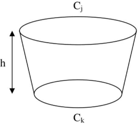
A technique to assess residual limb volume from circumferential measurements was described and used on transfemoral stumps in an article by Krouskop et al. (1979). The method approximates the stump as a number of cut cones and the stump tip as a tip of a sphere. The only measurements required are circumferences measured at regular intervals and the height of the stump tip. The assumptions in this method are that any two successive cross sections are parallel and circular and that the volume contained between them can be approximated as a right cut cone. The volume between two cross sections can then be approximated by the formula: π 12 C * C C C h* V₌ j2 + k2 + j k [8]

Were h is the distance between the two cross sections and Cj and Ck are the circumferences at

the two sections, respectively, Figure 5.

Further is the volume of the stump tip approximated as a segment of a sphere. The volume can then be estimated by the formula:

π 8 C * t 6 π * t tip V 2 3 + = [9] Cj Ck h

(27)

Were t is the height of the segment and C is the circumference at its base, Figure 6. The total volume of the stump is calculated by adding all the incremental volumes and the volume of the tip. In the present study the volumes were calculated with either a programmable

calculatora_{(Casio fx-7700GE) or a simple program written in Microsoft Excel.}

Determination of volume using CAPOD

The CAPODb system is a CAD/CAM system developed for prosthetics and orthotics. It

consists of a laser scanner unit, CAD software for design rectification of the scanned objects, and a milling machine. The CAPOD system has been described in detail in an article by Öberg et al. (1989).

Volume calculations were performed by taking values of circumferences and distances in the

software and substitute them into the formulas [8] and [9]. The software also gives

information about the volume contained within any two limits on the scanned stump. This volume was used as a reference, a gold standard, to compare the calculated volumes to.

Accuracy

The first part of the study, assessing accuracy of the method, was divided into three steps considered with theoretical accuracy of tip volume, theoretical accuracy of stump volume, and practical accuracy of stump volume, respectively.

Theoretical accuracy of tip volume

In the first step the aim was to choose the best site for taking the last circumferential measurement, that is, to choose the height of the tip, t, Figure 6. Six residual limb models were scanned with CAPOD and circumferential measurements were made inside the software, Figure 7. Comparisons were made between tip volumes calculated by the software calculated and tip volumes calculated from circumferential measurements. Comparisons were made between taking the last measurement at five respectively four cm from the distal end of the stump.

Figure 6. Approximation of stump tip volume as a sphere segment.

C t

(28)

Theoretical accuracy of stump volume

In the second step, measurements made in the software were used to calculate the whole residual limbs. These volumes were compared to the volumes calculated by the software. As a start the circumferences were measured five cm apart, that is, h = 5 cm. If not an acceptable accuracy could be obtained the procedure was repeated with h = 4 cm and with h = 3 cm, respectively. The limit for an acceptable accuracy was set to ±5% of the reference volume, that is, the volume calculated by the software. 5% is approximately the volume of one stocking (Lilja and Öberg 1997).

Practical accuracy of stump volume

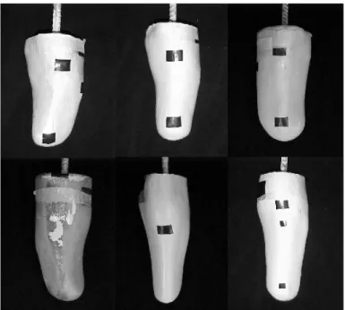
In the third step the second step was repeated in reality on the residual limb models, Figure 7. Every model was measured manually five times by the author with h = 5 cm. The procedure was then repeated with h = 4 cm and h = 3 cm, respectively, if an acceptable accuracy could not be obtained with h = 5 cm. The same criterion for an acceptable accuracy was used as in the second step. The volumes of the models had previously been assessed in studies using a water immersion technique. These volume determinations were used as reference volumes to compare the calculated volumes to. The volumes of models 1-3 had been determined by Johansson and Öberg (1998) and the volumes of models 4-6 had been determined by Lilja and Öberg (1995).

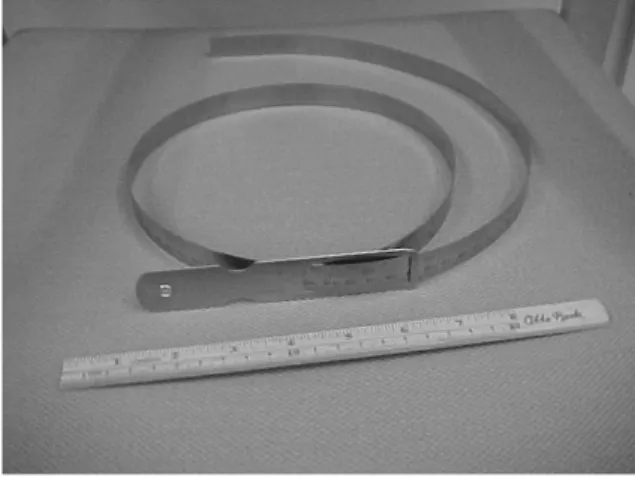
An Otto Bock wooden rule and a metal circumference rulec were used for the measurements,

Figure 8. The wooden rule was 20 cm long and had a resolution of 1 mm. The circumference rule was 16 mm wide and could show circumferences with a resolution of 0,1 mm, but in this study a scale with a 1 mm resolution was used and all measurements were rounded off to the closest mm. The metal circumference rule was used instead of the flexible measuring-tape used by CPOs clinically because the circumference rule can easily be disinfected, which is an

Figure 7. Residual limb models 1-6. Anterior view.

(29)

advantage if the stump has unhealed wounds. Another advantage is that the circumference rule has a construction that makes it easier to measure the circumferences in one plane without twisting the rule.

Precision and sources of error

The second part of the study, assessing precision, was divided into two steps. In the first step the method was used on transtibial residual limbs and intra- and interrater precision were calculated. In the second step the results were analysed to find the sources of the errors.

Measuring procedure

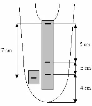
Four CPOs measured eight transtibial stumps in a randomised order, Figure 9. The same kind of equipment was used as when assessing accuracy, Figure 8. The rating CPO measured every stump five times before measuring next stump. Before the measuring began a tape with a pen mark was put on the stump by the author seven cm distal from the anterior, proximal end of tibia, Figure 10. A thin nylon stocking was then put on the stump to protect the skin from the wear and tear of the repeated changes of tapes.

(30)

Every CPO was given written instructions for the measurements, telling them to ask to patient to sit with their knees extended and muscles relaxed during the measuring, Appendix I. The CPOs were also given forms to fill in with the results, Appendix II. The CPO put an adhesive tape along the tibial crest and made a mark four cm from the distal end of the stump, Figure 10. Marks were then made every five cm going distal from the anterior, proximal end of tibia. When less then five cm was left to the first mark, the distance was recorded and filled in the form. Circumferential measures were taken by every mark and also filled in the form. A measurement was also made by the mark seven cm distal from the proximal end of tibia. Last, the tape at tibia was removed. This whole procedure was repeated for every measurement. In this way the proximal tibia and the measuring sites had to be identified for every measurement. The tape seven cm distal from proximal tibia was never removed, this mark was “constant” during the whole measuring session. Comparisons could then be made between the precisions of the circumferences when the site had to be identified by palpation and when a given site was used.

(31)

Intrarater precision

The intrarater precision was estimated in two ways: by calculating the ICC and by calculating the number of measurements within acceptable error limits. The limit for an acceptable ICC was set to 0,85. An acceptable error was considered to be ±5% of the true volume. The clinical criteria for an acceptable intrarater precision were: 1) at least 95% of the measurements within the ±5% limit and 2) no more than one unacceptable volume estimation per stump. The intrarater precision was calculated for every CPO individually.

The ±5% limit used for the evaluation of precision was based on the assumption that the systematic error was zero, or could be fully corrected for. The total error, which should not exceed ±5%, would then only consist of the random error.

As the true volumes of the stumps were not known the mean of the five volumes calculated by each CPO was calculated and used as a reference volume for that CPO on that stump. While the systematic error was assumed to be zero, the mean of repeated measurements would be the true volume. The means and error limits were calculated in the same manner for all stumps and repeated for all CPOs.

Interrater precision

The interrater precision was correspondingly estimated in two ways: by calculating the ICC and by calculating the number of measurements within acceptable error limits. Again the limit for an acceptable ICC was set to 0,85. The clinical criterion for an acceptable interrater precision was that all volumes assessed by the CPOs should be within the error limits, that is, ±5% of the true volume. While the true stump volume was not known the mean of all 20 measurements made on each stump (four CPOs measured every stump five times each) was assumed to be the true volume.

Each CPO’s fifth measurement on each stump was used in the analysis. The fifth measurement was chosen to avoid errors due to introducing problems with the measuring