Winner Prediction of Blood Bowl 2 Matches with Binary Classification

(1)

Master Thesis Project 15p, Spring 2019

Winner Prediction of Blood Bowl 2 Matches with

Binary Classification

By

Andreas Gustafsson

Supervisors:

Jose Maria Font Fernandez

Alberto Enrique Alvarez Uribe

(2)

Contact information

Author:

Andreas Gustafsson

E-mail: andreasgustafsson95@gmail.com

Supervisors:

Jose Maria Font Fernandez E-mail: jose.font@mau.se

Malmö University, Departament of Computer Science

Alberto Enrique Alvarez Uribe E-mail: alberto.alvarez@mau.se

Malmö University, Departament of Computer Science

Examiner: Johan Holmgren

E-mail: johan.holmgren@mau.se

(3)

3 Preliminaries: Blood Bowl 2 28 3.1 Terminology . . . 28 3.2 Description . . . 28 3.2.1 Statistics . . . 29 3.2.2 Races . . . 29 3.3 Examples of Playing . . . 35 3.4 Community Aspects . . . 38 4 Proposed Approach 40 4.1 Considerations . . . 40 4.2 Data Generation . . . 41 4.3 Features . . . 41 4.4 Datasets . . . 44 5 Method 48 5.1 Motivation . . . 48 5.2 The Experiment . . . 49 5.3 Measurements . . . 50 5.4 Classifiers . . . 50 5.5 Hyper-Parameter Search . . . 52 6 Result 53 6.1 Classification Performance . . . 53 6.1.1 Base Dataset (D1) . . . 55

6.1.2 Dataset with Races (D2) . . . 58

6.1.3 Dataset with Play-styles (D3) . . . 61

7 Analysis and Discussion 64 7.1 Classification Performance and Datasets . . . 64

(5)

8 Conclusions and Future Work 68 8.1 Conclusions . . . 68 8.2 Future Work . . . 69 References 71 9 Appendix A 79 9.1 Replication Data . . . 79

(6)

Abstract

Being able to predict the outcome of a game is useful in many aspects. Such as, to aid designers in the process of understanding how the game is played by the players, as well as how to be able to balance the elements within the game are two of those aspects. If one could predict the outcome of games with certainty the design process could possibly be evolved into more of an experiment based approach where one can observe cause and effect to some degree. It has previously been shown that it is possible to predict outcomes of games to varying degrees of success. However, there is a lack of research which compares and evaluates several different models on the same domain with common aims. To narrow this identified gap an experiment is conducted to compare and analyze seven different classifiers within the same domain. The classifiers are then ranked on accuracy against each other with help of appropriate statistical methods. The classifiers compete on the task of predicting which team will win or lose in a match of the game Blood Bowl 2. For nuance three different datasets are made for the models to be trained on. While the results vary between the models of the various datasets the gen-eral consensus has an identifiable pattern of rejections. The results also indicate a strong accuracy for Support Vector Machine and Logistic Regression across all the datasets.

Keywords: Machine learning; Blood Bowl 2; Predict winner; Outcome predic-tion; Supervised learning; Binary classificapredic-tion; Match prediction.

(7)

Popular Science Summary

Can the computer predict who will win a match of Blood Bowl 2? Yes! 88% of the time it will correctly guess which team will win a match of the game. This is important since it shows that given enough time to test many different settings and algorithms accurate guesses can be made for complicated games like Blood Bowl 2. If we document what has been tried and how it went for many different problems then it will be easier to understand what algorithms to start trying with at a new problem that is similar to other problems that have already been done.

This discovery is good for the curious player community of Blood Bowl 2, as many of them try to understand the game even better. It is also good for people to get a starting point at ideas that might work for their own similar problems.

If we manage to accurately guess who will win in games it will help a lot during the development of new games. The creators will be able to test new things quickly to see how it changes their game instead of having to let the players of the game act as test subjects for their new ideas.

How can the computer guess so well? It looks at matches played by players before and find similar matches to the one that is about to be played. If it has enough knowledge about how the similar matches went it will make an educated guess about how this match will go.

(8)

Acknowledgement

Special thanks to Jose Font and Alberto Alvarez for all the supervision, feedback, and excellent help during times of confusion. Also, many thanks to Carl Magnus Olsson for introducing, and coaching me through, the world of Blood Bowl. Finally, thanks to everyone over at the Blood Bowl community that helped out with various questions with unyielding support.

(9)

List of Figures

2.1 Illustration of a decision tree (DT) . . . 21

2.2 Illustration of the main idea behind a Support Vector Machine (SVM) 23 2.3 Illustration of k-Nearest Neighbors (kNN) . . . 25

2.4 Illustration of a multilayer perceptron (MLP) . . . 27

3.1 Illustrations of all races in Blood Bowl 2 . . . 35

3.2 Bird view of Blood Bowl 2 playfield . . . 36

3.3 Start of a match in Blood Bowl 2 . . . 37

3.4 Active turn in Blood Bowl 2 . . . 37

3.5 Showing a player carrying the ball in Blood Bowl 2 . . . 38

6.1 Plot of accuracy of classifiers from D1 . . . 55

6.2 Plot of accuracy of classifiers from D2 . . . 58

(10)

List of Tables

4.1 Example of general rows in the dataset . . . 46

5.1 Section index of Classifiers . . . 51

6.1 Accuracy of classifiers from D1 . . . 56

6.2 Statistical relevance of comparisons for classifiers from D1 . . . 56

6.3 Confusion matrix of Dummy model for D1 . . . 57

6.4 Confusion matrix of the Gaussian Naive Bayes model for D1 . . . . 57

6.5 Confusion matrix of the Decision Tree model for D1 . . . 57

6.6 Confusion matrix of the k-Nearest Neighbors model for D1 . . . 57

6.7 Confusion matrix of the Support Vector Machine model for D1 . . . 57

6.8 Confusion matrix of the Logistic Regression model for D1 . . . 57

6.9 Confusion matrix of the Random Forest for D1 . . . 57

6.10 Confusion matrix of the Multilayer Perceptron for D1 . . . 57

6.11 Accuracy of classifiers from D2 . . . 59

6.12 Statistical relevance of comparisons for classifiers from D2 . . . 59

6.13 Confusion matrix of Dummy model for D2 . . . 60

6.14 Confusion matrix of the Gaussian Naive Bayes model for D2 . . . . 60

6.15 Confusion matrix of the Decision Tree model for D2 . . . 60

6.16 Confusion matrix of the k-Nearest Neighbors model for D2 . . . 60

6.17 Confusion matrix of the Support Vector Machine model for D2 . . . 60

6.18 Confusion matrix of the Logistic Regression model for D2 . . . 60

6.19 Confusion matrix of the Random Forest for D2 . . . 60

6.20 Confusion matrix of the Multilayer Perceptron for D2 . . . 60

(11)

6.22 Statistical relevance of comparisons for classifiers from D3 . . . 62 6.23 Confusion matrix of Dummy model for D3 . . . 63 6.24 Confusion matrix of the Gaussian Naive Bayes model for D3 . . . . 63 6.25 Confusion matrix of the Decision Tree model for D3 . . . 63 6.26 Confusion matrix of the k-Nearest Neighbors model for D3 . . . 63 6.27 Confusion matrix of the Support Vector Machine model for D3 . . . 63 6.28 Confusion matrix of the Logistic Regression model for D3 . . . 63 6.29 Confusion matrix of the Random Forest for D3 . . . 63 6.30 Confusion matrix of the Multilayer Perceptron for D3 . . . 63

(12)

List of Acronyms

ANN Artificial Neural Network DT Decision Tree

FN False Negative FP False Positive GFI Go For It

GNB Gaussian Naive Bayes ID Identification

JSON JavaScript Object Notation kNN k-Nearest Neighbors

LR Logistic Regression MLP Multilayer Perceptron MVP Most Valuable Player PM Player Model

RF Random Forest

RMSE Root Mean Square Error RQ Research Question SVM Support Vector Machine TN True Negative

(13)

Chapter 1 Introduction

This section is dedicated to introducing the study by first presenting motivation for the study and framing of the domain. After that, the aim and objectives are explicitly told, followed by definition of the research questions to be explored in the paper.

1.1 Motivation

There are several aspects of interest when it comes to discovering what types of problems can be solved with help of machine learning techniques[1], [2]. For this paper there are especially two aspects that will be looked into, namely the way to gain further knowledge about games and players, and the interests of how to create accurate prediction models for game outcomes. The reason behind looking into both of them are due to how can be seen as intertwining with one another.

Many studies have utilized machine learning to gain further insight about how the game in question is played by the players[3]–[8]. It is of great interest for game designers to have this form of information as guiding help when making decisions

(14)

learning techniques[10]–[18]. Some, such as De Pessemier et al., go even further than predicting outcomes of a match by even including the approach of money management and which kind of outcomes are better or worse to trust by building an application meant to assist in many parts of the betting process rather just the outcome prediction[18].

To further explain the previous statement about how one can see these aspects as intertwining and complement each other it is asked of the reader to consider the following; one needs some form of knowledge about the players and of the game itself to be able to predict outcomes within the domain of it. Likewise, if it is possible to predict outcomes of a game this will inherently lead to further understanding and guidance within the design process of the game. Imagine, for example, that a new mechanic is introduced in a game. If you are able to predict outcomes of the game before, and after, the introduction of said mechanic you are able to see how it will affect the game itself as a cause and effect relation. With this in mind as motivation for the research the goals are presented in section 1.3. Finally, to further motivate the choice of the game “Blood Bowl 2” as domain for the study one can look at the growing interest in the specific game series from a research perspective. This interest originates mostly from the complex nature of the rules the game provides[19].

1.2 Aim and Objectives

While many different machine learning approaches have been applied to many different games with the intent to accurately predict outcomes the results are varying heavily between the studies[12]–[18]. It is our understanding that there is an infrequency of research further evaluating multiple different models to predict the outcome for a specific domain. This identified gap gives rise to the desire of constructing, evaluating, and analyzing multiple models of various kinds within the same domain to then compare the results of the models.

In other words, the aim of this study is to explore how different prediction models perform in the same domain, and to be able to compare the models with each other successfully. It is our intention to start providing an overview of what kind of model worked better or worse for the domain in question, in hopes that it

(15)

will prove fruitful and spark more similar research within various domains, which could ultimately lead to a more composed and structured picture of analysis over how well different models perform for different games.

In order to accomplish the aim of the study the following goals have been established:

• Examine existing methods for outcome prediction in games; identify feature engineering strategies and feature selection techniques.

• Analyze the domain and dataset available.

• Perform feature engineering and select feature selection techniques deemed suitable for the task at hand.

• Implement the models to be tested.

• Run experiments to evaluate the performance of the models.

• Compare the model results against each other with statistical analysis. • Analyze the results.

1.3 Research Questions

The following research questions have been set out for this study:

RQ1 How can machine learning models for classification be used to predict match outcomes in the digital game Blood Bowl 2?

RQ2 How does the classification performance differ between different types of prediction models?

(16)

The first research question examines how various machine learning models can be used to predict outcomes in the specific domain. It considers how the selected models parameters can be (1) used to their advantages for the study, and (2) what kind of prediction strategy should be employed. Examples of prediction strategies could for example be that of identifying various player types to aid prediction; or to look at historical or play styles of the contestants; or even a combination of the two.

The second research question focuses on the results of the tested models. This is the question that drives the statistical analysis and comparison of the models forward. In other words, this is the question that shows if the answers found are of statistical relevance, as well as giving a structured overview of performance.

The third research question is the leading motivator to look further into the vast domain of blood bowl and the contributions already made within it to further understand the underlying complexity of the game. This will be explored further by making use of properly established play styles from the domain experts of the community.

Finally, the fourth research question can be seen as what binds the previous questions together by focusing on how the expert knowledge actually affects the models and in what ways.

1.4 Expected Outcome

The expected outcome of this study is to provide deeper knowledge about the inner complexity of matches in the game Blood Bowl 2. For example, to be able to see more clearly if the play style categories created by domain experts say more about the outcome of a match; or if looking at the various races of the players tells more of it; and so on.

By creating models that may be able to accurately predict the outcome of the matches we can establish that there are important patterns at play, and get some insight into those patterns themselves. By highlighting this further knowledge and understanding about the game is hoped to be achieved, which could in turn bring further material for the community of the domain to analyze and dwell deeper into.

(17)

1.5 Summary

This section framed the study while also showing the motivations for why it is worth conducting both for the sake of academia as well as the concerning domains community. Together with the aims and objectives set out for the study the research questions were explicitly stated, together with proposed ways of reaching answers for them.

(18)

Chapter 2 Related Work

This chapter is dedicated to presenting the state-of-the-art for machine learning, and showing how it can be useful for outcome prediction of matches in complex domains such as the digital game Blood Bowl 2[19], [20]. Some of the terminology needed to be understood for the remainder of the study will also be explained here.

2.1 Outcome Prediction

To create models that predict the outcome of games is nothing new in itself, it has been done as early as in the 1980s[21]. The motivation to predict outcomes is plenty-fold. For example, it may be with the goal of wanting to be able to design better artificial intelligence opponents[12], [15], [17]. It could also be with the goal of financial success by betting[18], or simply due to wanting to solve a complex problem[14].

There is still a large variation of success rates for different studies about pre-dicting outcomes of complex games. For example in [16] it is reported to have achieved an accuracy of 57.7% for soccer, while [14] report having achieved above 70% accuracy on their Dota2 predictor. The three papers [12], [15], and [17] competed in the same tournament. Cen et al.[12] reported having a root mean squared error (RMSE) of 5.65% achieving the 2nd place in the tournament, while [15] achieved 6.35% thus getting 10th place, and [17] won the contest, however they did not state their RMSE percentage.

(19)

Since both the models and the domains are different in most of the cases reviewed it is difficult to get an overview of what techniques work better than others for certain kinds of domains. It is due to this that we propose the notion of evaluating multiple different models under the same problem domain. This argument can be further realized by the notion that the three publications ([12], [15], [17]) from the same tournament utilize rather different approaches instead of having a common starting ground as is seen by more well known problems.

2.2 Player modelling

To construct a computational representation of a specific player based on their current, or historical, behaviour in one or more game sessions is to create a so called player model (PM) [22]–[24].

There are three categories of different types of data to consider when construct-ing PMs; (1) gameplay data, (2) objective data; (3) game context. The first type is about the actual behaviour of the player while playing the game, such as if the player decides to pick alternative A or B at a branching choice. The second type is strict measurements carried out about the player, such as their eye movement or perspiration, and so on. The third type is about the in-game domain itself, such as the amount of rooms in a dungeon, the various missions available, and so forth[22].

Traditionally, the model constructed of the player is used to change the game play experience to be more suitable for players in regards to their personally con-structed player model [22], [23]. However, one could argue that both the data used in this study, and the utilization of it for further game knowledge, fulfill the requirements to be seen as player modelling. Although, rather than using the con-structed PM to dynamically change the player experience in some way it is used to predict outcomes of matches in the game. One could say that the prediction

(20)

classification is the same thing, however it does point out an overlap of the areas.

2.3 Machine Learning

Machine learning (ML) is about solving problems that are in some form intuitive to people, but that are hard to describe in a formal manner. By letting the computer build up a world view in a manner of relating data to one another and finding patterns the computer learns to understand complicated concepts. In other words, the computer gradually builds an understanding of concepts instead of having the need of a human explaining every relation and detail of said concepts[25].

A more formal way of expressing what machine learning is can be as Goodfellow et al.[26] puts it when writing “Machine learning is essentially a form of applied statistics with increased emphasis on the use of computers to statistically estimate complicated functions and a decreased emphasis on proving confidence intervals around these functions...”

To further emphasize, machine learning is mainly used to identify formal pat-terns that may not be easy for a human to identify, since we lack the structured computational power of a computer. By identifying patterns in complex situations it is possible, with varying degree of confidence, to point out what kind of situation is presenting itself due to having seen similar patterns in past data.

2.3.1 Supervised Learning

We often group classification problems into two categories. These categories are called “supervised learning” and “unsupervised learning”. The difference between the two are whether or not we specify a target variable in the data which acts as the domain our machine should learn about[27].

To give an example of supervised learning; this is what will be utilized in this study. The reason for doing this is thanks to how we are able to label the data we have for our model. While the data first retrieved from the matches are not labeled we can perform operations on the information about goals done per team per match to see which coach won the given match. After having done this for all the available data the problem falls within the scope of supervised learning.

(21)

In short, supervised learning is when we have labels for the data. 2.3.1.1 Binary Classification

While classification is the task of identifying what label some feature vector in a label space belongs to, binary classification is the idea of the vector belonging to one out of two possible labels. Since only two possible labels exist the base is binary, which holds true to the name[28].

To exemplify binary classification we can imagine a situation as taking a test where you can either pass or fail; or to pick a team in chess, in other words, either white or black; or even further, either winning or losing a match of a game.

In short, binary classification is when there are only two choices to classify something within.

2.3.1.2 Decision Trees

Decision trees (DTs) have been recorded as the most commonly used classification method [29]. It is easy to explain the approach of decision trees in layman terms. As a child you might have played a game called “Twenty Questions”. The objective of the game is heavily related to the name. One person thinks of an object, and the other players are allowed to ask twenty yes-or-no questions to figure out what object the other person is thinking about. This game works in the same manner as decision trees do. In other words; asking questions to successfully split the set of potential objects the data given could be. One very desirable trait of the decision tree is that they are easily read and understood by people [30].

To further describe; a decision tree has nodes that ask questions, different edges to travel down depending on the answer of the node, and leaf nodes which show the conclusion reached. Figure 2.1 is lent from [30] and depicts a system classifying email.

(22)

Figure 2.1: A decision tree in flowchart form, concerning email where rectangles are decision nodes, and ovals are leaves[30].

2.3.1.3 Ensemble Methods

Ensemble methods are methods that combine several predictors, built with a spec-ified learning algorithm, to improve generalizing aspects and robustness of the predictor compared to if it was just a single predictor in use [31].

An example of an ensemble method used in the litterateur is that of random forests (RF). It was used as a supervised learning technique which produced good results in two papers with similar goals[13], [18]. The basic idea of random forests can be seen as a way of making decisions by counting votes of many different decision trees. The decision with the most votes is seen as the most correct one. Each of the decision trees are created with a subset of the attributes used for the forest as a whole. This idea can also be used with regression[32]. Random Forests and Random Forest Regression was tried and gave the most promising results in

(23)

[18] and [13], respectively, which make this model into a interest of exploration. Other interesting ensemble models were found in the papers [15], [12], and [17] which are all about different entries into the “AAIA Data Mining Competition 2018”. Both [12] and [17] used some form of ensemble method and performed well, getting a placement of second, and first in the tournament, respectively. Due to the different purpose of this study and the ones just mentioned it is not seen fit to try to re-use their findings completely, however it is good to keep in mind that those who utilized ensemble models proved to perform better in this specific domain.

Another well performing ensemble model is proposed by [14] for predicting results in the digital game Dota 2. An especially interesting point lifted up by this paper is how the usage of Recurrent Neural Networks are promising due to being sequential which is a good fit with match history data of individual players since that is also of sequential nature.

2.3.1.4 Support Vector Machines

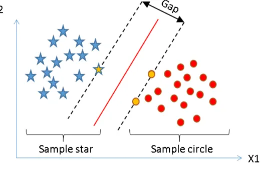
Support vector machines (SVMs) are about finding the separation between classes so that the gap between them is maximized. If the data is non-linear one can use various different kernel operations to convert the data into a higher dimension feature space to be able to find a linear separation [13]. To summarize, this means that support vector machines are good at separating extremes, while not neces-sarily adhering to the other parts of the training data for classification. See figure 2.2 for a visual illustration.

In [13] support vector regression is one of the better performing models used, being ranked number two behind random forest regression. Likewise, in [14] a support vector machine is utilized as a comparison to see how well their own model performs.

(24)

Figure 2.2: An illustration of the idea behind a SVM. Here the gap is identified as the separator between the two classifications (or labels) called “Sample star” and “Sample circle”[33].

2.3.1.5 Naive Bayes Methods

Naive Bayes methods are methods which utilize the Bayes theorem, but in a naive way by assuming some things. The first assumption is that of statistical Indepen-dence. In other words, to assume that one feature is just as likely to appear by itself as next to other features. The other assumption made is to believe every feature to be of equal importance. To exemplify what has just been said; if we see words as features the word “banana” is believed to be equally likely to come after the word “nuclear” as any other word. It is also believed that the word “banana” is as important as the word “nuclear” for what ever our model is trying to accomplish. While these assumptions do not hold true in reality the classifiers perform well in practice [34], [35].

Since naive Bayes methods are of probabilistic nature one can see it as a method that bets on what it believes to be the most likely class for the situation when it is tasked with classifying some data[34].

(25)

2.3.1.6 k-Nearest Neighbors

To explain k-Nearest Neighbors (kNN) we first have to imagine a set of data which will be our training data. Each vector of this training data has a given label; this means that we know what label each vector of data belongs to. As a label-less vector of data is given we compare it to every training data vector we have. Those that are most similar to the label-less data get to participate in a majority-vote for what kind of data this new vector belongs to. The “k” from the name kNN originates from the constant that is used to determine how many of the most similar data vectors that get to participate in the voting. For example, if k = 10 it means that the 10 most similar vectors will be looked at. The label which is in majority out of those 10 vectors is what the label-less vector shall be labeled as [36], [37].

(26)

Figure 2.3: An illustration of kNN; here the black “x” is being labeled as belonging to the red dots having the label “ω1” due to being closer to a majority of that label compared to any other label[38].

2.3.1.7 Logistic Regression

Regression is when a best-fit line is fit for some data points. Logistic regression (LR) is about creating an equation which manages to do desirable classification for its purpose. It does so by finding a good best-fit set of parameters. The output of logistic regressions is either 0 or 1, which is used to determine some class. Since a sigmoid function is often used, which gives a continuous value between 0 and 1 as answer; we see anything above 0.5 as 1, and anything below 0.5 as 0[39].

The input to the sigmoid function is a set of weights and corresponding vectors which together give an output. The trick is to find the best weights for each vector

(27)

so that the classifier becomes optimally successful. One popular way of finding the values are by what is called “gradient ascent”; which can be imagined and visualized as moving along the direction of the gradient until the stop condition is fulfilled. The stop condition is usually either a set amount of steps, or that the algorithm is within a certain tolerance threshold[39].

It is worth noting that gradient ascent and gradient descent are basically the same idea, with the exception that the plus sign of gradient ascent has been changed into a minus sign to become gradient descent. This also means that it will move along the direction of a minimum rather than a maximum[39]. 2.3.1.8 Multilayer Perceptron

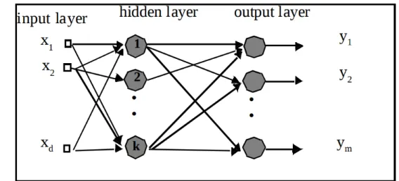
The multilayer perceptron (MLP) is a type of artificial neural network (ANN). The basic structure of a MLP can be seen as (1) “input layer”, which takes some data, (2) “output layer” that makes a final decision and outputs it, and (3) a non-fixed number of “hidden layers” in between the aforementioned two layers which are capable of approximating continuous functions. [40]–[42].

To further specify the shape of the MLP we can use terms found when talking about graphs. Firstly, MLP is fully connected, which means that each node in a layer is connected to every node in the following layer. Secondly, the MLP is layered, as seen in the fact that there are at least three layers (output layer, one hidden layer, input layer). Finally, the connections of the MLP are always directed forward, which makes it into a feed-forward graph [42].

(28)

Figure 2.4: An illustration of a MLP; here three layers are illustrated, namely the input layer, one hidden layer, and the output layer. It is worth noting (as shown by (xd, k, ym) that the number of inputs, nodes, and outputs may vary. Finally, it is once more stressed that a MLP can consist of more than one hidden layer, and that there are weights (not shown on in the figure, but can be imagined as “on the arrows”) from the nodes of the hidden layer to the next layer. The figure is from [41].

2.4 Summary

In this section the state-of-the-art relevant to the study has been discussed. For instance, the overlap within the areas of player modelling and classification in our instance has been highlighted, while still respecting the differences them. An overview of ML has been given together with a deeper dive into the various models that will be tested in the chapter 4, and an explanation of where they stand in relation to broader terms of the field.

(29)

Chapter 3 Preliminaries: Blood Bowl 2

This chapter will present the knowledge needed about the game domain “Blood Bowl 2” to understand more about the assumptions made during chapter 4, as well as the game terminology and what kind of domain the study is working with.

3.1 Terminology

Within the Blood Bowl domain the in-game characters that play on the game field are often referred to as “players”, while the person, in real life, that is actually playing the game is referred to as the “coach”. To clarify; up until this point the study has been using the term “player” to refer to the human agent. However, from now on the human agent will be referred to as “coach”, and the virtual players in the game will be referred to as “players”.

Coach – Human agent Player – Virtual player

(30)

game is played in a turn-based fashion. The goal is to get a higher score than your opponent. You score points by getting to your opponent’s end zone while holding the ball. What has just been described can be seen as mostly the “bowl” part of the game. However, the “blood” is of equal importance. In a match of Blood Bowl players are allowed, and at times encouraged, to injure or kill each other so that the opponent’s team is weakened leading to an easier time scoring points against them.

Between the matches in the game it is possible for the coach to hire new players for their team. It is often talked about as “team value” within the community when discussing the overall price class of the team.

Due to the extensive rules of the game the curious reader is encouraged to read [43] and [44] for a better understanding of the game as a whole after reading through this chapter. Lastly, the game can be played both offline and online, depending on which mode is selected.

3.2.1 Statistics

Within the game there are four different player statistics and 24 different races which specialize in different traits that encourage various forms of play styles. This section will list the statistics and the following section (section 3.2.2) will describe the races. While it will not be described in detail it is also worth knowing that players can have different abilities which affect their capabilities in various ways.

Move Allowance shows how fast the player is. Strength shows how well the player can fight.

Agility shows the player’s ball handling and evading capabilities.

Armor Value shows how difficult it is for the player to be injured during play.

3.2.2 Races

Amazon

(31)

them harder to beat down, unless you have a team such as Chaos Dwarf or Dwarf with much Tackle. Particularly strong at low team value.

Bretonnians

Known for their excellent blitzers and cheap linemen that are typically used to foul opponents extensively. A hard team to make last over time, but quite good at low-medium team value.

Chaos Dwarf

One of the most hated races for their combination of many skills on cheap team value and good blockers, good speed and strength on the centaurs, and cheap foulers with their hobgoblins. With some luck, they become fearsome with much “Guard”, “Claw”, and “Mighty Blow” which can be devastating for any team to face.

Chaos

Not a very strong early on in team development, but over time and at high team value they become extremely scary to play against. Easy access to mu-tations is what makes them so different, and they can be made into anything from highly focused on pitch control to a pure kill team.

Dark Elves

Amazingly strong early on and also develops well, even if they are not quite as explosive as the faster elf teams. A safe to play elf team that is always dangerous to face.

Dwarfs

One of the best early team value teams, with a good mix of skills. Lack of speed is their biggest weakness, which makes positioning on the field key to success. Compared with Chaos Dwarfs, they do not have access to mutations

(32)

of Steel”. It is also worth noting that this race is sometimes called “Pro elf” within the community.

Goblins

What goblins lack in skill, they make up for in secret weapons and cheap bribes to reduce the risk of getting their weapons sent off. They are dangerous to play, often for both sides at the same time.

Halflings

The best halfling is not even on the team, as the “Halfling Chef” inducement is what gives them their edge. Having access to three tree men if they manage to get Deeproot in as star player is also a great perk. However, it is still not typically viewed as a serious team, although having more potential than often given credit for.

High Elves

Fast, agile, and with pretty good armor value. However, they start with few skills and therefore are at their best with high team value when players have had a chance to pick up more skills to help them.

Humans

The jack of all trades, master of none. They make for a good starting team with a great set of initial skills. However, with time their effectiveness drops as the more powerful teams play better power ball (as in rough plays) while the more agile teams out-dodge them.

Khemri

Often seen as a slow team, but it can be argued that speed is not their problem; as having four very strong tomb guardians mean a lot of potential to cover the ground very well. A more established weakness of the team is that it has no real skill within how to handle the ball, ranking worse in terms of ball handling potential within the whole game.

Kislev circus

Every player has “Very Long Legs” and “Leap” which provides great mobility of the playfield. However, the players are expensive and take a long time to

(33)

develop. This makes them into a force to be reckoned with when developed, but it is also very difficult to get to that point without losing matches. Lizardmen

Speed and strength, that is what Lizardmen are all about. The most im-portant players are slow to develop, while the easy ones to develop tend to die often as they are rather weak. This race is very sensitive to teams that largely bypass the high armor values on the lizardmens’ stronger pieces since if they die they take a very long time to develop again. However, as long as they survive they are a strong team.

Necromantic

Possibly the best positional player team in the game, particularly over some games, as Werewolves have speed, great statistics, “Claw”, and with the capacity to become speedy killers as well as dangerous scorers. Plays stronger in medium to high team value games compared with Undead who are at their best earlier on.

Norse

Almost every player starts with “Block”, making them extremely good early on, but having “Frenzy” on so many players can also be very difficult to manage. However, the biggest weakness to deal with, is the low armor values of the players in this race.

Nurgle

A very slow race to develop, also plays much slower than Chaos even if the two teams have very similar main players and same skill access. Their “Beast of Nurgle” is regarded as one of the best big players in the entire game. However, expect to struggle quite a few games until enough time to develop skills to help out has passed. This race can develop into a kill, or

(34)

use Gnoblars which happen to be the worst players in the game. Gnoblars are weaker than all other players, have very low armor value, and generally a hard time to develop into anything other than food for Ogres that want to “Throw Team Mate” but goes “Always Hungry” instead.

Orcs

The power version of a human team, and while they formally have a thrower, they don’t really have any catchers. The team lives entirely upon running with the ball and bashing the opponent into the ground during the process. It is a very easy-to-play and good team early on, that does well all the way up to high team value. As with other high armor teams, they struggle against teams that use the “Claw” ability. Especially the stronger “Black Orcs” are slow to develop.

Skavens

No other team has the same overall speed as Skaven does. Wood Elves may come very close in speed, but Skaven are much cheaper and thus much easier to have a full set of speedy players on. With access to mutations, Skaven may grow “Claws”; “Horns”; “Extra Arms”; “Extra Heads”; “Big Hands”; “Very Long Legs”; all of which fit perfectly into what Skaven teams do best, namely, stealing the ball and score right away.

Undead

The backbone of the Undead team is their two Mummies, but it is their Wights that often do the hard work as they are easier to develop than Mum-mies that lack access to the “Block” skill. With up to four ghouls Undead have an excellent mix of speed and brute force. The mummies in particular also carried high armor value. However, the ghouls have low armor value, but often end up developing the most only to die in the coming match. Without access to “Regeneration” like the rest of the team this can be a deal breaker for the Undead teams.

Vampire

The biggest challenge for Vampire teams is to run out of “Vampire Thrall” players to bite any time they fail their “Bloodlust” roll. The Vampires have

(35)

one of the most attractive statistics line, and also great skill access, but that does not do much good when there are no thrall players left to keep opponent teams at a safe distance; or bite, if the urge for blood arises.

Underworld Daemons

This is a mixture of a Skaven and Goblin team with easier access to mu-tations. Underworld players are extremely sensitive early on to teams with “Tackle” and “Mighty Blow”. However, once they develop their offensive play-ers into killplay-ers with “Claw”, they become lethal. Even their “Troll” mutates, so it can quickly help out cutting down opponent teams to more managable sizes.

Wood Elf

“Wardancers” are the best players in the game out of the box, as in with just their starting skills. They level very fast, and score as well as steal the ball better than any other player in the game. Combine that with the fastest catchers in the game, and big “Treeman” to hold down the center of the field and you have the definition of a “glass cannon” team. As appropriate of a “glass cannon” team it is absolutely dangerous to be up against, yet it has a tendency to die off a lot quicker than most other teams.

(36)

Figure 3.1: This figure shows all the races from Blood Bowl 2. Picture is from [45].

3.3 Examples of Playing

At the start of a match each coach has 11 players on the field, taking various positions. As previously stated, the match is played in a grid on the play field, which gets further emphasized by fig. 3.2 that is shown to help get an idea of how the game looks. The grid structure of the playfield can be further seen by focusing on the white square marker in the figure. One can also see the statistics of a player on the left of the figure.

(37)

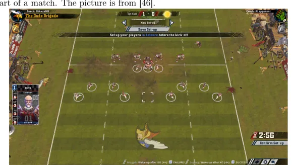
Figure 3.2: This screenshot from Blood Bowl 2 shows a setup of players before the start of a match. The picture is from [46].

After the initial setup the match begins. As this happens the coach may start to select the players of the concerning team to decide what they will do during their turn. This can be seen by looking at fig 3.3 and fig 3.4 in sequence. The first figure shows before any player has been marked and ordered to do an action, while the second figure shows the ongoing move of an ogre by the name “Blargh”. As can be seen by the dice over the ogres head, a lot of actions made by players involves chance, or risk, due to having to cast die to determine the outcome. Depending on the situation, such as how many opponents are in range of the action, or the various stats of the players concerning, the die cast can be more or less rewarding or devastating in outcome for the respective coaches.

In other words, if a player does an action close to an opponent (such as for example trying to walk past an opponent) it will trigger die casting events to

(38)

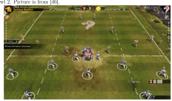
Figure 3.3: This screenshot from Blood Bowl 2 shows the start of a match in Blood Bowl 2. Picture is from [46].

Figure 3.4: This screenshot from Blood Bowl 2 shows a turn in progress in Blood Bowl 2. Picture is from [46].

A common tactic in Blood Bowl 2 is to try to protect the ball carrier from opponents by “boxing” it in with team mates. The team mates then make it more

(39)

difficult for opponents to get to the ball carrier, which means that they will have a harder time stealing the ball. An example of this strategy can be seen in fig 3.5. The player that glows blue carries the ball, while his team mates defend him from opponents trying to get “into the box” of defense.

Figure 3.5: This screenshot from Blood Bowl 2 shows the ball carrier standing in a box between his team mates protecting him from opponents. Picture is from [46].

While it is on the edge of being out of scope for this study it is worth noting that the game is not strictly limited to the matches themselves. The game has a dimension of buying players for the team; of deciding how the players of the team should specialize as they gain levels by picking out new abilities for them; of managing injuries and deaths of the players, and so on. In other words, there is a dimension of team management present in the game. However, as it is not present for the model creation of the study it is not explained in-depth.

(40)

Examples of that can be found over at [47]. The post [48] is of interest for this study as it is used as guide for play styles used as features in one version of the dataset, however more of this will be mentioned in section 4.1.

Data analysis is not the only thing the community sees to being carried out. There are several large sub-communities within the Blood Bowl 2 domain which hold their own tournaments or leagues[49]. These tournaments employ various community-made rules, such as banning specific types of play or being able to put bounties on players heads, and so on.

(41)

Chapter 4 Proposed Approach

In this chapter the general idea behind the considerations of how to solve the specified problem will be given. Do note that chapter 5 will focus on the experiment part of the study, while this chapter will focus on the parts building up to the experiment itself.

4.1 Considerations

The data can be seen as a collection of results from previously played matches of Blood Bowl 2 (further explained in section 4.2, section 4.3, and section 4.4). The problem we wish to solve with help of this data is to predict which coach will win in future matches. To be able to tackle the problem some assumptions have been made about domain.

Our first assumption is that some styles are stronger against other play-styles, which naturally also means that some play-styles are weaker against other play-styles. Similar assumptions have been made in other studies as [15] when predicting winners of Hearthstone matches.

(42)

play-style is found by taking the average behaviour of the coaches past matches.

4.2 Data Generation

When the game is played online a lot of game-play data is generated and stored. This data can be seen as log data about what that happened in a match, which includes the outcome reached. For example, the data indicated where on the field each player stands each turn. It also provides the status of each player, as well as notable things they have done (such as for example killing an opponent player or scoring a goal). The various stats and skills of each player is also saved. Moreover, the time and date of the match as well as the league name, coach names and so forth are also present. It is worth noting that the data is continuous; except for names on leagues, coaches, players, player skills, and so forth.

Since statistics such as the total number of goals; deaths; kills; passes; tackles; and so on; is saved, as well as positioning data to be able to recreate how each player moved each round during the match a situation is presented where a vast amount of data is available to the study. Thanks to having access to these large amounts of game-play data that the opportunity to create prediction models with help of machine learning has presented itself, especially when taking the community tournament aspects in consideration, which are talked about in 3.4.

4.3 Features

Blocks is a decimal value representing how many blocks have been performed, on average, by the coach.

BlocksAgainst is a decimal value representing how many times, on average, the coach has been blocked in games.

Breaks is a decimal value representing how many times, on average, the coach has made breaks against the opponent.

BreaksAgainst is a decimal value showing the average amount of times breaks have been made against the coach.

(43)

Casualties is a decimal value indicating on the average amount of casualties the coach creates per match.

CasualtiesAgainst is a decimal value indicating on the average amount of casu-alties per match for the coach.

Catches is a decimal value showing the average amounts of catches (of the ball) performed by the coach per match.

Dodges is a decimal value showing the average amount of dodges performed by the coach per match.

GFIs stands for “Go For It” and is a action in the game that lets your player move two extra squares, but has a risk of falling on each additional square traversed. This column shows the average amount of GFIs made by the coach per game.

GamesPlayed shows a decimal value indicating how many games the coaches players have played on average.

Interceptions this is a decimal value showing how many interceptions that the coach performs per match, on average.

IsActive is a decimal value to keep track of which user, players, and teams that are still active in the league and which have left or been banned.

IsMercenary shows on average how many of the coaches players that are merce-naries, per match.

Kills this is a decimal value showing the average amount of kills made by the coach per match.

(44)

KnockoutsAgainst decimal value indicating the average amount of knockouts against the coach per match.

Level decimal value showing the average level for the players in the coaches team, on average per match.

MVP stands for “Most Valuable Player” and shows how many times a player of the coach team is awarded that per match, on average.

MetersPassed the average amount of meters the ball has traversed while being passed by the coaches players, as a decimal value.

MetersRun a decimal value indicating the average amount of meters run by the players per match.

Passes a decimal value showing the average amount of passes per game the coach plays.

Pickups a decimal value telling the average amount of ball pickups made per game by the coach.

Sacks this decimal value counts how many times the ball carrier has dropped the ball due to a block on average per match.

Stuns a decimal value showing the average amount of stuns made by the coaches team per match.

StunsAgainst a decimal value showing the average amount of times a player in the concerning coaches team has been stunned per match.

Touchdowns average amount of touchdowns made per match by the coaches team.

Turnovers in Blood Bowl 2 is when an important action is failed to be performed, which results in that your turn is over. This can happen even though the coach has not done all possible actions the coach wanted to do during the turn. This shows the average amount of turnovers that occur per match for the specified coach, in decimal value.

(45)

To further clarify a small example of what some of the data represents will be given. When a player is blocking another player the coach gets to roll the digital dice to see if they successfully push the opposing player to the ground or not. If the coach succeeds with aforementioned die roll a new roll will be cast to see if the players armor protects him or not. If the armor fails to protect the player it gets counted as a break in the data. If the armor has successfully been broken the coach rolls the dice once more for the amount of damage inflicted. This roll can result in that the opposing player is stunned a turn, knocked out (which means that the player is removed from play but can make a return later again), or if the player is completely out of the match, which is called a casualty. If the roll dictates a casualty the injured players’ coach rolls the dice to see what kind of injury the player received. If the injury received is death it is counted as a kill by the attacking player in the data captured.

Moreover the features mentioned above, one dataset (D2 from section 4.4) also contains one-hot encoding of the races present in the match. Similarly, another dataset (D3 from section 4.4) contains one-hot encoding of various play-styles. More thorough explanation of this will be given in section 4.4.

Finally, It is worth noting that the datasets have values with identification-strings for the specific match; for both coaches playing in the match; and who won.

4.4 Datasets

Three slightly different datasets have been constructed from the original dataset. The first dataset (D1) has had relevant data selected and aggregated to create a vector representation to position the coaches within a high-dimensional space of possible play-styles in the problem domain. In other words, each coach which has a recorded history of at least one match in the data gets a individual vector

(46)

race they played, then the average features of the coach with the specific race is calculated and used to find a position in the high-dimensional problem space.

The third dataset (D3) is very similar to D2. But, instead of grouping the coach on races to calculate an average, the coach is grouped on labeled play-styles. The play-styles in question are retrieved from [48]. In [48] a large amount of matches from different leagues are analyzed which indicates on six different play-style labels emerging where the various races can be placed. Some of the races appear in more than one category due to having shown to be more versatile in how they are usually played with, especially across the various leagues. Following this paragraph descriptions of the six different play-style labels from [48] will be shown by name, as well as which races belong to which label.

The Beautiful Game

High Elf, Wood Elf, Pro Elf, Skaven. Slippery Customers

Dark Elf, Vampire, Kislev. No Racial Modifiers

Human, Bretonnian, Amazon, Underworld, Norse. Give and Take

Norse, Lizardmen, Necromantic, Chaos, Undead, Orc, Nurgle. Take No Prisoners

Orc, Nurgle, Dwarf, Chaos Dwarf, Khemri. It’s an Honour to be Nominated

Ogre, Goblin, Halfling.

To summarize; with help of previously conducted data analysis on a large set of games from different leagues, various play-style labels (as shown above) have been created which group races in categories depending on how it is most usually played [48]. That this analysis has been carried out supports the assumption from section 4.1 that not only can we find some form of pattern play-style by looking at historical matches, but that it may be different on coach-basis, race-basis, and

(47)

play-style-basis. For a deeper explanation of the labels the reader is advised to look at [48], [50].

As the data saves as individual JSON files on a per-match basis the first step is to concatenate them all into a singularity, then transforming that into a table to be able to work with the data in a smooth fashion. The general goal at this stage is to create a table which holds each unique coach in a row, together with the unique opponent for that specific match, and the outcome of the match in regard to the coach. To further clarify this; the average performance of each specific coach in the data will be calculated. Then, each match played will be paired with the two coaches that played in it. Finally, to keep perspective of the rows clear, one of the coaches per match is seen as an opponent. However, this means that one match is present in two rows to capture both perspectives of the specific match.

For example; there are two coaches, Ca and Cb. The average of both coaches is calculated resulting in Cavg

a and C avg

b . They have both played a match against each other called M1 where Ca won. In the dataset there will be two rows. In one row it will show Cavg

a as the coach, M1 as a match that was won, and Cbavg as the opponent. In the other row it will show C_aavg as the opponent, M1 as a match that was lost, and C_bavg as the coach. This is visualized for clarity in 4.1.

Table 4.1: This table illustrates a general example of how the data structured match-coach-wise. It depicts the same match and the outcome of it from the perspective of the two coaches involved.

Coach

Opponent

Match

Won

C

_aavg

C

_bavg

M

1

True

C

_bavg

C

_aavg

M

1

False

(48)

the outcome prediction will be dropped, such as the number on the back of the jersey of each player, the players ID number, if the player is active, and how much experience the player has; as it has no impact on the game. Such data is believed to be able to confuse the classifiers by possibly finding existing patterns in the data that are pure happenstance rather than something that actually contributes with more information about the situation.

Labeling of the data is needed for supervised learning, as explained in 2.3.1. The label of the data in our case is the column called “Won” in table 4.1. This column is calculated by aggregating how many goals was made by each coach in a specific match. The one which made most goals is seen as the winner. If both coaches did the same amount of goals it is counted as a win for both of them. Finally, it is worth noting that to keep the classification problem binary it has been decided to view a draw as a win for both involving coaches in the match. With that said, this means that the dataset has a separation of about 59% wins and 41% losses.

The vector representation of each coach is used to represent itself (the concern-ing coach) in the binary classification dataset that has been constructed from the original data to be used as labeled data of the outcome of a specific match for a specified coach. All of this is done with the intent of being able to successfully pre-dict the outcome of future matches by looking into how the matches have played out historically between similar matches of play-styles against each other, with the difference of only looking at average coaches in D1, while D2 looks at average coaches grouped on race, and D3 looks at average coaches grouped on previously established play-style labels.

To summarize; the general idea is to find situations that are somewhat similar to historical matches, and from that being able to predict the outcome of a match to be played. This is done with three different datasets, which all focus on slightly different approaches of what information to supply to the classifier models.

(49)

Chapter 5 Method

This chapter will go in detail about the experiment of the study, as in why it has been chosen, what has been performed as well as why. For a thorough explanation of the proposed approach to solving the problem that the experiment builds on the reader is advised to read chapter 4.

5.1 Motivation

It can be argued that performing experiments is a common methodology for eval-uating machine learning techniques. It can also be said that due to the approach proposed for the study other common methods such as conducting literature re-views and to synthesize on previously published work is a bad fit for our defined research questions. One could consider methods as theoretical modelling with help of mathematics, but there is a possibility that such a model may not reflect prac-tical results. With that in mind it is of greater value to conduct experiments to gain results already practically confirmed.

(50)

5.2 The Experiment

To answer, and evaluate, the proposed research questions three very similar exper-iments will be performed. In the experexper-iments the various models tested will act as the independent variables and the classification performance will be the dependent variable[51]. 10-fold cross-validation will be used to measure performance of the various models. The results will be analyzed further for statistical significance, with the significance value p < 0.05, using Friedman test[52] and Hochberg post hoc test which is needed since multiple comparisons are being made[53].

The experiments follow standard approach to evaluate classification models. The motivation to use k-fold cross-validation is mainly to limit the impact of bias and optimistic results of the models. The number k = 10 follows popular standard convention within the field[54]. To use Friedman testing was recommended by [55] when comparing multiple classifiers which falls under scope for this study.

The base case of the experiment is provided by a “dummy” model that exists in the library scikit-learn. This model is set to predict labels uniformly at random, in other words, it makes simple guesses of the labels rather than informed guesses as the rest of the models do[56], [57].

It is worth noting that the reason for conducting multiple experiments is to be able to successfully answer all the established research questions, since to do so several different datasets have been created that all need to go through the experiment process. By conducting multiple experiments we can measure the difference made by utilizing expert knowledge of the domain, compared to when such knowledge is not used, which is the need for RQ4 specifically.

It can be argued that performing experiments is the go-to methodology for eval-uating machine learning techniques. It can also be said that due to the approach proposed for the project other methods such as conducting literature reviews to synthesize on previously published work is impossible, since the works needed to do so does not currently exist. One could also consider methods as theoretical modelling with help of mathematics, but there is a possibility that such a model may not reflect practical results properly. With that in mind it is seen as being of greater value to conduct experiments to gain results that are already practically confirmed during their creation[51].

(51)

Even further, it is worth noting that properly conducted experimentation does not give place for subjectivity in their results which would be seen as out of scope, or possibly irrelevant, to the study. In other words, the objectivity of experimen-tation is desired for this study.[51].

Lastly, experiments allow for quantitative answers on how the specific approach works which is of great importance to be able to compare various models success-fully to be able to see which model performs better than the others in different ways[51].

5.3 Measurements

The various aforementioned models will be evaluated by their accuracy. The ac-curacy is calculated in the following way:

Total Output = True Positive + False Positive + True Negative + False Negative Correct Output = True Positive + True Negative

Accuracy = Correct Output Total Output

Accuracy will show us how well the model performs in general with classifying the matches, as in how often it is correct or wrong with the classification. Confusion matrices will also be presented in chapter 6 to give a full view of the performance of the classifiers.

5.4 Classifiers

(52)

Table 5.1: The classifier models of the study and their sections. This table shows which classifiers will be used in the study and in which sections they are explained further.

Classifier

Section

Decision Tree (DT)

2.3.1.2 Random Forest (RF)

2.3.1.3 Support Vector Machine (SVM)

2.3.1.4 Gaussian Naive Bayes (GNB)

2.3.1.5 k-Nearest Neighbors (kNN)

2.3.1.6 Logistic Regression (LR)

2.3.1.7 Multilayer Perceptron (MLP)

2.3.1.8

The reason for these models to be selected are due to how they are commonly found models used for various classification tasks [13], [14], [18], [29]. Moreover, most of them belong to different families of models, which is believed to give more interesting results than that of keeping it to the same family.

All of the classifiers implemented for this paper have been created by using the Python library “scikit-learn”[56], [57].

In the scikit-learn library all the classifiers used for this study can be controlled to some degree with parameters, it also provides ways of conducting searches to find good configurations for the models. In hopes of giving each classification algorithm a good chance of showing their potential for the study a randomized search on hyper-parameters will be performed for all of them. This is to ensure that the models used for the experiment have all had similar and proper tuning made to their hyper-parameters, which will decrease the bias of favoring one model over another due to personal preference or previous knowledge in regard of how the model should be set up for these types of problem domains.

(53)

5.5 Hyper-Parameter Search

A randomized hyper-parameter search of 100 iterations with 5-fold cross-validation each iteration was performed on all the models. The search was to find good combinations of parameters for the models, including what number of features to select. A new search was made for each classifier for each dataset (D1, D2, D3). After the search the parameter setting which yielded the model to perform best in regard to accuracy was selected to be used in the statistical experiment. There were no cases of the randomized search where it was not possible to determine which parameter tuning gave the best accuracy result.

(54)

Chapter 6 Result

This chapter will be presenting the results in regard to all the aspects of the study. In other words, this chapter will present not only the performance of the various models, trained on the various datasets built, but also the statistical results from the experiments conducted on them.

6.1 Classification Performance

This section will show the measurements recorded from the experiments explained in section 5. The results in regard to accuracy are presented in both tabular form and plots for each dataset stating their mean value as well as their standard devi-ation. Statistical significance (p < 0.05) has also been calculated and is presented in a separate table for each dataset.

While the tables 6.1, 6.11, 6.21 show the accuracy of the specific classifiers in detail the reader is hinted about being able to look at the tables 6.2, 6.12, 6.22 respectively, to quickly gauge which classifier performed best within the various datasets in regard to accuracy. It is also recommended to look at the plots 6.1, 6.2, 6.3 to get a visual overview of the results.

To further stress the point, the cells of tables 6.2, 6.12, 6.22 which are not labeled “rejected” show that it is not certain whether or not they perform worse than the model that has scored higher in tables 6.1, 6.11, 6.21. This means that, for example, kNN could actually be the best classifier within all (or any) of the

(55)

datasets, since it can not be rejected within any of the tests.

Confusion matrices of each model, for each dataset, have been provided after the aforementioned tables. This is to ensure that other interesting measures can be calculated in case of need, as well as to give better insight in the underlying works of the models themselves. In all of the confusion matrices true positives (TP); false positive (FP); false negative (FN); true negative (TN); are given, and the sum of the cells follow ntotal = T P + F P + F N + T N = 16956.

To read an explanation about the datasets the reader is directed to 4.4. More-over, the source code and dataset is provided at 9.1 for the sake of replicability of the study.

(56)

6.1.1 Base Dataset (D

1

)

Figure 6.1: This plot shows the various classifiers, trained on D1, together with their average performance on 10-fold cross validation.

Dumm

y

Gaussian

Naiv

e

B

a

y

es

Decision

T

ree

k-Nearest

Neigh

b

ors

Supp

ort

V

ector

Mac

hine

Logistic

Regression

Random

F

orest

Multila

y

er

P

erceptron

0.45

0.5

0.55

0.6

0.65

0.7

0.75

0.8

0.85

0.9

(57)

Table 6.1: This table shows the various classifiers, trained on D1, together with their average performance on 10-fold cross validation.

Classifier Accuracy

Dummy 0.503538 ± 0.000105 Gaussian Naive Bayes 0.768236 ± 0.001496 Decision Tree 0.704429 ± 0.003893 k-Nearest Neighbors 0.785342 ± 0.001831 Support Vector Machine 0.792005 ± 0.002004 Logistic Regression 0.792300 ± 0.001916 Random Forest 0.746069 ± 0.004186 Multilayer Perceptron 0.790943 ± 0.001888

Table 6.2: This table shows which classifiers’ relative performance were statistically significant with p < 0.05 for the classifiers trained on D1. The cells with “—” in them show the classifier that is used for the comparisons within the specific metric. The cells with “rejected” within them mean that they were statistically significantly worse than the best performing one.

Classifier Accuracy

Dummy rejected

Gaussian Naive Bayes rejected Decision Tree rejected k-Nearest Neighbors

Support Vector Machine

Logistic Regression — Random Forest rejected Multilayer Perceptron

(58)

Table 6.3: A confusion matrix of the results from the dummy model for D1.

Dummy

TP = 5129 FP = 3524 FN = 4894 TN = 3409

Table 6.4: A confusion matrix of the results from the GNB for D1.

Gaussian Naive Bayes TP = 8056 FP = 1963 FN = 1967 TN = 4970

Table 6.5: A confusion matrix of the results from the DT for D1.

Decision Tree TP = 7435 FP = 2424 FN = 2588 TN = 4509

Table 6.6: A confusion matrix of the results from the kNN for D1.

k-Nearest Neighbors TP = 8406 FP = 2023 FN = 1617 TN = 4910

Table 6.7: A confusion matrix of the results from the SVM for D1.

Support Vector Machine TP = 8659 FP = 2163 FN = 1364 TN = 4770

Table 6.8: A confusion matrix of the results from the LR for D1.

Logistic Regression TP = 8530 FP = 2029 FN = 1493 TN = 4904

Table 6.9: A confusion matrix of the results from the RF for D1.

Random Forest TP = 8070 FP = 2353 FN = 1953 TN = 4580

Table 6.10: A confusion matrix of the results from the MLP for D1.

Multilayer Perceptron TP = 8527 FP = 2049 FN = 1496 TN = 4884

(59)

6.1.2 Dataset with Races (D

2

)

Figure 6.2: This plot shows the various classifiers, trained on D2, together with their average performance on 10-fold cross validation.

Winner Prediction of Blood Bowl 2 Matches with Binary Classification

Master Thesis Project 15p, Spring 2019