Application of transmissibility measurement in estimation of modal parameters for a structure

Full text

(1)Master's Degree Thesis ISRN: BTH-AMT-EX--2013/D06--SE. Application of Transmissibility Measurement in Estimation of Modal Parameters for a Structure. AmirHossein Aghdasi Department of Mechanical Engineering Blekinge Institute of Technology Karlskrona, Sweden 2013 Supervisors: Andreas Josefsson, BTH Ansel Berghuvud, BTH.

(2)

(3) Application of transmissibility measurement in estimation of modal parameters for a structure AmirHossein Aghdasi Department of Mechanical Engineering Blekinge Institute of Technology Karlskrona, Sweden 2012 Thesis submitted for completion of Master of Science in Mechanical Engineering with emphasis on Structural Mechanics at the Department of Mechanical Engineering, Blekinge Institute of Technology, Karlskrona, Sweden. Abstract: Identification of modal parameters from output-only data is studied in this work. The proposed methodology uses transmissibility functions obtained under different loading conditions to identify resonances and mode shapes. The technique is demonstrated with numerical simulations on a 2-DOF system and a cantilever beam. To underpin the simulations, a real test was done on a beam to show the efficiency of the method. A practical application of the method can be to identify structures subjected to moving loads. This is demonstrated by using FEM-model of a cantilever beam with a moving load. Keywords: Operational Modal Analysis, Transmissibility measurement, mode shape, MATLAB..

(4) Acknowledgements This work was carried out at the Department of Mechanical Engineering, Blekinge Institute of Technology, Karlskrona, Sweden, under the supervision of Andreas Josefsson and Ansel Berghuvud. First of all, I do appreciate my parents that they always support me in any aspect of my life. I am so grateful to Dr.Andreas Josefsson for all that he has done for me throughout this paper. I really thank Dr.Ansel Berghuvud for his support all the time. Special thanks should be dedicated to Mohammad Mahdi Khatibi and also my professor Mohammad Reza Ashory that he kindly and patiently helped me out in this regard. Karlskrona, March 2013 AmirHossein Aghdasi. 2.

(5) Contents 1 Notation. 4. 2 Introduction 2.1 Aim and scope 2.2 Modal Analysis 2.2.1 Theoretical track of a vibrational analysis 2.2.2 Experimental track of a vibrational analysis 2.3 Research methods. 6 7 7 8 9 12. 3 Operational Modal Analysis. 12. 4 Transmissibility concept. 14. 5 Simulation study 5.1 2-DOF system 5.1.1 Conclusion 5.2 Beam system 5.2.1 Conclusion. 15 16 23 23 37. 6 Experimental validation 6.1 Conclusion. 38 45. 7 Harmonic in Transmissibility. 46. 8 Conclusion. 52. 9 Appendices. 53. 10 References. 55. 3.

(6) 1 Notation A. Residue. B. Band width. c. Damping. E. Young’s modulus. F. Force. f. Frequency. H. Frequency Response Function. I. Moment of inertia. k. Stiffness. m. Mass. S. Second decomposed matrix. s. Pole. T. Transmissibility. U. First decomposed matrix. V. Third decomposed matrix. X(s). Displacement in frequency domain. X. Displacement. x. Length. λ. Pole. ζ. Damping ratio. ω. Imaginary part of the system pole or damped natural frequency. σ2. Variance. 4.

(7) Abbreviations DOF. Degree Of Freedom. EMA. Experimental Modal Analysis. EFFD. Enhanced Frequency Domain Decomposition. FDD. Frequency Domain Decomposition. FRF. Frequency Response Function. MDOF. Multiple Degree of Freedom. OMA. Operational Modal Analysis. SVD. Singular Value Decomposition. TR. Transmissibility matrix. 5.

(8) 2 Introduction Operational Modal Analysis (OMA) is being increasingly used as an experimental technique to identify the dynamic properties of many types of large-scale constructed systems. For industrial structures in real operation condition, it is sometimes hard or impossible to measure excitation forces so some identification techniques have been developed to work on response data only. In Operational Modal Analysis (OMA), there is no need to make any assumption about the nature of force and consequently resonance frequencies are recognised. In this thesis, one application of Operational Modal Analysis which is called transmissibility measurement is supposed to be engaged to find resonance frequencies. Operational Modal Analysis has become a valid alternative for structures where a classic forced-vibration test would be difficult to conduct. The use of in-operation modal analysis is particularly interesting because the structure remains in its normal in-operating condition during the test. This is an important advantage because the conditions during a laboratory forced-vibration test are often considerably different from the real working conditions regardless of constraints and limitations. Therefore, this method enables us to find system parameters without any assumption about the nature of the forces.. 6.

(9) 2.1 Aim and scope In this thesis, first of all, a concise explanation of Modal is presented. We will be dealing with Operational Modal Analysis and its differences with Experimental Modal Analysis in chapter 3. We will then discuss about the concept of transmissibility in chapter 4. Afterwards, we will turn into the simulation to explain the method. It has been used a 2-DOF system and a multiple degree of freedom system such as a cantilever beam in chapter 5. To verify the simulation study, an experiment has been done on a both end free beam to find modal parameters by means of transmissibility measurement. This validation has been presented in chapter 6. We will be dealing with a challenging matter in Operational Modal Analysis in chapter 7. To do so, an investigation of moving load has been taken into account. Finally, we will be dealing with conclusion and discussion about the results in chapter 8.. 2.2 Modal Analysis Modal analysis is the process of determining the dynamic behaviour of a system in forms of natural frequencies, damping factors and mode shapes, and using them to formulate a mathematical model for its dynamic characteristic. The formulated mathematical model is referred to as the modal of the system and the information for the characteristics is known as its modal data [1]. For further information see Ref [1]. Design, repair and protection of various structures such as buildings, bridges, dams, trains are important and necessary. One of the design and repair tools for protecting a structure is dynamic analysis. There are a few problems and errors with respect to applying improper assumptions and theories, the lack of information about the material properties and system modelling, numerical methods such as Finite Element Method have posed inaccurate analytical solution for complex structures. Therefore, Modal test has been known a useful tool to achieve dynamic properties of a structure. Modal test has basically two problems in big structures:. 7.

(10) 1. Excitation is difficult for big structure such as bridges and buildings. 2. The presence of noise in environment. Once the structure is excited for Modal test, the level of excitation should be great as much as the structure equilibrium is unbalanced. Therefore, a big excitation force is demanded for doing so. On the other hand, the excitation level could not have been very big because it poses non-linear behaviour and distraction in the structure. Moreover, some factors such as wind, noise contamination, traffic harden the process of test measurement. Therefore, the Modal Analysis theory has a great effect on a successful test because this theory allots dominant part of concept using various steps in an experiment. In general, vibrational analysis of a structure is possible to consider in two approaches: 1) theoretical method 2) experimental method. 2.2.1. Theoretical track of a vibrational analysis. Different steps of Modal analysis have been shown in figure 2.2.1.1. The figure shows three different steps of a sample of vibrational analysis. Spatial Model Description of Structure. Modal Model Vibration Modes. Response Model Response Levels. Mass damping. Natural frequencies. Frequency. Stiffness. & Mode shapes. Responses & Impulse Responses. Figure 2.2.1.1- Theoretical track in vibration analysis In general, in a spatial model, physical properties of a structure is divided in a form of mass, stiffness and damping. By means of applying Modal theory on spatial model, the behaviour of a structure is defined in a form of. 8.

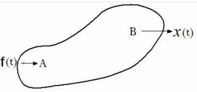
(11) vibrational modes’ series. This model has been known as a Modal model. This model is in a form of natural frequencies with their damping coefficients and vibrational mode shapes. Knowing of this point is important because this model always introduces free vibration without any extrinsic force or excitation and the output is natural modes of a structure. The third step is dedicated to consider structure response in which Frequency Response Function (FRF) or Impulse Response Function (IRF) is calculated. 2.2.2. Experimental track of a vibrational analysis. Prior to start investigating of experimental track of a vibrational analysis, Frequency Response Function is explained. In the Modal test, the body is vibrated in a point and the response is taken out from the other point (Figure 2.2.2.1).. Figure 2.2.2.1- Exemplary body under excitation at point “A” If the body is assumed linear (this assumption is usually a good assumption under condition that the amplitude of vibration is low) and the amplitude ratio of vibration at point “B” to excitation amplitude at point “A”, does not related to intensity and excitation type at point “A” and it is always constant. If the excitation at point “A” is a sinusoidal function, the response is a sinusoidal function at “B” and amplitude ratio 𝑋0 at “B” to amplitude 𝐹0 at “A” is always constant and it does not depend on 𝐹0 (Figure 2.2.2.2).. 9.

(12) 𝑋0 𝐹0. = 𝐶𝑡𝑒. (1.1.2.1). Figure 2.2.2.2- Body excitation and response with its functions If the excitation frequency at point “A” , which is 𝜔, is changed, the ratio 𝑋 of 𝐹0 will be changed. This ratio reaches to its maximum amount when 0. excitation frequency coincides with natural frequencies of the body. This 𝑋 coincidence is named resonance. If different values of the ratio 0 is plotted 𝐹0. versus , a figure will be obtained which is similar to figure (2.2.2.3).. Figure 2.2.2.3- Frequency Response Functions (FRFs). 10.

(13) This figure is named Frequency Response Function. The place of maximum points of this function (𝜔1 , 𝜔2 , 𝜔3 ) is named natural frequency.. In figure (2.2.2.3), H is an estimator which is obtained from following relations:. 𝐻1 (𝜔) =. 𝑆𝑓𝑥 (𝜔). (2.2.2.1). 𝑆. (2.2.2.2). 𝑆𝑓𝑓 (𝜔). (𝜔). 𝐻2 (𝜔) = 𝑆𝑥𝑥 (𝜔) 𝑥𝑓. In which 𝑆𝑥𝑥 and 𝑆𝑓𝑓 are Auto Spectrum density of x and f parameters, respectively. 𝑆𝑓𝑥 and 𝑆𝑥𝑓 are Cross Spectrum density of x , f and f , x , respectively. It is usually demonstrated the ratio. Decibel (dB). This quantity is defined as follows:. 𝑑𝐵 = 20. log10 𝑥. 𝑋0 𝐹0. corresponding to (2.2.2.3). Frequency is also described corresponding to Hertz (Hz) which has a 𝑟𝑎𝑑 relation with 𝜔 ( 𝑠𝑒𝑐 ) as follows: 𝜔. 𝑓 = 2𝜋. (2.2.2.4). Response model consists of a series of Frequency Response Functions (FRFs) that should be defined over a frequency interval. Therefore, it should be noted to three steps and models of spatial, Modal and response. As it has been shown in figure (2.2.1.1), it is possible to follow from spatial model to frequency response analysis. This track is actually named Experimental Modal Analysis which has been shown in following figure. Experimental Modal Analysis Response. Vibration. Structural. Properties. Modes. Model. Figure 2.2.2.4- Experimental Modal Analysis track. 11.

(14) 2.3 Research methods In this thesis, OMA technique based on transmissibility measurements will be applied. First a two-DOF mechanical system will be studied in order to investigate the applicability of the output-only identification technique using transmissibility measurements. This will be followed by a simulation using a beam system. Finally, a vibration experiments will be conducted on a cantilever beam. A combination of transmissibility approach and Experimental Modal Analysis is used to extract resonance frequencies, modal vectors and damping ratios. Combination of transmissibility approach and Experimental Modal Analysis is used to extract modal parameter inclusive of resonance frequencies, modal vectors and damping ratios. MATLAB software is dominantly used in this thesis. Therefore, in this thesis, modal parameters for a structure subject to a moving load have been calculated by means of transmissibility measurement. Herein Finite Element Model for a clamped-clamped beam has been taken into account in ABAQUS.. 3 Operational Modal Analysis Operational Modal Analysis uses structural response measurements from ambient excitation to extract modal characteristics. Thus, it is also called ambient, natural-excitation or output-only modal analysis. In Experimental Modal Analysis (EMA), forces acting on a structure are recorded and the response resulting from any unmeasured force is regarded as unwanted noise that needs to be removed. In the case of Operational Modal Analysis for in situ measurements, the response of the structure to the unmeasured operational loading is recorded and the modal parameters are extracted from the out-put only data by means of assumptions on the nature of the unknown forces.. 12.

(15) Operational Modal Analysis is a complementary technique to traditional modal analysis methods and is based upon measuring only the response of test structures. The technique enables the testing of structures such as running cars, vehicle-bridge interaction, airplanes, etc., that are impossible or difficult to excite by external forces, owning to boundary condition or physical size. The technique presented in this thesis is a Singular Value Decomposition (SVD) technique. The classical approach presents reasonable estimations of natural frequencies and mode shapes if the modes are well separated. However, in the case of close modes, it can be difficult to detect the close modes and even in the case of where close mode are detected, estimation becomes heavily biased. Further, the frequency estimations are limited by the frequency resolution of the spectral density estimations and in all cases damping estimation is uncertain or impossible. In the Frequency Domain Decomposition (FDD) identification, the first step is to estimate the transmissibility matrix. The estimate of the transmissibility is then decomposed by taking the Singular Value Decomposition (SVD) of the matrix [2]. 𝑇𝑅𝑖𝑗 = 𝑈𝑖 𝑆𝑖 𝑉𝑖. Where the matrix 𝑈𝑖 is a unitary matrix holding the singular vectors 𝑢𝑖𝑗 and 𝑆𝑖 is a diagonal matrix holding the scalar singular values 𝑠𝑖𝑗 . Near a peak corresponding to the k th mode in the spectrum this mode or may be a possible close mode will be dominating We can point out that OMA has many advantages such as OMA is cheap and fast to conduct. We don’t need elaborate excitation equipment and boundary condition simulation which results in reducing response measurement comparing to traditional modal testing. We can obtain the dynamic characteristic of the complete system at much more representative working points as well. Moreover, the model characteristics under real loading are experienced and all or part of measurement coordinates can be used as references. The closed-spaced or even repeated modes can easily be handled and the results are suitable for real world complex structures. In addition, Operational modal identification with output-only measurements can be utilized not only for dynamic design, structural control, but vibration-based health monitoring and damage detection of the structure [3].. 13.

(16) One limiting constraint of the current OMA techniques is that the nonmeasured excitations to the system in operation must be white-noise sequences. In practice however, structural vibrations observed in operation cannot always be considered as pure white-noise excitation [3]. In this thesis OMA technique based on transmissibility measurements will be applied. This method does not make any assumption about the nature of forces and reduces the risk of wrongly identifying the modal parameters due to the presence of non-white-noise sequence. In this contribution, first a two-DOF mechanical system was studied in order to investigate of applicability of the output-only identification technique using transmissibility measurements. Subsequently, numerical vibration experiments were conducted on a cantilever beam in order to study of modal parameters for a lumped mechanical system using transmissibility measurements.. 4 Transmissibility concept In the scope of system identification, most identification algorithms are either based on input and output time-history measurements or frequency domain identification algorithms from the input and output spectra. In the case of a typical modal analysis experiment, a large amount of data is available and some preprocessing of the data is recommended to reduce both the size of the data set and noise levels before starting the parametric identification of the model parameters [3]. In EMA applications it is common to reduce the amount of data and the noise levels by using the Frequency Response Functions (FRFs) as primary data instead of the input and output spectra. The measured forces and vibration responses are divided into different data blocks in order to average and estimate the FRFs [3]. In some applications, e.g. civil engineering one is more interested in obtaining modal models from structures during their operational conditions to model the interaction between the structure and its environment. Another advantage of an in-operation modal analysis is that nonlinear effects are linearized around the operational working point. For these applications force excitation are difficult or even impossible to measure. On the other. 14.

(17) hand, elimination of this excitation is often impossible so one only way is to measure vibration responses [3]. From this output data only in order to estimate modal parameters from these responses only is referred to as stochastic system identification or more specific Operational Modal Analysis (OMA). In the field of stochastic system identification one can generally divide the identification techniques into two basic subcategories: -. Data-driven stochastic identification algorithms which directly start the identification from the output time sequences or output spectra. Correlation or auto-and cross-spectral-density driven stochastic identification algorithms which estimate in a first step the covariance or auto- and cross-spectral densities between the outputs and certain reference sensors [3].. In the field of transmissibilities identification attention will be paid to the use of transmissibilities as a primary data to derive modal parameters. No assumption about the nature of force is made and transmissibilities are obtained by taking the ratio of two response spectra, i.e. Tij = Xi (s)/Xj (s).. In general, it is not possible to identify modal parameters from transmissibility measurements by assuming a single force that is located in DOF k. Consequently, the poles of the transmissibility function equal the zeros of transfer function. In general, the peaks in the magnitude of a transmissibility function do not at all coincide with the resonances of the system. It will be shown transmissibility is independent from the location of the input DOF k of the unknown force at resonance frequencies. This is directly the result of the fact that transmissibilities vary with the location of the applied forces, but become independent of them at the system’s poles and all converge to the same unique value.. 5 Simulation study A simulation study is carried out using a 2-DOF system as well as a cantilever beam system. Modal parameters for both systems are found. 15.

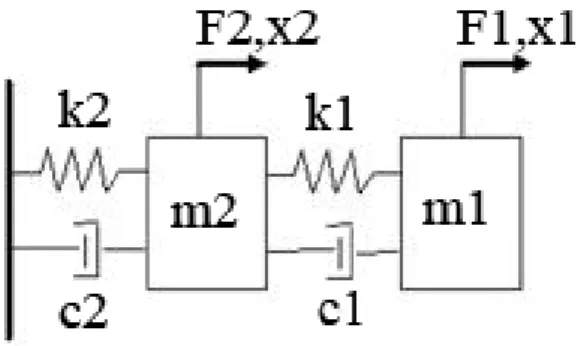
(18) through OMA techniques in which transmissibility measurement is the most dominant technique to obtain modal parameters. MATLAB software is utilized to perform simulations. For the 2-DOF system, a random force is applied to DOF 1 while responses are calculated at DOF1 and DOF 2. A force is then applied to DOF2 and responses are calculated at both DOFs. For the beam case we assume an Euler-Bernoulli cantilever beam and the modal parameters for the first five modes are studied. Five points are considered along the beam and a random force is used as an input to the system at all points while responses are calculated at all points.. 5.1 2-DOF system Figure 5.1.1 shows a simple example of a two-DOF system. We only assume that we know X1 (s) and X2 (s). Now we want to find residues Apqr and the poles 𝜆𝑟 . We will first start with system equations:. Figure5.1.1- A two-DOF system The time-domain model is given by �. m1 0. c 0 ẍ 1 �� + � 1 m2 ẍ 2 -c1. -c1 k ẋ � � 1� + � 1 c1 + c2 ẋ 2 -k1. A Laplace-domain model can be written as:. 16. x1 -k1 F � �x � = � 1 � F2 2 k1 + k 2. (5.1.1).

(19) �. H11 (s) H12 (s) F1 (s) X (s) �� =� 1 � H21 (s) H22 (s) F2 (s) X2 (s). (5.1.2). The transfer functions in Eq. (5.1.2) can be written with modal parameters as: A∗pqr. Apqr. Hpq (s) = ∑N r=1 𝑠−𝜆 + 𝑠−𝜆∗ 𝑟. (5.1.3). 𝑟. For example, H11 (s) can be written as: A. A∗. A. A∗. 111 112 111 112 H11 (s) = 𝑠−𝜆 + 𝑠−𝜆 ∗ + 𝑠−𝜆 + 𝑠−𝜆∗ 1. 1. 2. 2. (5.1.4). Assume that we have two measurements, A and B: Case A: Only force in DOF 1. Case B: Only force in DOF 2. For Case A we get (see Eq. (5.1.2)): �. H11 H21. �. H11 H21. Xa H12 F1a � � � = � 1a � H22 0 X2. (5.1.5). For Case B we get (see Eq. (5.1.2)): Xb H12 0 � � b � = � 1b � H22 F2 X2. (5.1.6). We can now define two transmissibility functions as: Xa. H. Xb. H. a T12 = X1a = H11 2. (5.1.7). 21. b T12 = X1b = H12 2. (5.1.8). 22. Hence, Ta12 is the transmissibility for case A, while Tb12 is the transmissibility for case B. The relationship between the transmissibilities and the FRFs is obtained directly from Eq. (5.1.5)-(5.1.6). In general Ta12 ≠ Tb12 , since these functions depend on the location of the force as can be seen in Eq. (5.1.7)-(5.1.8). However, as will be shown next, the two functions are identical at the system poles. We start with Ta12 . By using the modal model in Eq. (5.1.3), we can rewrite Eq. (5.1.7) as. 17.

(20) a T12. =. ∗. A A ∑2r=1 11r+ 11r∗ 𝑠−𝜆𝑟 𝑠−𝜆𝑟 A∗ A 2 ∑r=1 21r+ 21r∗ 𝑠−𝜆𝑟 𝑠−𝜆𝑟. (5.1.9). We will now study what happens if ‘s’ is close to the first pole. The nominator and the denominator of Eq. (5.1.9) is multiplied with (𝑠 − 𝜆1 ) and the following limit is studied: lims→𝜆1 �. (𝑠−𝜆1 )A111 (𝑠−𝜆1 )A∗111 (𝑠−𝜆1 )A112 (𝑠−𝜆1 )A∗112 + + + ∗ 𝑠−𝜆1 𝑠−𝜆2 𝑠−𝜆∗1 𝑠−𝜆2 ∗ (𝑠−𝜆1 )A211 (𝑠−𝜆1 )A211 (𝑠−𝜆1 )A212 (𝑠−𝜆1 )A∗212 + + + ∗ 𝑠−𝜆1 𝑠−𝜆2 𝑠−𝜆∗1 𝑠−𝜆2. �. (5.1.10). It is seen in Eq. (5.1.10) that many terms will be zero as s → 𝜆1 . We will then get: (𝑠−𝜆1 )A111 𝑠−𝜆1 (𝑠−𝜆1 )A211 𝑠−𝜆1. lims→𝜆1 �. �=. (𝑠−𝜆1 )A111 � 𝑠−𝜆1 (𝑠−𝜆1 )A211 � lims→𝜆1 � 𝑠−𝜆1. lims→𝜆1 �. A. = A111. (5.1.11). 211. Next, we study what happens to Tb12 if ′s′ is close the first pole. By using the modal model in Eq. (5.1.3), we can rewrite Eq. (5.1.8) as b T12 =. ∗. A A ∑2r=1 12r+ 12r∗ 𝑠−𝜆𝑟 𝑠−𝜆𝑟 A∗ A 2 ∑r=1 22r+ 22r∗ 𝑠−𝜆𝑟 𝑠−𝜆𝑟. (5.1.12). Expanding Eq. (5.1.12) and multiplying with (𝑠 − 𝜆1 ) gives: lims→𝜆1 �. (𝑠−𝜆1 )A121 (𝑠−𝜆1 )A∗121 (𝑠−𝜆1 )A122 (𝑠−𝜆1 )A∗122 + + + ∗ 𝑠−𝜆1 𝑠−𝜆2 𝑠−𝜆∗1 𝑠−𝜆2 ∗ ∗ (𝑠−𝜆 )A (𝑠−𝜆 )A (𝑠−𝜆1 )A221 1 221 (𝑠−𝜆1 )A222 1 222 + + + ∗ 𝑠−𝜆1 𝑠−𝜆2 𝑠−𝜆∗1 𝑠−𝜆2. It then follows that: (𝑠−𝜆1 )A121 𝑠−𝜆1 (𝑠−𝜆1 )A221 𝑠−𝜆1. lims→𝜆1 �. �=. (𝑠−𝜆1 )A121 � 𝑠−𝜆1 (𝑠−𝜆1 )A221 � lims→𝜆1 � 𝑠−𝜆1. lims→𝜆1 �. A. = A121 221. �. In summary, we have the following relationship at the first pole, λ1 A. a (𝑠) T12 = A111 ,. Likewise:. A. 211. b (s) T12 = A121 , 221. (5.1.13). (5.1.14). 𝑖𝑓 𝑠 = λ1. (5.1.15). 𝑖𝑓 𝑠 = λ1. (5.1.16). The residues are related to each other according to the following relationship (r is the mode number):. 18.

(21) Apqr =. Apkr ⋅Aqkr. (5.1.17). Akkr. We can now rewrite Eq. (5.1.16). From Eq. (5.1.17) we get that: A121 =. A221 =. A111 ⋅A211 A111. A211 ⋅A211 A111. , (𝑝 = 1, 𝑞 = 2, 𝑘 = 1). , (𝑝 = 2, 𝑞 = 2, 𝑘 = 1). (5.1.18) (5.1.19). Insertion of Eq. (5.1.18)-(5.1.19) in Eq. (5.1.16) yields: b (s) T12 =. A ⋅A � 111 211 � A111. A ⋅A � 211 211 � A111. A. ⋅A. A. = A111 ⋅A211 = A111 211. 211. 211. Hence, Ta12 (𝑠) and Tb12 (𝑠) takes the same value at 𝑠 = λ1. A. a (𝑠) b (𝑠) T12 = T12 = A111 , 211. 𝑖𝑓 𝑠 = λ1. (5.1.20). (5.1.21). Using the same way of reasoning (Eq. (5.1.10)-(5.1.21)) but for the second pole, 𝑠 = λ2, we can show that the following relationship holds: A a (𝑠) b (𝑠) T12 = T12 = A112 , 𝑖𝑓 𝑠 = λ2 (5.1.22) 212. Hence, the transmissibilities will cross each other at resonance frequencies.. In order to extract resonance frequencies with a higher precision we introduce Singular Value Decomposition (SVD) for the transmissibility matrix. We will obtain three distinct matrices after decomposition. We create transmissibility matrix as follows: 1. 2. (5.1.23) 𝑇𝑅 = �𝑇21 𝑇21 � 1 1 The proposed matrix is of rank 2 but in case of resonance frequencies transmissibilities are equal to each other so the proposed matrix is of rank one. In this case, the diagonal components of the second decomposed matrix (naming S matrix) are close to zero except for component S(1,1). Therefore, if we plot the inverse component S(2,2) versus frequency, for example, the peaks of this plot reveal resonance frequencies. This is demonstrated in Figure 5.1.2.2. In order to find modal damping we use Receptance and “ 3dB-bandwith” method in accordance with formula ( 5.1.24) [4]:. 19.

(22) 𝐵𝑟 = 𝑓𝑢 − 𝑓𝑙 𝐵. 𝜁 ≈ 2𝑓𝑟. (5.1.24). 𝑑. Where 𝑓𝑢 and 𝑓𝑙 are the upper and lower frequencies which are defined so that the power (amplitude square) of |𝐻(𝑓)| has been halved in relation to the peak value of approximately �𝐻(𝑓𝑑 )�. Moreover, 𝑓𝑑 is a damped natural frequency. Therefore we can easily find modal damping in accordance with figure (5.1.2.4). Un-scaled modal vectors can be determined by using relations (5.1.21) and (5.1.22). If we make the following assumption: A111 = 1. A112 = 1. (mode 1) (mode 2). We will then obtain the modal vectors as: ψ1 = �1. ψ2 = �1. 1. Ta12 (𝑠=λ1 ). �. (5.1.25). 1 � = λ2 ). a (𝑠 T12. To find scaled mode shape please see Refs [5-6]. An example is illustrated next using the following mass, damping and stiffness: 𝑚1 = 75 𝐾𝑔, 𝑚2 = 125 𝐾𝑔, 𝑐1 = 150 𝑁. 𝑠�𝑚 , 𝑐2 = 90 𝑁. 𝑠�𝑚 , 𝑘1 = 400 𝐾𝑁�𝑚 , 𝑘2 = 200 𝐾𝑁�𝑚. The calculated transmissibilities are illustrated in Fig. 5.1.2.. 20.

(23) Figure5.1.2-Calculated transmissibility for a two-DOF mechanical system. Figure5.1.3- Inverse S(2,2) versus frequency. 21.

(24) As we can see the result from figure 5.1.2 and 5.1.3 at the second resonance frequency is different with each other but figure 5.1.2.2 shows the precise value. Thus: 𝑓1 = 4.834[𝐻𝑧]. 𝑓2 = 15.23[𝐻𝑧] The modal damping is obtained as follows: 𝐵. 𝜁1 ≈ 2𝑓𝑟 = 𝜁2 ≈. 𝑑. 4.88−4.807 2×4.843. = 0.007536. 𝐵𝑟 15.56 − 15 = = 0.018348 2 × 15.26 2𝑓𝑑. According to relation (5.1.25), the modal vectors are given by: ψ1 = �1. ψ2 = �1. 1. Ta12 (𝑠=λ1 ). � = �1. 1. 1.21. � = [1 0.8264 ]. 1 1 � = �1 � = [1 −0.7241 ] = λ2 ) −1.381. a (𝑠 T12. Figure5.1.4- Error at resonance frequencies. 22.

(25) 5.1.1. Conclusion. As it was seen, the result from transmissibility measurement for the simplest system, a 2-DOF system, was acceptable. If we look through figure 5.1.2.4, we will find out the resonance frequencies from transmissibility are close to calculated flexibility. In following, we will extend the degree of freedom to a MDOF system such as a beam to investigate if the transmissibility is applicable for all system or not.. Figure5.1.5- Calculated flexibility for the studied 2-DOF system. 5.2 Beam system The OMA method applied in previous section is next demonstrated on a cantilever beam system. The theoretical modal parameters for a continuous beam system are first derived. For a prismatic beam with constant mass distribution and crosssectional bending stiffness, the following relationship holds:. 23.

(26) 𝑑4 𝑌(𝑥) 𝑑𝑥 4. 𝑑4 𝑌(𝑥) 𝑑𝑥 4. −. 𝜔2𝑚 𝐸𝐼. 𝑌(𝑥) = 0. (5.2.1). − 𝛽 4 𝑌(𝑥) = 0. 𝛽4 =. 𝜔2 𝑚. (5.2.2). 𝐸𝐼. The following boundary conditions are introduced: 𝑌 ′ (0) = 0. 𝑌(0) = 0. 𝑌 ′′ (𝐿) = 0. 𝑌 ′′′ (𝐿) = 0. Expanding Eq. (5.2.2), we get:. 𝑌(𝑥) = 𝐴 sin 𝛽𝑥 + 𝐵 cos 𝛽𝑥 + 𝐶 sinh 𝛽𝑥 + 𝐷 cosh 𝛽𝑥. 𝑌 ′ (𝑥) = 𝐴𝛽 cos 𝛽𝑥 − 𝐵𝛽 sin 𝛽𝑥 + 𝐶𝛽 cosh 𝛽𝑥 + 𝐷𝛽 sinh 𝛽𝑥. (5.2.3) (5.2.4) (5.2.5). 𝑌 ′′ (𝑥) = −𝐴𝛽 2 sin 𝛽𝑥 − 𝐵𝛽 2 cos 𝛽𝑥 + 𝐶𝛽 2 sinh 𝛽𝑥 + 𝐷𝛽 2 cosh 𝛽𝑥. (5.2.6). 𝑌 ′′′ (𝑥) = −𝐴𝛽 3 cos 𝛽𝑥 + 𝐵𝛽 3 sin 𝛽𝑥 + 𝐶𝛽 3 cosh 𝛽𝑥 + 𝐷𝛽 3 sinh 𝛽𝑥. (5.2.7). Considering 𝛽 ≠ 0, yields the following system of equations: 0 1 � − sin 𝛽𝐿 − cos 𝛽𝐿. 1 0 − cos 𝛽𝐿 sin 𝛽𝐿. 0 1 sinh 𝛽𝐿 cosh 𝛽𝐿. 1 𝐴 0 𝐵 �� = 0 cosh 𝛽𝐿 𝐶 sinh 𝛽𝐿 𝐷. (5.2.8). The non-Trivial solution is obtained by taking the determinant as: 0 1 𝑑𝑒𝑡 � − sin 𝛽𝐿 − cos 𝛽𝐿. 1 0 − cos 𝛽𝐿 sin 𝛽𝐿. ∴ 1 + cos 𝛽𝐿 cosh 𝛽𝐿 = 0. 0 1 sinh 𝛽𝐿 cosh 𝛽𝐿. 1 0 �=0 cosh 𝛽𝐿 sinh 𝛽𝐿. (5.2.9). (5.2.10). It then follows that the natural frequencies can be written as: 𝐸𝐼. 𝜔 = 𝛽2�𝑚. (5.2.11). and the first four eigenvalues are given by. 24.

(27) 𝛽1 𝐿 1.8751 𝛽2 𝐿 4.6941 � �=� � 𝛽3 𝐿 7.8548 𝛽4 𝐿 10.996. (5.2.12). For the subsequent simulation, the following parameters are used: The length of the beam is set to L=0.75m and the width and height of the beam are W = 14 × 10−3 𝑚 , 𝐻 = 6 × 10−3 𝑚 , respectively.. The beam material is steel with 𝑑 = 7850 equal to 𝐸 = 200 𝐺𝑃𝑎.. 𝐾𝑔. 𝑚3. and Elasticity modulus is. With these parameters, the first natural frequency is 𝑓0 = 8.6974 [𝐻𝑧] as given by Eq. (5.2.12).For the numerical simulation, six points along the beam are selected as response DOFs We excite the beam with a random force at one DOF at the time. In each step, the responses at all DOFs are determined. The process is repeated for all six DOFs. We assume a random force with length 𝑛 = 256 × 1024 and we use a lowpass filter. Number of Fast Fourier Transform 𝑁𝐹𝐹𝑇 = 16184 and the sampling frequency is 𝑓𝑠 = 10000 𝐻𝑧. We take the first five modes into account. Estimated transmissibility functions are illustrated in Fig. 5.2.1 to Fig. 5.2.4.. 25.

(28) Figure5.2.1- Transmissibility measurement (𝑇21 ) at all DOFs excitement. Figure5.2.2- Transmissibility measurement (𝑇31 ) at all DOFs excitement. 26.

(29) Figure5.2.3- Transmissibility measurement (𝑇41 ) at all DOFs excitement. Figure5.2.4- Transmissibility measurement (𝑇51 ) at all DOFs excitement The result is summarized in table 5.2.1.. 27.

(30) Transmissibil ity 𝑇21 𝑇31 𝑇41 𝑇51. Resonan ce 1 8.651 8.651 8.651 8.651. Resonan ce 2 54.37 54.37 54.37 54.37. Table 5.2.1: Comparison transmissibilities. between. Resonan ce 3 152.6 152.6 152.6 152.6 the. Resonan ce 4 299.1 299.1 299.1 299.1. results. from. Resonan ce 5 494.3 494.3 494.3 494.3 different. A Singular Value Decomposition (SVD) of the transmissibility matrix is carried out next. We create transmissibility matrix as: 𝑇1 ⎡ 21 1 ⎢𝑇31 1 𝑇𝑅 = ⎢𝑇41 ⎢ 1 ⎢𝑇51 ⎣1. 2 𝑇21 2 𝑇31 2 𝑇41 2 𝑇51 1. 3 𝑇21 3 𝑇31 3 𝑇41 3 𝑇51 1. 4 𝑇21 4 𝑇31 4 𝑇41 4 𝑇51 1. 5 𝑇21 ⎤ 5 𝑇31 ⎥ 5⎥ 𝑇41 ⎥ 5 𝑇51 ⎥ 1⎦. (5.2.13). The proposed matrix is of rank 5 but in case of resonance frequencies transmissibilities are equal to each other so the proposed matrix is of rank one. In this case, the diagonal component of the second decomposed matrix (naming S matrix) are close to zero except for component S(1,1). Therefore, by studying the inverse component S(2,2) versus frequency, for example, the peaks reveal resonance frequencies. This is illustrated in Figure 5.2.5.. 28.

(31) Figure5.2.5- Inverse S(2,2) versus frequency As seen in Fig. 5.2.5, the resonance frequencies are: 𝑓1 = 8.651[𝐻𝑧] 𝑓2 = 54.37[𝐻𝑧]. 𝑓3 = 152.6[𝐻𝑧] 𝑓4 = 299.1[𝐻𝑧] 𝑓5 = 494.3[𝐻𝑧] After finding resonance frequencies we should find unscaled modal shapes. To do so, we consider the transmissibility matrix (5.2.13) at resonance frequencies. First, the theoretical mode shapes are determined for the studied system. We have all residues and damping ratios so we can find modal vector. To do so we assume j=5 (DOF at input) and different output measurements for i=1,2,3,4,5 (DOF at output). Therefore, we will take out all residues for DOF j=5 and different output measurements at all resonance frequencies.. 29.

(32) 𝐴1 represents all of residues 𝐴𝑖51 for i=1,2,…,5 at the first resonance.. MATLAB function "cantilever" has been used to find residues. Please see appendix A1.. i=1. 𝑨𝟏. 0-0.0047i. 𝑨𝟐. 0+0.0036i. 𝑨𝟑. 0-0.0025i. 𝑨𝟒. 0+0.0016i. 0-0.0009i. i=2. 0-0.0170i. 0+0.0081i. 0-0.0022i. 0-0.0007i. 0+0.0009i. i=3. 0-0.0341i. 0+0.0070i. 0+0.0020i. 0-0.0007i. 0-0.0009i. i=4. 0-0.0537i. 0-0.0008i. 0+0.0017i. 0+0.0014i. 0+0.0008i. i=5. 0-0.0740i. 0-0.0118i. 0-0.0042i. 0-0.0022i. 0-0.0013i. Table 5.2. 2: Resultant residues for the cantilever beam Now we will find Q-factors in order to find modal vectors: 𝑄1 =. 1 = 𝑗4𝜋𝑓𝑑1. 0 - 0.0091986i 𝑄2 =. 1 = 𝑗4𝜋𝑓𝑑2. 𝑄3 =. 1 = 𝑗4𝜋𝑓𝑑3. 0 - 0.0014636i. 0 - 0.0005215i 𝑄4 =. 1 = 𝑗4𝜋𝑓𝑑4. 0 - 0.0002661i 𝑄5 =. 1 = 𝑗4𝜋𝑓𝑑5 30. 𝑨𝟓.

(33) 0 - 0.0001609i Using the equation 𝜓1𝑛 𝜓5𝑛 𝐴15𝑛 ⎧𝜓 𝜓 ⎫ ⎧𝐴 ⎫ ⎪ 25𝑛 ⎪ ⎪ 2𝑛 5𝑛 ⎪ 𝐴 𝐴35𝑛 = 𝑄𝑛 𝜓3𝑛 𝜓5𝑛 , 𝑛ℇ{1,2,3,4,5} => 𝜓5𝑛 𝜓5𝑛 = 55𝑛 => 𝜓5𝑛 = 𝑄𝑛 ⎨𝐴45𝑛 ⎬ ⎨𝜓 𝜓 ⎬ ⎪ ⎪ ⎪ 4𝑛 5𝑛 ⎪ ⎩𝐴55𝑛 ⎭ ⎩𝜓5𝑛 𝜓5𝑛 ⎭. �. 𝐴55𝑛 𝑄𝑛. (5.2.14). Thus 𝜓1𝑛 𝐴15𝑛 ⎧𝜓 ⎫ ⎧𝐴 ⎫ ⎪ 2𝑛 ⎪ ⎪ 25𝑛 ⎪ 1 𝐴35𝑛 {𝜓}𝑛 = 𝜓3𝑛 = ⎨ ⎬ ⎨𝜓4𝑛 ⎬ 𝑄𝑛�𝐴𝑄55𝑛 𝑛 ⎪𝐴45𝑛 ⎪ ⎪ ⎪ ⎩𝐴55𝑛 ⎭ ⎩𝜓5𝑛 ⎭. (5.2.15). We can then obtain the modal vectors as: 𝐴551 −0.0740i 𝜓51 = � = � = 2.8361 𝑄1 − 0.0092i. 𝐴552 −0.0118i = � = 2.8429 𝜓52 = � 𝑄2 − 0.00146i. 𝐴553 −0.0042i 𝜓53 = � = � = 2.8379 𝑄3 − 0.0005215i 𝐴554 −0.0022i 𝜓54 = � = � = 2.8753 𝑄4 − 0.0002661i. 31.

(34) 𝐴555 −0.0013i 𝜓55 = � = � = 2.8416 𝑄5 − 0.00016099i mode1=A1/(𝜓51 *Q1) mode2=A2/(𝜓52 *Q2) mode3=A3/(𝜓53 *Q3) mode4=A4/(𝜓54 *Q4). Mode5=A5/(𝜓55 *Q5) Mode 1. Mode 2. Mode 3. Mode 4. Mode 5. i=1. 0.1816. -0.8562. 1.7192. -2.1438. 1.8760. i=2. 0.6538. -1.9438. 1.4957. 0.8974. -1.9810. i=3. 1.3115. -1.6765. -1.3474. 0.9285. 1.9915. i=4. 2.0632. 0.1992. -1.1230. -1.8288. -1.7077. i=5. 2.8440. 2.8440. 2.8440. 2.8440. 2.8440. Table 5.2. 3: Resultant mode shapes for the cantilever beam Therefore, the theoretical mode shapes are:. 32.

(35) 0 0 ⎡0.1816⎤ ⎡−0.8562⎤ ⎢ ⎥ ⎢ ⎥ 0.6538⎥ −1.9438⎥ ⎢ ⎢ 𝜓1 = 𝜓2 = ⎢1.3115⎥ ⎢−1.6765⎥ ⎢2.0632⎥ ⎢ 0.1992 ⎥ ⎣2.8440⎦ ⎣ 2.8440 ⎦ 0 ⎡ 1.8760 ⎤ ⎢ ⎥ −1.9810⎥ ⎢ 𝜓5 = ⎢ 1.9915 ⎥ ⎢−1.7077⎥ ⎣ 2.8440 ⎦. 0 ⎡ 1.7192 ⎤ ⎢ ⎥ 1.4957 ⎥ ⎢ 𝜓3 = ⎢−1.3474⎥ ⎢−1.1230⎥ ⎣ 2.8440 ⎦. 0 ⎡−2.1438⎤ ⎢ ⎥ 0.8974 ⎥ ⎢ 𝜓4 = ⎢ 0.9285 ⎥ ⎢−1.8288⎥ ⎣ 2.8440 ⎦. Figure5.2.6- Theoretical mode shapes for the studied cantilever beam. Note that only six response points are used to describe the shape. Now, we want to find mode shapes by the OMA method, that is, from the transmissibility functions. According to Eq. (5.1.15) and Eq. (5.2.14), we can conclude that A. 1 (𝑠) T21 = A211 A. 111. 𝑖𝑓 𝑠 = λ1 𝑄 𝜓. 𝜓. 𝜓. 1 (𝑠) T21 = A211 = 𝑄1 𝜓21𝜓11 = 𝜓21 111. 1. 11. 11. (5.2.16). 11. 33.

(36) With the same manner, we will have: 1 (𝑠) = T31. 𝜓31 , 𝜓11. 1 (𝑠) T41 =. 𝜓41 , 𝜓11. 1 (𝑠) T51 =. 𝜓51 𝜓11. If we assume 𝜓11 = 1, we can then find all of mode shapes. The result can be seen in Fig. 5.2.7. .. Figure5.2.7- Mode shapes for cantilever beam by OMA method In order to verify that the mode shapes are identical, a MAC matrix is calculated for the two set of modal vectors, as shown in Fig. 5.2.8 In addition, a FEM-based model is created in ABAQUS and the first five modes are visualized in Fig. 5.2.9 to Fig. 5.2.13.. 34.

(37) Figure 5.2.8MAC matrix. Figure5.2.9- The first mode shape for cantilever beam By ABAQUS. 35.

(38) Figure5.2.10- The second mode shape for cantilever beam By ABAQUS. Figure5.2.11- The third mode shape for cantilever beam By ABAQUS. 36.

(39) Figure5.2.12- The fourth mode shape for cantilever beam By ABAQUS. Figure5.2.13- The fifth mode shape for cantilever beam By ABAQUS. 5.2.1. Conclusion. As it was seen in this section, extension degree of freedom of the system from a 2-DOF system to a MDOF system did not disrupt through transmissibility method. In following, we are going to validate this simulation by means of an experiment by transmissibility method.. 37.

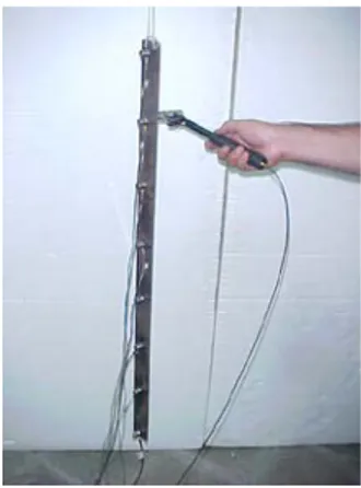
(40) 6 Experimental validation An experimental test for verification and validation of the OMA method based on transmissibility functions is presented in this chapter. We assumed a beam with free-free end as it has been shown in figure 6.1.. . Figure 6.1- A beam with a free-free end boundary condition. The properties of this beam are as follows: Length(L=1000 mm), thickness(t=6.48 mm), height(H=49.3 mm), mass(m=2.3 Kg), Young’s modulus(E=1.845e11), Poisson’s Ratio(υ=0.3). Eight accelerometers are placed along the beam and an impulse hammer is used to excite the structure. Test data is analysed and saved by means of Pulse Software for Modal Analysis. Modal parameters are identified from estimated transmissibility functions, according to section 5.2, matrix 5.2.23 and the SVD method. The rank of the transmissibility matrix is eight but at the resonance frequencies the matrix rank will be one. Due to the existence of noise in the data, the following formula is utilized to estimate transmissibility functions: 𝑋 (𝑠). 𝑋 (𝑠)×𝑋 (𝑠)∗. 𝑇𝑖𝑗 = 𝑋 𝑖 (𝑠) = 𝑋 𝑖 (𝑠)×𝑋𝑖 (𝑠)∗ = 𝑗. 𝑗. 𝑖. 𝑃𝑆𝐷(𝑋𝑖 (𝑠)). (6.1). 𝐶𝑆𝐷. 38.

(41) Figure6.2- Inverse S(2,2) versus frequency Figure 6.2 simply shows resonance frequencies by means of singular value decomposition of transmissibility matrix. It is also interesting to compare resonance frequencies resulting from transmissibility with FRFs calculated by using the measured force. Figure 6.3 shows the estimated Frequency Response Functions for this experiment.. 39.

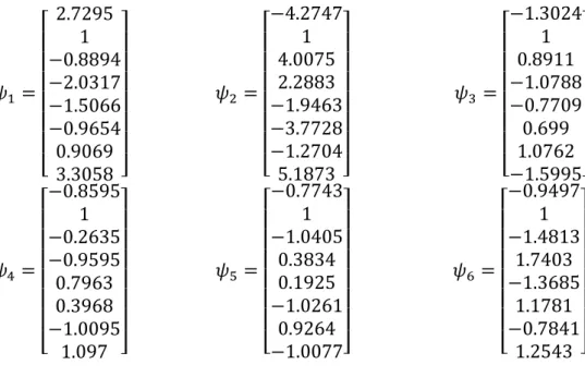
(42) Figure6.3- Frequency Response Function for the experiment Now we are going to find mode shapes by transmissibility measurements. Since there is just one excitation in this experiment so it is not possible to use the relation (5.2.13). Therefore, a little change is made in this relation and the transmissibility matrix is presented as follows:. Τ21 Τ12  Τ31 Τ32 TR =     Τn1 Τn 2 1 1 . Τ13  Τ1n   Τ23  Τ2 n       Τn 3  Τ( n−1) n  1 1 1 . (6.2). Therefore, to find unscaled mode shapes each column of the matrix in relation (6.2) at resonance frequencies shows mode shape ratios so all mode shapes will be easily found in accordance with relation (6.2).. 40.

(43) 2.7295 ⎡ ⎤ 1 ⎢ ⎥ ⎢−0.8894⎥ −2.0317⎥ 𝜓1 = ⎢ ⎢−1.5066⎥ ⎢−0.9654⎥ ⎢ 0.9069 ⎥ ⎣ 3.3058 ⎦ −0.8595 ⎡ ⎤ 1 ⎢ ⎥ −0.2635 ⎢ ⎥ −0.9595⎥ 𝜓4 = ⎢ ⎢ 0.7963 ⎥ ⎢ 0.3968 ⎥ ⎢−1.0095⎥ ⎣ 1.097 ⎦. −4.2747 ⎡ ⎤ 1 ⎢ 4.0075 ⎥ ⎢ ⎥ 2.2883 ⎥ 𝜓2 = ⎢ ⎢−1.9463⎥ ⎢−3.7728⎥ ⎢−1.2704⎥ ⎣ 5.1873 ⎦ −0.7743 ⎡ ⎤ 1 ⎢−1.0405⎥ ⎢ ⎥ 0.3834 ⎥ 𝜓5 = ⎢ ⎢ 0.1925 ⎥ ⎢−1.0261⎥ ⎢ 0.9264 ⎥ ⎣−1.0077⎦. −1.3024 ⎡ ⎤ 1 ⎢ 0.8911 ⎥ ⎢ ⎥ −1.0788⎥ 𝜓3 = ⎢ ⎢−0.7709⎥ ⎢ 0.699 ⎥ ⎢ 1.0762 ⎥ ⎣−1.5995⎦ −0.9497 ⎡ ⎤ 1 ⎢−1.4813⎥ ⎢ ⎥ 1.7403 ⎥ 𝜓6 = ⎢ ⎢−1.3685⎥ ⎢ 1.1781 ⎥ ⎢−0.7841⎥ ⎣ 1.2543 ⎦. Figure 6.4 shows unscaled mode shapes by transmissibility measurements.. Figure6.4- Unscaled mode shapes calculated from transmissibility measurements. Note that only eight points are used to describe the shape.. 41.

(44) As a comparison, the mode shapes calculated from the FRFs are illustrated in figure 6.5.. Figure6.5- Mode shapes obtained from FRFs using classic modal analysis. Note that only eight points are used to describe the shape. In order to verify that the mode shapes are identical, a MAC matrix is calculated as shown in figure 6.6.. 42.

(45) Figure6.6- MAC matrix Moreover, a Finite Element Model of the beam was created using ABAQUS software. The calculated mode shapes are illustrated in Fig. 6.7 to Fig. 6.12.. Figure6.7- The first mode shape for a free-free beam. 43.

(46) Figure6.8- The second mode shape for a free-free beam. Figure6.9- The third mode shape for a free-free beam. Figure6.10- The fourth mode shape for a free-free beam. Figure6.11- The fifth mode shape for a free-free beam. Figure6.12- The sixth mode shape for a free-free beam. 44.

(47) The resonance frequencies obtained from traditional modal analysis based on FRFs, OMA method and ABAQUS model are given in table 6.1. Mode 1. Mode 2. Mode 3. Mode 4. Mode 5 Mode 6. FRFbased Modal Analysis. f=32.09 02 Hz. f=89.01 57 Hz. f=174.50 86 Hz. f=288.140 8 Hz. f=429.9 903 Hz. f=599.7089 Hz. ABAQUS. f=32.74 5 Hz. f=88.72 6 Hz. f=171.53 Hz. f=280.64 Hz. f=416.5 7 Hz. f=579.57 Hz. OMA. f=32 Hz. f=89 Hz. f=174.5 Hz. f=288 Hz. f=430 Hz. f=600 Hz. Table 6.1- Comparison of resonance frequencies between different methods. 6.1 Conclusion This experiment revealed that transmissibility method is still reliable not only in simulation but also in reality. The resultant frequencies in table 6.1 show that Transmissibility method is consistent with traditional method and Finite Element Software such as ABAQUS.. 45.

(48) 7 Harmonic in Transmissibility In previous sections we demonstrated how we can find resonance frequencies by transmissibility measurement but in this section we assert that all peaks which are found by means of Singular Value Decomposition of transmissibility matrix will not always represent resonance frequencies. In this part, we are going through a clamped-clamped beam under a moving load. When any rotating or moving load is applied to a structure, the structure is loaded by a combination of harmonic components and a stochastic background noise that looks more like a coloured white noise loading [7]&[8]. It is important to have some additional tools available for separation of harmonics and structural modes in case of applying output-only modal testing and identification on real cases in which moving load is often in operation during measurements of responses. It should be noted that there are various methods to identify harmonics from structural modes. See Refs [7]&[8]. Now, we are going to represent a simulation of a clamped-clamped beam under moving load. The output responses have been extracted by ABAQUS software. The physical properties of the beam are as follows: Length Young’s modulus Poisson’s ratio Density Cross section Table 7. 1: Beam properties. L=1 m E=15e8 Pa υ=0.3 ρ=7600 𝐾𝑔⁄𝑚3 a=0.08 m & b=0.03m. The beam was divided to twenty parts in order to simulate moving load (Figure 7.1). We also assume a pressure load in a way that after passing every element, the load is moved from previous element to next element so there are twenty load steps.. 46.

(49) Figure 7. 1: Simulation of clamped-clamped beam Then the output data was imported to MATLAB for finding harmonic components and resonance frequencies. The transmissibility matrix was created in accordance with relation (6.2).. Figure 7. 2: Singular Value Decomposition to find resonance frequencies If we look at (Figure 7.2), we can observe a lot of peaks some of which are real resonance frequencies of the system and the others are harmonic components. In order to find real peaks, the dominant peaks were chosen, as they have been shown in (figure 7.2), and they are checked by PULSE software in case of harmonic components. They are known as resonance. 47.

(50) frequencies if they are not harmonic components. Harmonic component lines have been shown in (figure 7.3) by means of PULSE software.. Figure 7. 3: Harmonic components by PULSE software Now the first peak in (figure 7.2) is known as harmonic components and the other peaks are resonance frequencies. Therefore, the first fifth real peaks have been marked in (figure 7.4).. 48.

(51) Figure 7. 4: of resonance frequencies by means of singular value decomposition of transmissibility function In conclusion, we can compare resultant resonance frequencies through both methods in (Table 7.2). We can compare resultant resonance frequencies through both methods in table 7.2. Mode 1 Natural Frequencies by 13.67 transmissibility (Hz) Natural frequencies by 13.63 ABAQUS Software (Hz). 2. 3. 4. 5. 36.13. 71.29. 111.30 166. 37.33. 72.53. 118.55 174.65. Table 7.2: Comparison of resonance frequencies between ABAQUS and transmissibility matrix. 49.

(52) We propose transmissibility relation corresponding mode shape ration in accordance with relation (7.1) to plot all of mode shapes. As it was mentioned before, the first column of this matrix (6.2) shows mode shape ratios at resonance frequencies. Therefore, figure 7.7 shows the resultant mode shapes by means of OMA method.. Τijk =. Α ikn Qn ψ in ψ kn ψ in = = , if s = λn Α jkn Qn ψ jn ψ kn ψ jn. (7.1). Figure 7. 5: Resultant mode shapes by OMA method The resultant mode shapes by ABAQUS have been shown in following.. Figure 7.1: The first mode shape by ABAQUS. 50.

(53) Figure 7.2: The second mode shape by ABAQUS. Figure 7.3: The third mode shape by ABAQUS. Figure 7.4: The fourth mode shape by ABAQUS. Figure 7.5: The fifth mode shape by ABAQUS The resultant mode shapes from MATLAB and ABAQUS have full consistency with each other although we have a little bit difference in value in natural frequencies from different methods. In order to verify correlation between resultant mode shapes by means of OMA method and ABAQUS software MAC criterion is applied which has been shown in (figure 7.13).. 51.

(54) Figure 7.13 Correlation of mode shapes by ABAQUS and OMA using MAC. 8 Conclusion As it was seen through this work, different types of systems have been considered, such as a 2-DOF system and a cantilever beam system to show the robustness of operational modal analysis based on transmissibility measurements. Starting with a 2-DOF system and then increasing the number of DOFs, such as a beam, shows that the method works for arbitrary systems, independently of the number of degrees of freedom of the system. An experimental test was also carried out with promising results. As shown in this work, the method can be used to identify modal parameters without knowing the nature of the actual forces. The unknown operational forces can be arbitrary as long as they are persistently exciting the frequency band of interest. Finally, a case with a moving load was studied with a numerical model. It was shown that the harmonic components generated by the load in the output response could be separated from the actual resonance frequencies, and as a result, the resultant mode shapes from ABAQUS and MATLAB (OMA analysis) were identical to each other.. 52.

(55) 9 Appendices A1. MATLAB function "cantilever" function [poles,residues] = cantilever(m,f0,xin,xout,N,zeta) %CANTILEVER poles and residues for cantilever beam % [poles,residues] = cantilever(m,f0,xin,xout,N,zeta) % poles complex pole column vector in radians % residues complex residue column vector in X/F format % H = X/F = sum over n (Rn/(s-sn)+Rn*/(s-sn*))) % % m total beam mass in kg % f0 first resonance frequency in Hz % xin input point (0-1), given as part of length from % fixed end % xout output point (0-1), given as part of length from % fixed end % N number of modes/residues, DON'T USE MORE THAN 10. % zeta modal damping in % of critical damping, vector of % length N. If only one number is given, the same zeta % is used for all poles % % see also RAP2FRFD, RAP2FRFV % Copyright 2003, Saven EduTech AB. % Revision: 1.1 Date: 2003-03-20. if N>10;disp('Warning, the large number of poles will lead to error!!!');end if length(zeta) == 1;zeta = zeta*ones(N,1);end % % find the poles % for n = 1:N appr = (n-1)*pi+pi/2; zer(n) = fzero('1+cos(x).*cosh(x)',[floor(appr),ceil(appr)]);. 53.

(56) end zer = zer(:); % freq = f0/zer(1)/zer(1)*zer.*zer; % poles = fd2poles(freq,zeta); % % find the eigenfunctions % for n = 1:N L = zer(n); a = (cos(L)+cosh(L))/(sin(L)+sinh(L)); val = cosh(L)-cos(L)-a*(sinh(L)-sin(L)); const = 2*sign(val)/val; modin = const*(cosh(L*xin)-cos(L*xin)-a*(sinh(L*xin)-sin(L*xin))); modout = const*(cosh(L*xout)-cos(L*xout)-a*(sinh(L*xout)sin(L*xout))); residues(n,1) =modin*modout/m; end residues = -sqrt(-1)*residues./imag(poles)/2;. 54.

(57) 10 References [1]. Jimin He and Zhi-Fang Fu, Modal Analysis, Library of congress cataloguing in publication data, ISBN 0 7506 5079 6, 2001. [2]. Rune Brincker and Lingmi Zhang and Palle Andersen, Modal identification from ambient responses using Frequency Domain Decomposition, Department of building technology and structural engineering Aalborg University, Institute of vibration engineering Nanjing university of Aeronautics and astronautics, Structural Vibration Solutions ApS NOVI Science Park. [3]. Christof Devriendt, Patrick Guillaume, Identification of modal parameters from transmissibility measurements, university Brussel Belgium, 2008. [4]. Anders Brandt, introductory noise and vibration analysis book, The department of Telecommunications and Signal Processing, Bleking Institute of Technology, Sweden, 2001. [5]. M.Lopez-Aenlle, R. Brincker, F.Pelayo, A.F.Canteli, one exact and approximated formulations for scaling-mode shapes in operational modal analysis by mass and stiffness change, Department of construction and manufacturing Engineering, University of Oviedo, Spain, 2011. [6]. M.M Khatibi, M.R Ashory, A.Malekjafarian, R.Brincker, Massstiffness change method for scaling of operational mode shapes, modal analysis Lab, Scholl of Mechanical Engineering Semnan University, 2011. [7]. R. Brincker, University of Aalborg, P. Andersen, Structural Vibration Solutions A/S; N.Moller, Brüel & Kjær Sound & Vibration Measurement A/S, An indicator for separation of structural and harmonic modes in Output-only modal testing, 2000. [8]. By N.J. Jacobsen, Brüel & Kjær Sound & Vibration Measurement A/S; P. Andersen, Structural Vibration Solutions A/S; R. Brincker, University of Aalborg, Eliminating the influence of harmonic components in Operational Modal Analysis, 2007.. 55.

(58)

(59) School of Engineering, Department of Mechanical Engineering Blekinge Institute of Technology SE-371 79 Karlskrona, SWEDEN. Telephone: E-mail:. +46 455-38 50 00 info@bth.se.

(60)

No results found