FACULTY OF ENGINEERING AND SUSTAINABLE DEVELOPMENT
Department of Building Engineering, Energy Systems and Sustainability ScienceNumerical study of flow development in
the
near and intermediate field of a free
round jet
Aala Elsafei
2020
Student thesis, Advanced level (Master degree, two years), 30 HE Energy Systems
Master Programme in Energy Systems Supervisor: Kabanshi Alan Assistant supervisor: Harald Andersson
Abstract
The present work is a CFD study of a circular free jet at low Reynolds numbers (Re) in the near and intermediate field. The study aims at developing a CFD model of free round jets and to explore jet development in terms of turbulent characteristics, velocity decay, temperature decay, TKE, jet spread, and entrainment.
The flow development was studied at two nozzles diameters, D=0.05m and 0.025m, and five exit velocities each. Discharge velocities varied between 0.75m/s and 6.43 m/s. Thus, producing jet with Reynolds numbers between 2000 and 12026 with respect to the nozzle diameter.
A 3D model was created for each nozzle diameter. The flow domain was simulated by a quad cylinder with 10 D outer diameter and 30 D length. Hexahedral Meshes with 658625 and 294426 elements were generated for the two models. The flow field was obtained by solving Reynolds Averaged Navier Stokes equations RANS with the standard 𝜅 − 𝜔 model using the finite volume method. The CFD model was validated against experimental PIV data. And the average variation ranged between 1 to 9%.
The vector field-mean velocity component, TKE, jet half-width, and entrainment were studied for isothermal jet issuing from nozzle diameter 0.05m (case A) and 0.025m (case B). And the scalar field was studied for jet issuing from 0.05m D (here is presented as case C).
In all cases, the mean vector field had top hat profile at the inlet which diffused out to a Gaussian profile with increase in downstream distance. Laminar flow with constant velocity was obtained in the potential core region which persists up to 4.5 D and 6 D axial distance for the cases A, and B, respectively. The major velocity decay occurs in the transitional region between the potential core and 10D downstream with a 12% average decay rate. As Re increases, velocity decay decreases after the potential core.
Early maximization of TKE in the shear layer was obtained at a 2D axial distance and 0.5 to 0.6 radial distance from the jet centerline. While TKE peaks at 8 to 9 D axial distance from the nozzle exit. TKE increases with Re increase.
The scaler field found to decay earlier and at a faster rate compared to the vector field.
High Re jets have less jet half-width and consequently less spread. Likewise, the least entrainment was obtained with high Re. Steady entrainment noticed at x/D ≥ 24 in the case with nozzle diameter 0.025m. This was less noticeable in the case with nozzle diameter 0.05m.
A variation was obtained for nearly similar Re jets with different discharge velocities in characteristics such as velocity decay, and TKE.
Acknowledgement
First, I am grateful to the almighty Allah. The most gracious, and the most merciful.
I would like to express my very profound gratitude to my parents, my family, and friends for their utmost support through each stage of my studies. Also, I would like to express my deepest appreciation to the Swedish institute who financed my studies.
I would like to express my sincere gratitude to my supervisor Alan Kabanshi who came up with the thesis idea and for trusting me to handle the study and for his continuous support, guidance, and fruitful comments throughout the study. Without his passionate participation, encouragement, motivation, and inputs the work could not have been accomplished.
I place on record my genuine thanks to my co-supervisor Harald Andersson for bearing patiently and wisely my countless inquiries and for sharing immense knowledge, expertise and providing insights through the ANSYS software, model generation, settings, and validations. Certainly, without his contribution, the work would have never been established.
I acknowledge Staffan Nygren at the IT department for his valuable help and support.
I am extremely thankful and in debt for Nawzad Mardan, the program director who walks extra miles to make it easier, more interesting and for his unconditional, meaningful, and continuous support.
Much appreciation to the dedicated teachers and the staff of the energy systems program at the University of Gavle for bringing knowledge in an ease and interesting manner.
Finally, I would like to acknowledge my classmates for making an enjoyable times and precious memories.
Contents
1 Introduction ...12
1.1 Motivation of the study ...14
1.2 Aims of the study ...14
1.3 Approach ...15
2 Literature review ...15
3 Method ...18
3.1 The Computational models...18
3.1.1 The mesh ...19
3.1.2 Mesh independence ...20
3.1.3 Inlet and boundary conditions ...23
3.2 Governing equation ...27
3.3 Turbulence model ...30
3.4 Validation of the CFD Models...31
3.4.1 Model 1-case A (isothermal flow at 0.05m D) ...33
3.4.2 Model 1-Case B (non-isothermal flow-0.05m D) ...37
3.4.3 Model 2 - Case B (isothermal flow-0.025m D) ...38
4 Results and discussion ...42
4.1 Vector field...42
4.1.1 The velocity contours ...42
4.1.2 Radial distribution of the mean streamwise velocity ...44
4.1.3 Axial centerline mean velocity ...45
4.1.4 Radial distribution of the spanwise velocity ...49
4.1.5 Axial centerline spanwise velocity ...51
4.2 Turbulence kinetic energy TKE ... 52
4.2.1 Radial turbulence kinetic energy ...53
4.2.2 Axial centerline turbulent kinetic energy TKE ...55
4.3 Scalar field ...56
4.3.1 The temperature contours ... 57
4.3.2 The radial Temperature ...58
4.3.3 The axial temperature at (r/D=0) ...59
4.4 Jet half width ...60
4.5 Entrainment ...61
Future work ... 69
References ... 70
Appendix A ... 74
List of Figures
Figure 1.Schematic of a free jet issuing from smooth-contracting nozzle (picture retrieved from
Ball et al [31] ... 13
Figure 2. The computation geometry for model 1-generated by Spaceclaim ... 18
Figure 3. The X-Z (left) and X-Y (right) sides of the generated mesh for model 1. ... 18
Figure 4. Centerline velocity of Re 6537 (mean velocity 1.93 m/s) (left) and Re 12026 (mean V
3.56 m/s) (right) at different meshes for model 1. ... 20
Figure 5. The centerline streamwise velocity V 1.39 m/s -Re 2000 (left) and 6.43 m/s Re 9300
(right) at different meshes for model 2. ... 21
Figure 6. Number of iterations and time at convergence for different meshes. ... 21
Figure 7. The Streamwise velocity profile V in m/s at the nozzle exit for model 1 with 0.05m D
(left) and Model 2 with 0.025m D (right) ... 22
Figure 8. The Spanwise velocity profile U in (m/s) used for models 1 (left) and 2(right) ... 23
Figure 9. the Streamwise velocity V 3.56m/s-Re 12026 in model 1 (left) and V 1.39-Re 2000 in
model 2 (right) at different pressure velocity schemes. ... 26
Figure 10. the centerline (r/D=0) streamwise velocity V (m/s) for 3.56m/s Re 12026 (left) and Re
6537 (right) obtained by different turbulence models. ... 30
Figure 11. The Measured and predicted streamwise velocity profile at the nozzle exit for
different Re flows within 0.05 m D (case A) ... 33
Figure 12. The Measured and predicted spanwise velocities at the nozzle exit (x/D=0) for
different Re flows within 0.05m D (case A) ... 34
Figure 13. The Measured and predicted streamwise velocities for different Re flows at the axial
centerline (r/D=0) within 0.05m D (case A)... 35
Figure 14. The Measured and predicted mean spanwise velocities at axial centerline (r/D=0) for
different Re flows at 0.05m D (case A) ... 35
Figure 15. The Measured and predicted temperature at the nozzle exit for different Re flows
within 0.05m D (case C) ... 36
Figure 16. The Measured and predicted temperature at the axial centerline (r/D=0) for different
Re flows within 0.05m D (case C) ... 37
Figure 17. The Measured and predicted mean streamwise velocity at the nozzle exit (x/D=0) for
the different Re flows within 0.025m D (case B). ... 38
Figure 18. The Measured and predicted mean spanwise velocity at nozzle exit for different Re at
0.025m D (case B) ... 38
Figure 19. The Measured and predicted streamwise velocity at the axial centerline r/D=0 for the
different Re flows within 0.025m D (case B)... 39
Figure 20. The Measured and predicted mean spanwise velocity at the axial centerline r/D=0 for
the different Re flows within 0.025m D (case B) ... 40
Figure 21. The contour of the normalized velocity (V/Vm) for different Re jets flows at 0.05m D
(case A). ... 41
Figure 22. The contour of the normalized velocity (V/Vm) for different Re jets flows at 0.025m D
Figure 23. The radial streamwise velocity V normalized with maximum velocity Vm at different
axial locations for the different Re flows within 0.05m D (case A) ... 42
Figure 24. The radial distribution of mean streamwise velocity V normalized with maximum
velocity Vm at different axial locations for the different Re flows within 0.025m D (case B) ... 43
Figure 25. The mean centerline streamwise velocity V normalized with the maximum mean
velocity Vm for different Re flows within 0.05m D (case A) at r/D=0 ... 44
Figure 26. The mean streamwise velocity V normalized with the maximum mean velocity Vm
for different Re flows within 0.025m D (case B) ... 44
Figure 27.centerline mean streamwise velocity for nearly similar Re jets with different discharge
velocities ... 46 Figure 28. The spanwise velocity normalized with the maximum streamwise velocity at different
distances for Re flows at 0.025m D (case B). ... 47
Figure 29. The spanwise velocity normalized with the maximum streamwise mean velocity Vm at
different axial distances for Re flows from 0.025m D (case B). ... 48 Figure 30. The spanwise velocity normalized by the maximum velocity Vm at the axial
centerline (r/D=0) for 0.05m D (case A) ... 49
Figure 31. the spanwise velocity normalized by the maximum velocity Vm at the axial centerline (r/D=0) for 0.025m D (case B) ... 50
Figure 32. The turbulent kinetic energy at different axial distances for Re flows within 0.05m D
(case A) ... 51
Figure 33. The turbulent kinetic energy at different axial distances for Re flows at 0.025m D
(case B) ... 52 Figure 34. TKE at the axial centerline (r/D=0) for different Re follows within 0.05m D(case A). ... 53 Figure 35. The TKE normalized with the square mean velocity V at the axial centerline (r/D=0) for
different Re follows within 0.025m D (case B). ... 54
Figure 36. The contour of the normalized temperature difference for Re jets incase C ... 55
Figure 37. The radial distribution of the temperature difference normalized with the maximum
temperature difference at different distances. ... 56
Figure 38. The temperature difference normalized with the maximum temperature difference at
the axial centerline r/D=0 for case B ... 57
Figure 39. The jet half width normalized with the nozzle diameter for the different Re flows from
0.05m D (case A)... 58
Figure 40. The jet half width normalized with the nozzle diameter for the different Re flows from
0.025m D (case B)... 59
Figure 41. The entrainment coefficient for different Re flows from 0.05m D (case A). ... 61 Figure 42. The entrainment the entrainment coefficient for different Re flows from 0.025m D
(case B). ... 62
Figure 43. Predicted and measured streamwise (1st row) and spanwise velocity (2nd row)-Re
2541. ... 74
Figure 44. Predicted and measured streamwise (1st row) and spanwise velocity (2nd row)-Re
4629. ... 74
Figure 45. Figure 46. Predicted and measured streamwise (1st row) and spanwise velocity (2nd
row)-Re 6537 ... 75
Figure 47. Predicted and measured streamwise (1st row) and spanwise velocity (2nd row)-Re
Figure 48. Predicted and measured streamwise (1st row) and spanwise velocity (2nd row)-Re
12026 ... 76
Figure 49 shows the measured and predicted streamwise V and spanwise U for Re 2000. ... 77
Figure 50. Measured and predicted spanwise U and streamwise V velocities for Re 3400. ... 78
Figure 51 shows the measured and predicted U (left) and V (right) velocities at X/D=0.5 for Re 5600. ... 79
Figure 52. The measured and predicted temperature for Re 2541. ... 80
Figure 53 shows the measured and predicted temperature for Re 4629. ... 81
Figure 54 shows the measured and predicted temperature for Re 6537. ... 81
Figure 55 shows the measured and predicted temperature for Re 9233. ... 82
Figure 56 shows the measured and predicted temperature for Re 12026. ... 82
Figure 57. The axial centerline inverse decay of the normalized velocity V for different Re jets in case A (0.05m D). ... 83
Figure 58. The axial centerline inverse decay of the normalized velocity V for different Re jets in case B (0.025m D). ... 83
Figure 59. The axial centerline inverse decay of the normalized temperature difference for different Re jets in case C (0.05m D). ... 84
List of Tables
Table 1. Mesh specifications- Model 1 (0.05m D) ... 19Table 2. Mesh specifications-Model 2 (0.025m D) ... 19
Table 3. Inlet boundary conditions for Case A-Model 1. ... 24
Table 4. Inlet boundary conditions for case B- Model 2. ... 24
Table 5. Inlet boundary conditions for 0.025m D (case B-Model 2): Velocity ... 25
Table 6. Coefficients of the turbulence model k-𝜔... 29
Table 7. Validation results of model 1(0.05m D)-isothermal flow ... 31
Table 8. Validation results of Model 1(0.05m D) by scaling Temperature (case C)... 31
Table 9. Validation results of model 2 (0.025m D)-scaling velocity (case B) ... 32
Table 10. slope of inverse velocity decay at the axial centerline (r/D=0) for different Re flows ... 45
Table 11. The slope of the inverse decay of the normalized temperature ... 57
Table 12. The calculated air flow at the nozzle exit for case B (0.025m D). ... 61
Table 13. The estimated average variation between measured and predicted parameters for different Re flows in cases A, B, and C ... 72
Nomenclature
TKE Turbulence kinetic energy 𝑚2/𝑠2
r Radial distance from nozzle axial centerline m
D Nozzle diameter m
𝜃 Angel between velocity vectors degree
x Axial distance from the nozzle exit. m
V Mean streamwise velocity m/s
U Mean spanwise velocity m/s
V▫ Mean exit velocity m/s
𝑉𝑚 Maximum axial streamwise velocity m/s
Q* Volumetric flow at the nozzle exit 𝑚3/𝑠
𝑄𝑥 Volumetric flow at axial distance 𝑚3/𝑠
∆T Temperature difference between the axial point and the average ambient temperature.
∆𝑇𝑚 The maximum temperature difference on the jet’s axis -
Ψ The dimensionless entrainment -
Abbreviation
CFD computational fluid dynamics
CAV constant air volume
VAV variable air volume
HVAC heating ventilation and air conditioning
Re Reynold number
PIV particle image velocimetry
TI turbulence intensity
1 Introduction
The building sector is continuously growing due to the increasing need associated with population growth. Accordingly, Energy demand in this sector is incessantly increasing because of many factors such as continuous improvement of comfort levels, increased time spent indoor, ease of access to energy in the developing countries, and increasing use of devices that consume energy (Pérez-Lombard, Ortiz and Pout, 2008). The building sector is responsible for over one-third of the global final energy consumption and 40% of the total direct and indirect CO2 emission (Buildings – Sustainable Recovery – Analysis - IEA, 2020). Energy use in the buildings sector has increased in the last few years by 20-40% in the developed countries surpassing energy use in industrial and transportations sectors to become the largest energy consumer (Buildings – Sustainable Recovery – Analysis - IEA, 2020). Heating, ventilation, and Air Conditioning HVAC systems account for almost half of building energy consumption and approximately 10- 20% of total energy consumption in developed countries, which demonstrates great energy-saving potential (Cao, Dai and Liu, 2016).
Ventilation is known as the process of replacing contaminated indoor air with fresh air from outside the building (Awbi, H.B., 2015) and it is a crucial element of HVAC systems as it influences air quality and energy efficiency. Buildings can be ventilated by natural ventilation, mechanical ventilation, or hybrid (mixed mode) ventilation. Natural ventilation is where outdoor air is driven by natural forces through the building envelope. The mechanical ventilation system uses forced flow usually by means of mechanical fans that draws air in the occupied building and removes the stale air to make room for more fresh air (Bearg, 1993). The principles of ventilation can be classified as momentum controlled mixing ventilation where air with high momentum is supplied to the place to dilute the contaminants, buoyancy controlled mixing ventilation which is similar to the former one but the air is supplied at different temperature (higher or lower ) than the room air temperature, buoyancy controlled displacement ventilation where fresh air is supplied at floor level to displace contaminations at the occupied area (Simulation of flow and heat transfer in ventilated rooms (Doctoral dissertation, Royal Institute of Technology, 2020). Besides, there are several classifications of HVAC systems.
According to the status of the Air Handling Unit (AHU) centralization, HVAC systems can be classified into centralization and decentralization systems or a combination of both. Also, regarding the volume of the delivered air, HVAC systems can be Constant Air Volume (CAV) systems where a consent volume of air is delivered at different temperatures for each location in the building , and Variable Air Volume (VAV) systems where the variable volume of air at resettable constant temperature is delivered to each location of the building (Bearg, 1993). In addition, ventilation systems can be classified as a total volume systems or all volume systems or whose working principle is based on dilution of the total volume of air in the building, or as microclimate ventilations systems
that target specific regions usually around occupants (a common example is in vehicles or secondary systems on planes).
In mechanical ventilation, jets are generated to deliver and distribute air with relatively large outlet and low exit velocity (Yue, Z., 2001). Different types of Jet flow can be found in ventilation applications. Confined jet where the jet is influenced by reverse flow, created by the same jet. Wall jet where the jet is discharged parallel to a wall. And free jet where the air is not influenced by any obstruction. Also, jets can be divided into an isothermal and non-isothermal jet flow. If the supply and ambient room air have an equal temperature, it is an isothermal jet, and when there is a difference between supply jet and ambient it is a non-isothermal jet.
This study is exploring axisymmetric isothermal and non-isothermal free round jet at low Re numbers which may have applications in microclimate ventilation systems.
A Free round jet is a fluid spread from a circular nozzle through a stationary medium (Ghahremanian and Moshfegh, 2014). When air flows through a quiescent environment, a shear layer is created because of the velocity difference between the jet fluid and the surrounding environment (see Figure 1). The shear layer is unstable, and the flow is getting turbulent because of the flow instabilities. The average velocity at the centerline changes negligibly at the potential region and starts declining downstream while the width and instability of the shear layer increases which entrain ambient fluid and
enhances mixing. The mixing process in the jet shear layers is a result of bulk mixing by Large scale coherent structures and small-scale structure due to fluctuations in the turbulent velocity (Quantitative Flow Visualization, 2020).
Figure 1.Schematic of a free jet issuing from smooth-contracting nozzle (picture retrieved from Ball et al
[31].
D is nozzle diameter and r ½ is the jet half radius where U (mean axial velocity
component) is ½ Uc. Uc in Figure 1 dominates the centerline velocity and 𝛿 is the local time-averaged radius of the jet.
1.1 Motivation of the study
Climate control is the largest share of energy use by HVAC systems in buildings sector but complaints about indoor air quality (IAQ) have increased in the recent years despite recent advances in building ventilation. Rethinking of the traditional designs is needed for better integration of HVAC systems in the buildings (Awbi, 2015). Personalized ventilation systems (PV) are newly developed HVAC systems where the main goal is to supply clean air and to allow personnel to control their microclimate depending on their preferences. Which would improve occupants' comfort, decrease sick building symptoms (Melikov, 2004), and reduce energy use (Schiavon and Melikov, 2009) and (Yang B and Melikov, 2010). PV aims to deliver clean supply air (Melikov, 2004) and in contrast to the traditional mixing ventilation systems which are designed to attain a uniform
environment in the room, the mixing and entrainment of the ambient fluid is undesirable. An efficient design of microclimate ventilation systems requires optimum control of airflow, flow temperature, and distances to occupants which would enhance energy efficiency and air quality. To do so, it is crucial to design supply devices that would be able to control for mixing, entrainment, and mass transfer. And to be able to control airflow through design or operation, the flow development must be well understood. Thus, this thesis looks at the flow development in basic round jet issued from a
contraction nozzle in the near and intermediate field NIF (0≤x/D≤30) because it is the most crucial and least studied field. Additionally, it is within this field that the anisotropic turbulent structures, form, evolve and interact which have a significant impact on the downstream jet evolution and often dominates practical applications of jets (Milanovic and Hammad, 2010).
1.2 Aims of the study
The current study aimed at obtaining a good knowledge of flow development in the near and intermediate field (0≤x/D≤30) of an axisymmetric free round jet for applications in microclimate ventilation systems. The goals more specifically are:
Build and validate a CFD model for a basic free round jet.
Examining jet mixing and entrainment by exploring velocity decay, temperature decay, turbulent kinetic energy, jet half-width, and jet entrainment.
Investigating Re dependency on jet development by comparing jet flow at different Re.
1.3 Approach
The method adopted for this study is mainly a computational fluid dynamic (CFD) study based on creating a computational model and running simulations. The nozzle
dimensions and operating conditions were retrieved from a previous experimental study (Kabanshi and Sandberg, 2019) and an unpublished study by the same authors. The obtained results were validated by referring to the results obtained by the same previous
experimental studies.
2 Literature review
There have been extensive studies on jet flow through theoretical, experimental, and numerical approaches. Which examined the flow development on the light of several parameters such as Reynolds numbers, inlet conditions, and geometry and surface roughness.
In jet research, jets are classified depending on their persistence into intermittent or continuous injections or according to injection momentum and buoyancy to jet, plumes, and buoyant jet or forced plume. Also, Jet issuing from a nozzle or orifice has been classified depending on the cross-sectional shape of the nozzle (round, rectangular, square, triangular, etc).
The first formulation of a jet problem developed in the 1850s by Helmholtz and
Kirchhoff. While the first experiments on plane jets were in 1936 by Forthmann. Corrsin in 1946 carried out a turbulent characteristic measurement for round jets.
Early studies tried to distinguish between laminar and turbulent flow based on Re
number. (Todde, Spazzini and Sandberg, 2009) considered Re 1600 as a critical number
where the flow changes from laminar to turbulent.
Moreover, the Influence of initial conditions on jet development has been an argument matter for a long time. (George and Arndt, 1989) reported a strong dependency of
turbulent motion on initial inflow conditions. And (Bogusławski and Popiel, 1979) found
the least turbulence to occur in the core subregion and the highest turbulence occurs at an axial distance of about 6D and radius of (0.7 to 0.8) D. Similar findings were reported by (Deo, Mi and Nathan, 2007) for Re>10000. (Quinn and Militzer, 1989) studied the influence of nozzle geometry on flow development and reported faster spread in the initial region in the contoured nozzle compared to the sharp edge nozzle.
For round jets, numerous studies have been dedicated to study jet development in terms
of Re dependency and velocity decay. (Fellouah, Ball, and Pollard, 2009) reported Re
dependency in the region (0 ≤x/D ≤25). Moreover, faster velocity decay linked to low Re
suggested that for Re ˂10,000, the mean flow decay varies with Reynolds number and
decay rates are Reynolds-number independent at Re≥10,000. Likewise, (Abdel-Rahman,
Al-Fahed and Chakroun, 1996) investigated velocity decay and spread for Reynolds ranged between 1400 and 20000 and reported a significant influence of Reynolds numbers on jet behavior in the near field with faster decay of velocity with Re decrease. (Lemieux and Oosthuizen, 1985) studied experimentally the round jet in the Reynolds numbers ranging between 700 and 4200 by scaling mean velocity and turbulence stresses and found that jet is strongly affected by the characteristics of turbulent jets due to variation in geometry, initial conditions, Reynolds numbers, and upstream disturbances. Also, it has been reported that velocity decay is higher at low Reynold compared to higher Reynold numbers. In contrast, (Kwon and Seo, 2005) investigated non-buoyant water round jet with Reynolds number 177 to 5142 and reported a higher velocity decay and a decrease of length of the zone of flow establishment with Reynolds increase. High Re jets >20000 were found that the mixing is Re independent (Gilbrech, 1991).
Massive studies focused on jet structure and mixing with the reservoir at different initial
and boundary conditions.( Dimotakis, Miake‐Lye and Papantoniou, 1983) examined the
round jet structure within Re 2500 to 10000 and found that the far-field region of the jet is dominated by large-scale asymmetric or helical vorticial structures. Which their kinematics influences the mixing and entrainment of ambient with jet fluid. (Miller and Dimotakis, 1991) studied turbulent fluctuations in water jet within 3000˂Re˂24000 and found that jets become more homogenous or better mixed when Re increases. Also, (Michalke,1984) found that the instability in the shear layer gets less when Reynolds number gets higher.
Many studies directly linked the entrainment to the initial conditions such as Reynolds numbers, where (Wang and Tan, 2010) revealed that the mixing and bulk entrainment in the near field is influenced by the large vortices which are linked to the initial conditions. Furthermore, (Ricou and Spalding, 1961) studied entrainment into jets in the range 500≤Re≤80000 and estimated the entrainment ratio (entrainment mass flow rate/ jet exit mass flow rate) to be constant for Re≥25000. An experimental study by (Kochesfahani and Dimotakis, 1986) investigated entrainment and mixing at large Schmidt number and with Reynolds numbers 1750 and 23000 and reported better mixing at high Reynolds
numbers. (Obot, Graska and Trabold, 1984) studied the flow development from two
round nozzles and claimed that entrainment is independent of Reynolds number at the
small axial distance. Moreover, (Fondse, Leijdens and Ooms, 1983) suggested 40% less
entrainment at 20 D downstream with high turbulence intensity. A PIV study by
(Kabanshi and Sandberg, 2019) reported less entrainment with flows with high Reynold numbers and in the near field compared to low Reynold numbers and in the far-field region.
Jet studies have been developing over time. Jet flow characteristics were believed to be washed away as the flow evolves downstream into the far-field. Now, it is known that
initial conditions have a direct impact on the entire flow (Ball, Fellouah and Pollard, 2012).
3 Method
The present work adopted a CFD approach to study the near to intermediate field (NIF) of a free round jet at different exit velocities and two different outlet diameters. Two CFD models (model 1 and model 2) were created and the inlet and boundary conditions were obtained from two previous experiments. The CFD simulations were performed by solving Reynolds Averaged Navier-Stokes (RANS) equations with a standard κ-ω model using the finite volume method. The CFD models were validated against two
experimental studies (Kabanshi and Sandberg, 2019) and another unpublished study by the same author, in terms of mean streamwise and spanwise velocity and mean
temperature for one mode.
3.1 The Computational models
The geometry was created to capture the NIF flow field. A geometry that considers complexity, computation time, and accuracy was created with the help of Space claim with ANSYS Fluent. And since round jets are considered as axisymmetric jets, geometry that is designed to capture only half of the jet flow, a 3D cylinder quad with inlet face which represents the nozzle exit with radius r = 0.025m inserted in the middle of a bigger face of 20 r and length of 60 r downstream was created (see Figure 2). Four faces at the top, bottom, and outer downstream were defined as pressure outlets. And four internal
faces were defined as symmetry faces. For model 2, a similar geometry with radius of 0.0125 m for the inlet face was generated.
Figure 2. The computation geometry for model 1-generated by Spaceclaim.
3.1.1 The mesh
Two different meshes were generated for the two models 1 (0.05m Diameter) and 2 (0.025 m Diameter). A Hexahedral mesh was generated with a refinement at and close to the inlet. Figure 3 shows X-Z (left) and X-Y (right) sides of the mesh created by ANSYS 2019 for model 1. A similar mesh was created for model 2.
The specifications of the two generated meshes for model 1 (0.05m D) and model 2 (0.025 m D) are shown in more detail in Tables 1 and 2.
Table 1. Mesh specifications- Model 1 (0.05m D).
Parameter Quantity Unit
Number of elements 658625 element
Average skewness 0.038 -
Average aspect ratio 14.8 -
Average orthogonal quality 0.99 -
Table 2. Mesh specifications-Model 2 (0.025m D).
Parameter Quantity Unit
Number of elements 294420 element
Average skewness 0.07 -
Average aspect ratio 9.5 -
Average orthogonal quality 0.97 -
3.1.2 Mesh independence
Three meshes with different elements statistics (A, B, and C) were generated for model 1 (0.05 m D). Then, the simulation was done under the same conditions and the decay of two streamwise velocities V was obtained and compared between the three meshes. The same process was done for model 2 (0.025m D). The three meshes for model A had 438295, 658625, and 896775 elements. The average change between meshes with elements number of 658625 and 438295 for 1.93 m/s- Re 6537 and 3.56 m/s- Re 12026 was found to be 7% and 9% respectively. While it decreased to 2% between the two meshes with elements number 658625 and 896775 for the two velocities. Hence, and since the change is small between the two tested parameters and to minimize the
computation source and time, the model with 658625 elements was chosen for the model. Likewise, three meshes with elements number 144420, 294420, and 333900 were tested for model 2. The average change between meshes with elements number 144420 and 294420 for 1.39 m/s- Re 2000 and 6.43 m/s- Re 9300 was found to be 9% and 14% respectively. While it decreased to only 0.2% and 0.4% for the same velocities between the two meshes with elements number 294420 and 333900. Hence, and since the change
was very small between the mean velocities at the different meshes and to minimize the computation source and time, the model with 294420 elements was chosen for model 2.
3.1.2.1 Model 1
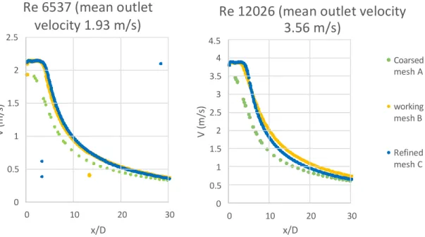
Mesh independence for model 1 was tested by comparing the centerline velocity profile at r/D=0 for Re 12026 and Re 6537. A minor difference between the chosen mesh and the refined mesh is seen as discussed in the previous paragraph and as shown by Figure 4 below.
2.5
Re 6537 (mean outlet
velocity 1.93 m/s)
Re 12026 (mean outlet velocity
3.56 m/s)
4.5 2 1.5 1 0.5 0 0 10 20 30 x/D 4 3.5 3 2.5 2 1.5 1 0.5 0 0 10 20 30 x/D Coarsed mesh A working mesh B Refined mesh C
Figure 4. Centerline velocity of Re 6537 (mean velocity 1.93 m/s) (left) and Re 12026 (mean V 3.56 m/s)
(right) at different meshes for model 1.
Noticeable change can be seen between the coarse and the working mesh particularly at the region x˂1. The variation deceases between the working and refined mesh.
3.1.2.2 Model 2
Mesh independence for model 2 was performed by comparing the centerline velocity profile for Re 2000 and Re 9233. A minor difference between the used mesh and the refined mesh is seen in figure 5.
V ( m /s ) V ( m /s )
1.6 1.4 1.2 1 0.8 0.6 0.4 0.2 0
Re 2000 (V▫ 1.39m/s)
0 10 20 30 x/DRe 9300( V▫ 6.43m/s)
7 6 5 4 Coarsed mesh D 3 Working mesh E 2 Refined mesh F 1 0 0 20 x/DFigure 5. The centerline streamwise velocity V 1.39 m/s -Re 2000 (left) and 6.43 m/s Re 9300 (right) at
different meshes for model 2.
3.1.2.3 Convergence and iterations
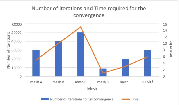
When refining the mesh, better results can be obtained. However, more iterations and more time will be required to obtain a complete convergence. The opposite is true. Hence, balancing the quality of the results, computation time and resources are crucial aspect to be considered when performing a CFD study. Figure 6 shows the number of iterations and the computational time required to obtain the convergence at each mesh.
Figure 6. Number of iterations and time at convergence for different meshes.
Mesh
Number of Iterations to full convergence Time
16 14 12 10 8 6 4 2 0 mesh F mesh E mesh D mesh C mesh B mesh A 60000 50000 40000 30000 20000 10000 0
Number of iterations and Time required for the
convergence
N um be r of ite rat io ns V ( m /s ) V ( m /s ) Ti m e in hr3.1.3 Inlet and boundary conditions
Inlet and boundary conditions for the two models were retrieved from two experimental studies that took place in the university of Gävle. The first study (Kabanshi and
Sandberg, 2019) experienced free round jet issuing from a smooth contraction nozzle with diameter 0.05m. Velocity was measured by a PIV system while the temperature was measured with T-type thermocouples. Likewise, the second study was carried out with a 0.025m nozzle diameter. Temperature was not measured for this study.
The measured velocity profiles at the nozzles exit are 2D top hat profiles and for this CFD study, they were transferred to a 3D cartesian velocity profile. The inlet velocities profiles were created in the field of 0≤θ≤90 with 5 degrees intervals. The generated velocities were U, V, and W. for this report the velocity at the horizontal axis X-direction is named U. The velocity at the Y-direction named W and the velocity at the vertical axis Z-direction is named Z. Equations 1,2, and 3 were used to calculate U, V, and W,
respectively.
U=u*cos (𝜃) ( 1)
V=v ( 2)
W=u*sin (𝜃) ( 3)
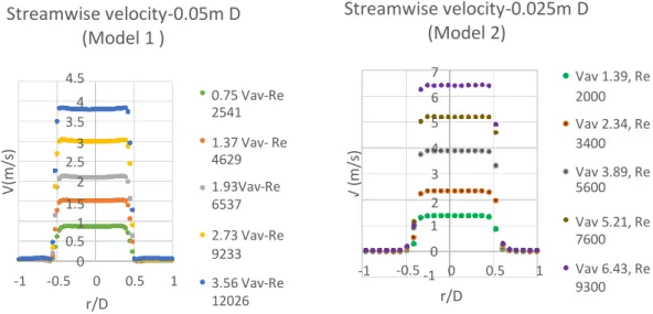
The streamwise and spanwise velocity profiles at the nozzle exit are shown by Figures 7 and 8 below. Streamwise velocity-0.05m D (Model 1 ) Streamwise velocity-0.025m D (Model 2) 4.5 7 Vav 1.39, Re 4 3.5 0.75 Vav-Re 2541 6 5 2000 Vav 2.34, Re V (m /s ) 3 2.5 2 1.37 Vav- Re 4629 1.93Vav-Re V (m /s ) 4 3 3400 Vav 3.89, Re 5600 1.5 6537 2 -1 1 0.5 0 -0.5 0 0.5 r/D 1 2.73 Vav-Re 9233 3.56 Vav-Re 12026 -1 1 0 -0.5 -1 0 r/D 0.5 1 Vav 5.21, Re 7600 Vav 6.43, Re 9300
Figure 7. The Streamwise velocity profile V in m/s at the nozzle exit for model 1 with 0.05m D (left) and
U
(m
/s
)
Figure 7 above shows the whole measured streamwise velocity at the nozzle exit. Whereas only half of the velocity profile at 0 ≤r≤ 0.5D has been used at the inlet face in this study.
Spanwise velocity-0.05m D
(Model 1)
Spanwise velocity-0.025m D
(Model B)
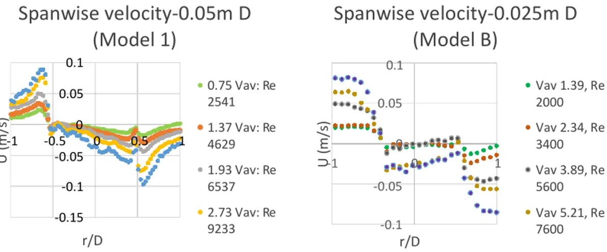
0.1 0.05 0 -1 -0.5 0 0.5 1 -0.05 -0.1 -0.15 r/D 0.75 Vav: Re 2541 1.37 Vav: Re 4629 1.93 Vav: Re 6537 2.73 Vav: Re 9233 r/D Vav 1.39, Re 2000 Vav 2.34, Re 3400 Vav 3.89, Re 5600 Vav 5.21, Re 7600Figure 8. The Spanwise velocity profile U in (m/s) used for models 1 (left) and 2(right).
Figure 8 shows the whole measured profile of the spanwise velocity at the nozzle exit. Similar to the streamwise velocity, the spanwise velocity profile in the region 0 ≤r/D≤0.5 has been used at the inlet face in this study.
Outlets were set as pressure outlets. The inner faces were set as symmetry. A steady-state and pressure-based solution were chosen for the simulations. The gravity and radiation influences were disabled for isothermal jets in case A (0.05m D) and case B (0.025mD). While gravity influence was considered in case C (non-isothermal flow at 0.05m D). Averaged discharged velocities, average turbulent intensities, and inlet and outlet temperatures are tabulated in table 3, 4, and 5. Reynolds numbers, Hydraulic diameters, and turbulent intensity were calculated by equations 4, 5, and 5.
Re=𝜌𝐷𝑉
𝜇
Where:
𝜌 : density of air D: nozzle diameter
V: mean velocity at the nozzle exit
𝜇 : kinematic viscosity of air
( 4) 0.1 0.05 0 -1 0 1 -0.05 -0.1 U (m /s )
Dh=4 𝑐𝑟𝑜𝑠𝑠−𝑠𝑒𝑐𝑡𝑖𝑜𝑛𝑎𝑙−𝑎𝑟𝑒𝑎 𝑜𝑓 𝑡ℎ𝑒 𝑛𝑜𝑧𝑧𝑙𝑒 =4 𝑤𝑒𝑡𝑡𝑒𝑑 𝑝𝑒𝑟𝑖𝑚𝑒𝑡𝑒𝑟 𝑜𝑓 𝑡ℎ𝑒 𝑛𝑜𝑧𝑧𝑙𝑒 𝜋𝐷2 4 = 𝐷 ( 5) 𝜋𝐷 Where: Dh=hydraulic diameter D=real diameter 𝑛 𝑖=1 Where: (𝑆𝑇𝐷)/𝑁 𝑉
TI= turbulence intensity
STD= standard deviation
V= velocity V
N=number of velocities
Table 3. Inlet boundary conditions for Case A-Model 1.
Average inlet velocity in m/s Reynolds number Initial turbulence intensity in % Temperature difference
between Inlet and outlet Hydraulic diameter in m 0.75 2541 6 0 0.05 1.37 4629 6 0 0.05 1.93 6537 7 0 0.05 2.73 9233 6 0 0.05 3.56 12026 5 0 0.05
Table 4. Inlet boundary conditions for case B- Model 2.
Average inlet velocity in m/s Reynolds number Initial turbulence intensity in % The temperature difference
between inlet and outlet Hydraulic diameter in m 1.39 2000 3.5 0 0.025 2.34 3400 2 0 0.025 3.89 5600 3 0 0.025 5.21 7600 2.6 0 0.025 6.43 9300 2.5 0 0.025 TI=∑ ( 6)
For case C, inlet temperature was set as 18.55±1 and outlet temperature was set as 22.25 ±1 .
Table 5. Inlet boundary conditions for 0.025m D (case B-Model 2): Velocity.
Average inlet velocity in m/s Reynolds number Initial turbulence intensity in % The temperature difference
between inlet and outlet Hydraulic diameter in m 0.75 2541 6 3.4 0.05 1.37 4629 6 4.1 0.05 1.93 6537 7 3.9 0.05 2.73 9233 6 3.4 0.05 3.56 12026 5 4 0.05
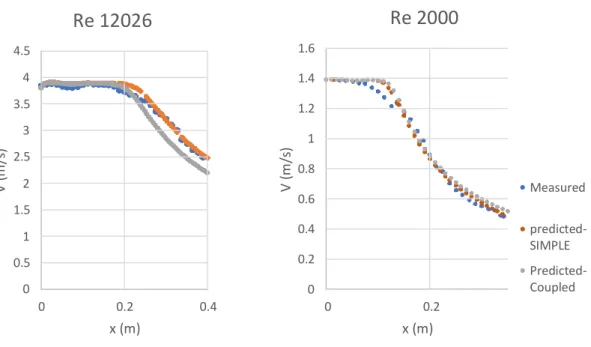
A finite volume solver was used for this study. Double precision, steady-state, and pressure-based solver was defined for the three studied cases. The air was modeled as an ideal gas and the second-order upwind scheme was used for the spatial discretization to obtain better accuracy. Under relaxation factor 0.3, 0.7, 0.8, and 0.8 were used for pressure, momentum, turbulent kinetic energy, and dissipation factor, respectively. A SIMPLE algorithm was chosen to solve the pressure velocity coupling for it is success in similar cases. Besides, the SIMPLE scheme was tested against a Couple scheme for the two models, and more accurate results when referring to the measured results were obtained by the former one compared to the latter one for the two models as shown in
Figure 9. Fluent ANSYS 2019 was used for the study. and all parameters were converged with residuals below e-6
4.5 4 3.5 3 2.5 2 1.5 1 0.5 0
Re 12026
0 0.2 0.4 x (m) 1.6 1.4 1.2 1 0.8 0.6 0.4 0.2 0Re 2000
0 0.2 x (m) Measured predicted- SIMPLE Predicted- CoupledFigure 9. the Streamwise velocity V 3.56m/s-Re 12026 in model 1 (left) and V 1.39-Re 2000 in model 2
(right) at different pressure velocity schemes.
3.2 Governing equation
The fluid motion is described by the conservation laws of mass, momentum, and energy in case of non-isothermal conditions. The energy equation is dropped when the flow is isothermal.
The mass conservation equation is called continuity while the momentum conservation law is an expression of Newton law and describes the equation of motion of the fluid. The energy conservation law is also an expression of the first principle of
thermodynamics. These equations when applied to viscous and perfect inviscid fluid are known as Navier-stokes equations and Euler equations respectively as shown in the publications of (Hirsch, 2007) and (Batchelor and Batchelor, 2000).
The most widely applied approximation of CFD is Reynolds Averaged Navier–Stokes equations whereby the turbulent equations are averaged out, in time, over the whole spectrum of turbulent fluctuations and Navier-stokes equations are solved in each control
V ( m /s ) V ( m /s )
volume. The incompressible Navier-Stokes equations in conservation form are given by the following equations retrieved from (Svensson, 2015)
𝜕𝑢𝑖 =0 ( 7) 𝜕𝑥𝑖 𝜕𝑢𝑖 +𝜕 (𝑢 𝑢 ) = − 1 𝜕𝑝 + 𝜈 𝜕 2𝑢 𝑖 − 𝜌𝔤∆𝑇 𝜕𝑡 𝜕𝑥𝑗 𝑖 𝑗 𝜌 𝜕𝑥𝑖 𝜕𝑥𝑖𝑥𝑗 ( 8)
The energy equation is given by
𝜌𝑐 𝜕𝑇 + 𝑐 𝑈 𝜕𝑇 𝜕2𝑇 𝜕 (−𝜌𝑐 𝑢 /𝑇/) +Q
𝑝 𝜕𝑡 𝑝 𝑗 𝜕𝑥𝑗
Where
= 𝜆 +
𝜕𝑥𝑖𝑥𝑗 𝜕𝑥𝑗 𝑝 𝑖 ( 9)
𝑐𝑝 is specific heat capacity at constant pressure. Q is heat source
T is temperature
For isothermal flow, the last right part of equation (8) is dropped and momentum is given by
𝜕𝑢𝑖 +𝜕 (𝑢 𝑢 ) = − 1 𝜕𝑝 + 𝜈 𝜕
2𝑢 𝑖
𝜕𝑡 𝜕𝑥𝑗 𝑖 𝑗 𝜌 𝜕𝑥𝑖 𝜕𝑥𝑖𝑥𝑗 ( 10)
𝑢𝑖 is velocity componenet in 𝑥𝑖 direction.
𝑝 is static pressure. 𝜈 is kinematic viscosity.
Equation 7 describes mass conservation in a fluid element and assume free divergence for incompressible fluids. While equation 10 describes momentum conservation. The
temporal change described by left hand side while change due to viscous forces and pressure is described by the right-hand side.
In turbulent flow, Reynolds decomposition is applied to flow and it is the consideration of instantaneous velocity 𝑢𝑖as a function of mean Ui and fluctuation component 𝑢𝑖/.
𝑖 𝑗
By putting equation 9 to Navier Stokes Equations (7) and (10) and using Reynolds averaging, Reynolds Average Navier Stokes equations RANS would yield as
𝜕𝑈𝑖 =0 ( 12) 𝜕𝑥𝑖 1 𝜕𝑝 𝜕 𝑈𝑖 𝜕𝑈𝑖 +𝜕 (𝑈 𝑈 ) = − + (𝜈 − ̅𝑢̅̅̅/𝑢̅ ̅̅̅/ ) 𝜕𝑡 𝜕𝑥𝑗 𝑖 𝑗 𝜌 𝜕𝑥𝑖 𝜕𝑥𝑗 𝜕𝑥𝑗 𝑖 𝑗 ( 13) 𝜅=1 ̅𝑢̅̅/̅ ̅𝑢̅̅̅/ ( 14) 2 𝑖 𝑗
Equation 13 used to calculate turbulent kinetic energy. And 𝑢̅ ̅̅/̅
̅𝑢 is Reynolds average
value.
Transportation equation for 𝜅 is given by
𝑖 𝑗
𝜕𝜅 + 𝜕𝜅𝑈𝑗
= −̅𝑢̅ ̅𝑢̅̅ 𝜕𝑈 𝜕 1 1 𝜕𝜅 ̅𝜕̅ ̅𝜕̅̅𝑢̅
𝑖 + (− 𝑢̅ 𝑢̅̅̅ 𝑢̅̅ − 𝑝 ̅̅ + 𝜈 ) + 𝜈 𝑖 𝑖
𝜕𝑡 𝜕𝑥𝑗 𝑖 𝑗 𝜕𝑥𝑗 𝜕𝑥𝑗 2 𝑖 𝑗 𝑖 𝜌 𝑗 𝜕𝑥𝑗 𝜕𝑥𝑗 𝜕𝑥𝑗 ( 15)
Left-hand side describes the temporal change.
̅𝑢̅ ̅𝑢̅̅ 𝜕𝑈𝑖 is the production term and describes conversion of the mean kinetic energy to
𝑖 𝑗 𝜕𝑥𝑗
turbulent kinetic energy (energy dedicated to large eddies).
1 ̅𝑢̅ ̅𝑢̅̅̅ 𝑢̅̅ is turbulent transport. 2 𝑖 𝑗 𝑖 1 ̅𝑝̅̅𝑢 ̅̅ is pressure diffusion. 𝜌 𝑗 𝜈 𝜕𝜅 𝜕𝑥𝑗 is molecular diffusion.
RANS equations simulate the flow by averaging its properties. And its unclosed equation because of 𝑅𝑒𝑦𝑛𝑜𝑙𝑑𝑠 𝑠𝑡𝑟𝑒𝑠𝑠 ̅𝑢̅ ̅𝑢̅̅ . The boussineq hypothesis is applied to relate the Reynolds stresses to the mean flow rate of strain and given by:
̅−̅̅𝑢̅̅𝑖/̅ ̅𝑢̅̅𝑗̅/= 2 𝜐𝑇 𝑆
𝑖 𝑗
− 2 𝑘𝛿𝑖𝑗 ( 16)
3
𝜐𝑇 is kinetic eddy viscosity. K is turbulent kinetic energy
𝛿𝑖𝑗 is rate of strain tensor and given by 𝛿𝑖𝑗 = 1/2(𝜕𝑈𝑖
+𝜕𝑈𝑗(
3.3 Turbulence model
Two equations models have been proven to reliably predict the flow in similar cases as shown by (Ghahremanian and Moshfegh, 2014). For this study, to define the optimum turbulence model, a sensitivity analysis with several turbulence models was performed and standard κ -ω was chosen for this CFD study.
In the 𝜅- 𝜔 model, the Kinematic eddy viscosity is given by 𝜐𝑇 = 𝑘
𝜔 ( 17)
Turbulence kinetic energy
𝜕𝑘 = 𝜏𝑖𝑗 𝜕𝑈𝑖 − 𝛽∗𝑘𝜔 + 𝜕 [(𝜐 + 𝜎∗𝜐
𝑇) 𝜕𝑘 ( 18)
𝜕𝑥𝑗 𝜕𝑥𝑗 𝜕𝑥𝑗 𝜕𝑥𝑗
Specific dissipation rate
𝑈𝑖 𝜕𝜔 = 𝛼 𝜔 𝜏𝑖𝑗 𝜕𝑈𝑖 − 𝛽𝜔2 + 𝜕 [(𝜐 + 𝜎𝜐
𝑇) 𝜕𝜔 ( 19)
𝜕𝑥𝑗 𝑘 𝜕𝑥𝑗 𝜕𝑥𝑗 𝜕𝑥𝑗
Coefficients values are shown by table 6 below.
Table 6. Coefficients of the turbulence model k-𝜔.
Constant Value
Alpha*_ inf 1
Alpha_ inf 0.52
Beta*_inf 0.09
Beta_i 0.072
TKE Prandtl number 2
SDR Prandtl number 2
Energy Prandtl number 0.85
Wall Prandtl number 0.85
Production limited clip factor 10 𝑈𝑖
3.3.1.1.1.1 Sensitivity analysis- turbulence model
Several turbulence models were tested: one equation, two equations κ-ε and κ -ω, and SST κ -ω SST, 3 Equations, and 4 equations. the two equations standard k-ω turbulence model predicted flow more reliably than other turbulence models particularly for model 1 (0.05m D). Where two equations models predicted flow with minor variation in model 2 (0.025m D). Therefore, the turbulence model and k-ω was chosen for the three cases A, B, and C because it gave the most reliable results when comparing to the measured results. Streamwise velocity decay at r/D=0 for velocities 3.56 m/s- Re 12026 (model A) and 1.39m/s -Re 2000 (model B) were tested at a variety of turbulence models and results were plotted against the measured data as shown by figure 10.
Re12026-V▫ 3.56 m/s (Model1)
4.5Re 2000-V▫ 1.39m/s
(Model 2)
4 3.5 3 2.5 2 1.5 1 0.5 0 0 0.1 0.2 0.3 x (m) Measured 1 equation spalart allmaras 2 equations k-Ꜫ 2 equations k-ω 2 equations SST k- ω 3 equations k-kl-ω 4 equations SST 1.6 1.4 1.2 1 0.8 0.6 0.4 0.2 0 0 0.1 0.2 0.3 x (m)Figure 10. the centerline (r/D=0) streamwise velocity V (m/s) for 3.56m/s Re 12026 (left) and Re 6537
(right) obtained by different turbulence models.
3.4 Validation of the CFD Models
The results predicted by the CFD models were validated against previously measured PIV data (Kabanshi and Sandberg, 2019) and a second unpublished study by the same author. The model was validated by comparing the axial and radial spanwise and streamwise velocities for case A (isothermal flow at 0.05m D) and case B (isothermal flow at 0.025m D). And the radial and axial temperature for case C (non-isothermal flow at 0.05m D). The percentage of the average error between the predicted and the measured data was calculated for the three cases in different axial distances in the region 0 up to 12D and at the axial centerline. The error was calculated by estimating the average variation at 10-15 points at each radial or axial line. The error percentage for streamwise
V ( m /s ) V ( m /s )
velocity V, spanwise velocity U, and temperature was calculated according to equations 20, 21, and 22, respectively. 𝑉𝑒𝑟𝑟𝑜𝑟 𝑈 𝑛 𝑖=1 = ∑𝑛 𝑉𝑝𝑟𝑒𝑑𝑖𝑐𝑡𝑒𝑑−𝑉𝑚𝑒𝑎𝑠𝑢𝑒𝑑 % ( 20) 𝑉 𝑎𝑏𝑠𝑜𝑙𝑢𝑡𝑒 𝑉𝑝𝑟𝑒𝑑𝑖𝑐𝑡𝑒𝑑−𝑉𝑚𝑒𝑎𝑠𝑢𝑒𝑑 % ( 21) 𝑒𝑟𝑟𝑜𝑟 𝑖=1 U 𝑎𝑏𝑠𝑜𝑙𝑢𝑡𝑒 𝑇 = ∑𝑛 𝑉𝑝𝑟𝑒𝑑𝑖𝑐𝑡𝑒𝑑−𝑉𝑚𝑒𝑎𝑠𝑢𝑒𝑑 % ( 22) 𝑒𝑟𝑟𝑜𝑟 𝑖=1 T 𝑎𝑏𝑠𝑜𝑙𝑢𝑡𝑒
The measured and the predicted quantities were plotted for the three cases A, B, and C. and calculated variation was tabulated. In this section, results for validation at the inlet (nozzle exit) and at the centerline (r/D=0) will be shown. The full validation profile with charts and a more detailed table can be found in Appendix A.
Table 7. Validation results of model 1(0.05m D)-isothermal flow.
Average velocity in m/s Reynolds number Radial streamwise average error % Axial streamwise average error (r/D=0) % Radial spanwise average error % Axial spanwise average error % (r/D=0) 0.75 2541 6.6 2.6 0.7 0.8 1.37 4629 5.8 3.7 0.7 0.4 1.93 6537 5.1 5.4 0.6 0.9 2.73 9233 5 4.6 0.4 0.8 3.56 12026 2.9 1.2 0.6 0.6
Table 8. Validation results of Model 1(0.05m D) by scaling Temperature (case C).
Average velocity in m/s Reynolds number Radial temperature average error % Axial temperature average error (r/D=0) % 0.75 2541 1 1 1.37 4629 1 1 1.93 6537 1 1 2.73 9233 1 1 3.56 12026 1 1 =∑
Table 9. Validation results of model 2 (0.025m D)-scaling velocity (case B). Average velocity in m/s Reynolds number Radial streamwise average error % Axial streamwise average error (r/D=0) % Radial spanwise average error % Axial spanwise average error (r/D=0) % 1.39 2000 2.4 2 0.6 0.9 2.34 3400 5 6 0.6 0.8 3.89 5600 3.3 6 0.4 0.4 5.21 7600 3 8 0.5 0.3 6.43 9300 3 9 0.5 0.3
Plots of measured against predicted (CFD) velocities and temperature profiles are shown by figures below. Complete profile of validation plots is available in appendix A.
3.4.1 Model 1-case A (isothermal flow at 0.05m D)
Measured and predicted velocities for (case A) isothermal flow at 0.05m D were obtained and can be seen in this section.
Measured and predicted mean streamwise velocity at the nozzle exit
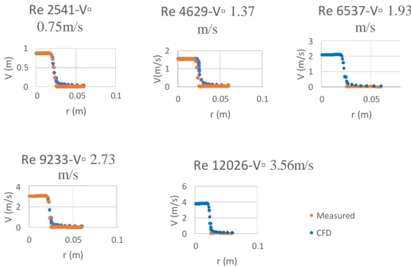
The predicted and measured streamwise velocities at the nozzle exit (x/D=0) for the different Re flows in 0.05m D (case A) are shown by figure 11.
1 0.5 0
Re 2541-V▫
0.75m/s
0 0.05 0.1 r (m)Re 4629-V▫ 1.37
m/s
2 1 0 0 0.05 0.1 r (m)Re 6537-V▫ 1.93
m/s
3 2 1 0 0 0.05 r (m)Re 9233-V▫ 2.73
m/s
4 2 0 0 0.05 0.1 r (m)Re 12026-V▫ 3.56m/s
6 4 2 0 0 0.1 r (m) Measured CFDFigure 11. The Measured and predicted streamwise velocity profile at the nozzle exit for different Re flows
within 0.05 m D (case A)
Figure 11 shows a strong correlation between the measured and the predicted velocities at the inlet (nozzle exit).
V ( m /s ) V ( m ) V (m /s ) V ( m /s ) V ( m /s )
Measured and predicted mean spanwise velocity at the nozzle exit 0.1 0 -0.1
Re 2541
r (m)Re 9233
0.05 0 -0.05 -0.1Re 4629
0 0.1 r (m)Re 12026
0.05 0 -0.05 -0.1Re 6537
0 0.05 0.1 r (m) 0.05 -0.05 -0.15 0 0.05 0.1 r (m) 0.05 0 -0.05 -0.1 0 0.1 r (m) Measured PredictedFigure 12. The Measured and predicted spanwise velocities at the nozzle exit (x/D=0) for different Re
flows within 0.05m D (case A).
Although the small values of U velocities, CFD showed a good prediction at the model inlet (nozzle exit) except for Re 4629 as can be seen in figure 12.
Measured and predicted mean streamwise velocity at the axial centerline (r/D=0)
Streamwise and spanwise velocity at the axial centerline (r/D=0) for different Re flows were explored and the obtained profiles were plotted as shown by figure 13.
0 0.1 U (m /s ) U (m /s ) U (m /s ) U (m /s ) U (m /s )
1 0.5 0
Re 2514
0 0.5 x (m) 2 1.5 1 0.5 0Re 4629
0 0.5 x (m)Re 6537
3 2 1 0 0 0.5 x (m)Re 9233
4 2 0 0 0.5 x (m)Re 12026
6 4 2 0 0 0.5 x (m) measured CFDFigure 13. The Measured and predicted streamwise velocities for different Re flows at the axial centerline
(r/D=0) within 0.05m D (case A).
Figure 13 illustrate a good agreement between the mean centerline measured and predicted streamwise velocities.
Measured and predicted mean spanwise velocity at the axial centerline (r/D=0)
0.05 0
Re 2541
Re 4629
0.05 0Re 6537
0.05 0 -0.05 0 0.2 0.4 0.6 x (m) -0.05 0 0.5 x (m) -0.05 0 0.5 x (m) 0.05 0 -0.05Re 9233
x (m) 0.05 0 -0.05Re 12026
x (m) Measured Predicted-CFDFigure 14. The Measured and predicted mean spanwise velocities at axial centerline (r/D=0) for different
Re flows at 0.05m D (case A).
0 0.2 0.4 0.6 0 0.5 V ( m /s ) V ( m /s ) U (m /s ) U( m /s ) U (m /s ) V ( m /s ) U( m /s ) V (m /s ) U( m /s ) V (m /s )
The Figures 11, 12, 13 above show a good agreement between the predicted and the measured velocities at the nozzle exit and at the axial centerline (r/D=0) for the
streamwise V velocities. However, variation can be spotted between the predicted and the measured spanwise U velocities (see figure 14). On one hand, when looking at the
scattered distribution of the measured velocities the axial centerline and knowing that U velocities were measured with a PIV system with around 2% uncertainty (Kabanshi and Sandberg, 2009) arise a possibility of uncertainty due to instability conditions associated with measurements. The predicted U velocities are still within the range of the measured velocities +/- 2%. On the other hand, RANS models may be unable to capture and predict accurately the very low spanwise velocities while developing at the centerline.
3.4.2 Model 1-Case B (non-isothermal flow-0.05m D)
In case B, non-isothermal flow issuing from a 0.05m nozzle diameter (model1) was studied. The measured and predicted temperatures were compared and plotted as shown in this section.
Measured and predicted temperature at the nozzle exit
The predicted and measured temperatures were obtained at the nozzle exit (inlet face) and at the axial centerline as shown by the figures 15 and 16 below.
Re 2541
23 21 19 17Re 4529
23 21 19 17Re 6537
23 21 19 17 0 0.5 0 r (m) r (m) 0.5 0 r (m) 0.5Re 9233
23 21 19 17 0 0.5 r(m)Re 12026
23 21 19 17 0 0.5 r (m) Measured Predicted-CFDFigure 15. The Measured and predicted temperature at the nozzle exit for different Re flows within 0.05m
D (case C). T ( ̊ C) T ( ̊ C) T ( ̊ C) T ( ̊ C) T ( ̊ C)
Measured and predicted temperature at the axial centerline (r/D=0)
Re 2541
22 20 18 0 0.5 x (m)Re 4629
22 21 20 19 18 0 0.2 0.4 x (m)Re 6537
22 21 20 19 18 0 0.2 0.4 x (m)Re 9233
21 20 19 18 0 0.5 x (m)Re 12026
21 20 19 18 17 0 0.5 x (m) Measured CFDFigure 16. The Measured and predicted temperature at the axial centerline (r/D=0) for different Re flows
within 0.05m D (case C).
The figures above show a good agreement between the measured and predicted
temperatures at the nozzle exit and at the axial centerline (r/D=0). The complete profile of temperature at the other distances is available in appendix A.
3.4.3 Model 2 - Case B (isothermal flow-0.025m D)
The measured and predicted streamwise and spanwise velocities were obtained for model 2 where air is issuing from 0.025 m diameter and plotted in figure 17 and 18.
T ( ̊ C) T ( ̊ C) T ( ̊ C) T ( ̊ C) T ( ̊ C)
0 0.05 0.1
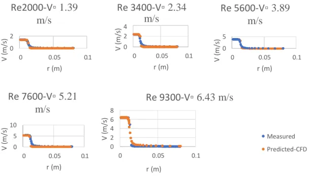
Measured and predicted mean streamwise velocity at the nozzle exit (x/D=0)
Re2000-V▫ 1.39
m/s
2 0 0 0.05 0.1 r (m)Re 3400-V▫ 2.34
m/s
4 2 0 0 0.05 0.1 r (m)Re 5600-V▫ 3.89
m/s
5 0 0 0.05 0.1 r (m)Re 7600-V▫ 5.21
m/s
10 5 0 0 0.05 0.1 r (m)Re 9300-V▫ 6.43 m/s
8 6 4 2 0 0 0.05 0.1 r (m) Measured Predicted-CFDFigure 17. The Measured and predicted mean streamwise velocity at the nozzle exit (x/D=0) for the
different Re flows within 0.025m D (case B).
Measured and predicted mean spanwise velocity at the nozzle exit (x/D=0)
0.02 0 -0.02
Re 2000
r (m) 0.04 0.02 0 -0.02 -0.04Re 3400
0 0.05 0.1 r (m) 0.05 0 -0.05 -0.1Re 5600
r (m) 0.2 0 -0.2Re 7600
0 0.05 0.1 r (m) 0.2 0 -0.2Re 9300
r (m) Measured Predicted-CFDFigure 18. The Measured and predicted mean spanwise velocity at nozzle exit for different Re at 0.025m D
(case B). 0 0.05 0.1 0 0.05 0.1 U (m /s ) U( m /s ) V ( m /s ) V ( m /s ) V ( m /s ) U (m /s ) U (m /s ) V ( m /s ) U (m /s ) V ( m /s )
Good agreement between the measured and the predicted mean velocities at the nozzle exit can be seen from figures 17 and 18. Some variation for Re 2000 at the nozzle exit can be spotted.
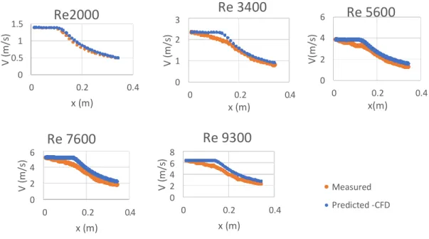
Measured and predicted mean streamwise velocity at the axial centerline (r/D=0)
1.5 1 0.5 0
Re2000
0 0.2 0.4 x (m)Re 3400
3 2 1 0 0 0.2 0.4 x (m) 6Re 5600
4 2 0 0 0.2 0.4 x(m)Re 7600
6 4 2 0 0 0.2 0.4 x (m)Re 9300
8 6 4 2 0 0 0.2 0.4 x (m) Measured Predicted -CFDFigure 19. The Measured and predicted streamwise velocity at the axial centerline r/D=0 for the different
Re flows within 0.025m D (case B).
V ( m /s ) V ( m /s ) V ( m /s ) V ( m /s ) V (m /s )
Measured and predicted spanwise velocity at the nozzle exit (x/D=0) 0.02 0 -0.02 -0.04 -0.06
Re 2000
0 0.2 0.4 x (m)Re 3400
0.1 0.05 0 -0.05 x (m) 0.1 0.05 0 -0.05Re 5600
x (m) 0.1Re 7600
0.1Re 9300
0 -0.1 x (m) 0 -0.1 x (m) Measured Predicted CFDFigure 20. The Measured and predicted mean spanwise velocity at the axial centerline r/D=0 for the
different Re flows within 0.025m D (case B).
Like case A, the above figures show a good agreement between the predicted and the measured velocities at the axial centerline (r/D=0) for the mean streamwise V velocities and variation with mean spanwise velocity U can be seen. This was discussed previously (see spanwise velocity for case A).
0 0.2 0.4 0 0.2 0.4 0 0.2 0.4 0 0.2 0.4 U (m /s ) U (m /s ) U (m /s ) U (m /s ) U (m /s )
4 Results and discussion
4.1 Vector field
4.1.1 The velocity contours
The streamwise velocity V was normalized with the maximum velocity for different Re jets within 0.05m D (case A) and 0.025 m D (case B) and the contour of the normalized velocities obtained. For better pictures that clearly catches the jet distribution, contour length is limited to 15 D downstream where the major development of the jet occurs. Figure 21 and 22 show velocity contours for 0.05m D (case A) and 0.025m D (case B) respectively.
Re 2541 Re 4629 Re 6537 Re 9233 Re 12026
Figure 21. The contour of the normalized velocity (V/Vm) for different Re jets flows at 0.05m D (case A).
In figure 21, nearly similar potential length can be seen for Re 4629, 9233, and 12026. For these jets, the maximum potential length is clearly seen. which suggest an extension of the exit conditions and presumably higher penetration distance for the three jets. Re 2541 has the shorter potential length but noticeably higher spread.
Re 2000 Re 3400 Re 5600 Re 7600 Re 9300
V
/V
m
For 0.025m D (case B), Figure 22 shows a minor small variation in the potential length and spread. a gradual increase in potential length with Re increase can be seen. Further discussion of velocity distribution in the next sections.
4.1.2 Radial distribution of the mean streamwise velocity
To understand jet behavior outward, the radial distribution of the stream velocity V was studied by exploring the radial streamwise (V) and spanwise (U) velocities with 0.05m D (case A) and 0.025m D (case B) at different axial distances in the region 0≤x/D≤30. Velocity spread outward is shown by figures 23 and 24 below.
1 0.5 0
x/D=0
0 2 4 r/D 1 0.5 0x/D=4
0 2 4 r/D 1 0.5 0x/D=14
0 2 4 r/D 1 0.5 0x/D=20
0 2 4 r/D 1 0.5 0x/D=30
0 2 4 r/D 2514 4629 6537 9233 12026Figure 23. The radial streamwise velocity V normalized with maximum velocity Vm at different axial
locations for the different Re flows within 0.05m D (case A).
V /V m V /V m V /V m V /V m
1 0.8 0.6 0.4 0.2 0 1 0.8 0.6 0.4 0.2 0
x/D=0
0 1 2 r/Dx/D=20
0 2 4 r/D 1 0.8 0.6 0.4 0.2 0 1 0.8 0.6 0.4 0.2 0x/D=4
0 1 2 r/Dx/D=30
0 2 4 r/D 1 0.8 0.6 0.4 0.2 0 x/D=14 0 2 4 r/D Re 2000 Re 3400 Re 5600 Re 7600 Re 9300Figure 24. The radial distribution of mean streamwise velocity V normalized with maximum velocity Vm at
different axial locations for the different Re flows within 0.025m D (case B).
By studying figures 23 and 24, several points can be reported. A top hat velocity profile can be seen at the nozzle exit (x/D=0) for all jets and gradually diffuses out to a Gaussian profile at x/D=4. As moving downstream, velocity spread outward but with a decreasing value due to jet flow mixing with surrounding stagnant fluid. Eventually, and as the jet is mixed with the surrounding the curve tends to flatten at x/D=30.
Re spread dependency can be seen although the small variation among the velocity magnitude. Literature suggests that high Re jets have higher velocity in the outer region (Milanovic and Hammad, 2010). This can clearly be seen at the centerline and up to 0.7D outward while it is not obvious in the outer region where Re jets superimposed over others.
4.1.3 Axial centerline mean velocity
Development of streamwise velocity in the axial centerline (r/D=0) was studied and the streamwise velocity V was normalized with the maximum velocity Vm and plotted versus axial distance x as shown by figures 25 and 26.
V /V m V /V m V /V m V /V m V /V m
centerline streamwise velocity for 0.05m
D (case A)
1.2 1 0.8 Re 2541 0.6 Re 4629 0.4 Re 6537 Re 9233 0.2 Re 12026 0 0 5 10 15 x/D 20 25 30Centerline streamwise velocity for
0.025m D (case B)
1.2 1 0.8 0.6 0.4 0.2 Re 2000 Re 3400 Re 5600 Re 7600 Re 9300 0 0 5 10 15 x/D 20 25 30Figure 25. The mean centerline streamwise velocity V normalized with the maximum mean velocity Vm for
different Re flows within 0.05m D (case A) at r/D=0.
Figure 26. The mean streamwise velocity V normalized with the maximum mean velocity Vm for different
Re flows within 0.025m D (case B)
V /V m V /V m
In the initial region of the centerline layer, velocity V is not decaying presumably due to no mixing occurs there because of the low turbulence structure in this region as a result of low turbulent kinetic energy (see Figures 33 and 34) in TKE section. A potential core region where velocity is nearly constant is a typical feature of contraction nozzles. In this region, jet features meet those of the surrounding mixing zone (Batchelor and Batchelor, 2000). The potential core region found at 0˂x/D ≤3.5 to 4.5 for case A and at 0≤x/D≤5 to 6 for 0.05 m D for case B. The potential length is nearly the same for the studied jets except for Re 9233 and 12026 in case A and 7600 and 9300 in case B. High Re jets have lengthier potential region. This can be linked to the low initial turbulence intensity associated with high Re jets or higher velocities. And it suggests that the exit conditions at these relatively high Re jets are extended further downstream and consequently have a higher penetration distance. Relatively short potential length can be seen in Re 6537 compared to potential length at Re 4629. This could be due to the relatively high initial turbulence intensity TI (at the nozzle exit) which estimated from the measured data (see Table 3).
As moving downstream, the turbulent structures generated in the shear layer reach the jet centerline at the tip of the potential core. As a result, the velocity starts to decay. The inverse normalized velocity (Vm/V) was plotted and the slope was estimated and listed in table 10 below. (The inverse velocity decay available in Appendix B).
Table 10. slope of inverse velocity decay at the axial centerline (r/D=0) for different Re flows.
Re- 0.05m D (Case A)
Linear slope Re- 0.025m D (case B) Linear slope 2541 0.1875 2000 0.1562 4629 0.1552 3400 0.1576 6537 0.2026 5600 0.147 9233 0.1515 7600 0.1433 12026 0.1453 9300 0.1416
The major decay by 12% occurs at the tip of the potential core up to 10D downstream. This may be used as an indication of the transitional region where flow transit from laminar to turbulent. At x/D>10, jets decay with a decreasing rate. Re-velocity decay dependency can be seen in the region up to 25 D downstream and similarity is obtained beyond this distance. In general, as Re increases, the velocity decay decreases (see table 10). A similar finding was reported by many studies (Oosthuizen, 1984) and (Abdel- Rahman, Al-Fahed and Chakroun, 1996). Less jet decaying among high Re flows occurs because of the small eddies which are dominating high Re flows and which have less pronounced mixing and consequently less velocity decay (Kabanshi and Sandberg, 2019).
Re 6537 showed unexpected relatively high decay which reflecting a high jet mixing. This can be due to the highest initial turbulence intensity measured at Re 6537 (see table 3). The initial turbulence approved to influence velocity decay (Lemieux and Oosthuizen, 1985).
Figure 27.centerline mean streamwise velocity for nearly similar Re jets with different discharge velocities.
When looking at nearly equal Reynolds jets Re 2000 (mean velocity 1.39 m/s) and Re 2541 (mean velocity 0.75 m/s), and Re 9233 (mean velocity 2.73 m/s) and Re 9300 (mean velocity 6.43 m/s), less decay can be seen at Re jets with higher velocity.
Suggesting a less turbulence intensity for higher velocity jet. This can be due to the low turbulence associated with high velocities and demonstrated by the initial low turbulence at nozzle exit. It suggests that initial conditions have an extended influence on jet
development (see tables 3 and 5). This complies with was reported by ((Malmstrom, Kirkpatrick, Christensen and Knappmiller, 1997) who stated that velocity decay is a function of the outlet velocity rather than the Re number.
U/
V
m
4.1.4 Radial distribution of the spanwise velocity
0.03 0.01 -0.01 -0.03
x/D=0
0 5 10 r/D 0.03 0.01 -0.01 -0.03x/D=2
0 5 10 r/D 0.03 0.01 -0.01 -0.03x/D=10
0 5 10 r/D 0.03 0.01 -0.01 -0.03x/D=20
0 5 10 r/D 0.03 0.01x/D=30
2541 4629 6537 9233 -0.01 -0.03 0 5 10 r/D 12026Figure 28. The spanwise velocity normalized with the maximum streamwise velocity at different distances
for Re flows at 0.025m D (case B).
U/ V m U/ V m U/ V m U/ V m