Experimental Studies of Thermal Diffusivities concerning some Industrially Important Systems

Experimental Studies of the

Thermal Diffusivities concerning

some Industrially Important Systems

Riad Abdul Abas

Doctoral Thesis in

Metallurgical Process Science

Stockholm, Sweden 2006

ISRN KTH/MSE--05/96—SE+ THMETU/AVH

ISBN 91-7178-251-6

RIAD ABDUL ABAS Experimental Studies of the Thermal Diffusivities concerning some Industrially Important Systems. KTH 2006

Experimental Studies of the Thermal Diffusivities concerning

Some Industrially Important Systems

Riad Abdul Abas

Doctoral Dissertation

School of Industrial Engineering and Management Department of Material Science and Engineering

Royal Institute of Technology SE-100 44 Stockholm Sweden

________________________________________________________________ Akademisk avdelning som med tillstånd av Kungliga Tekniska Högskolan i Stockholm, framlägges för offentlig granskning för avläggande av Teknologie

doktorsexamen, torsdag den 16 mars 2006, kl.10:00 i F3 , Lindstedsvägen 26, Kungliga Tekniska Högskolan, Stockholm

________________________________________________________________________

ISRN KTH/MSE--05/96--SE+THMETU/AVH ISBN 91-7178-251-6

Riad Abdul Abas. Experimental Studies of the Thermal Diffusivities concerning Some Industrially Important Systems

School of Industrial Engineering and Management Department of Material Science and Engineering Royal Institute of Technology

SE-100 44 Stockholm Sweden

ISRN KTH/MSE--05/96--SE+THMETU/AVH ISBN 91-7178-251-6

ABSTRACT

The main objective of this industrially important work was to gain an increasing understanding of the properties of some industrially important materials such as CMSX-4 nickel base super alloy, 90Ti.6Al.4V alloy, 25Cr:6Ni stainless steel, 0.7% carbon steel, AISI 304 stainless steel-alumina composites, mould powder used in continuous casting of steel as well as coke used in blast furnace with special reference to the thermal diffusivities. The measurements were carried out in a wide temperature range covering solid, liquid, glassy and crystalline states.

For CMSX-4 alloy, the thermal conductivities were calculated from the experimental thermal diffusivities. Both the diffusivities and conductivities were found to increase with increasing temperature. Microscopic analysis showed the presence of intermetallic phases γ´ such as Ni3Al below 1253 K. In this region, the

mean free path of the electrons and phonons is likely to be limited by scattering against lattice defects. Between 1253 K and solidus temperature, these phases dissolved in the alloy adding to the impurities in the matrix, which, in turn, caused a decrease in the thermal diffusivity. This effect was confirmed by annealing the samples at 1573 K. The thermal diffusivities of the annealed samples measured at 1277, 1403 and 1531 K were found to be lower than the thermal diffusivities of non-annealed samples and the values did not show any noticeable change with time. It could be related to the attainment of equilibrium with the completion of the dissolution of γ´ phase during the annealing process. Liquid CMSX-4 does not show any change of thermal diffusivity with temperature. It may be attributed to the decrease of the mean free path being shorter than characteristic distance between two neighbouring atoms.

Same tendency could be observed in the case of 90Ti.6Al.4V alloy. Since the thermal diffusivity increases with increasing temperature below 1225 K and shows slight decrease or constancy at higher temperature. For 25Cr:6Ni stainless steel, the thermal diffusivity is nearly constant up to about 700 K. Beyond that, there is an increase with temperature both during heating as well as cooling cycle. On the other hand, the slope of the curve increases above 950 K, which can be due to the increase of bcc phase in the structure. 0.7% carbon steel shows a decrease in the thermal diffusivity at temperature below Curie point, where the structure contains bcc+ fcc phases. Above this point the thermal diffusivity increases, where the structure contains only fcc phase. The experimental thermal conductivity values of these alloys show good agreement with the calculated values using Mills model.

Thermal diffusivity measurements as a function of temperature of sintered AISI 304 stainless steel-alumina composites having various composition, viz, 0.001, 0.01, 0.1, 1, 2, 3, 5, 7, 8 and 10 wt% Al2O3 were carried

out in the present work. The thermal diffusivity as well as the thermal conductivity were found to increase with temperature for all composite specimens. The thermal diffusivity/conductivity decreases with increasing weight fraction of alumina in the composites. The experimental results are in good agreement with simple rule of mixture, Eucken equation and developed Ohm´s law model at weight fraction of alumina below 5 wt%. Beyond this, the thermal diffusivity/ conductivity exhibits a high discrepancy probably due to the agglomeration of alumina particles during cold pressing and sintering.

On the other hand, thermal diffusivities of industrial mould flux having glassy and crystalline states decrease with increasing temperature at lower temperature and are constant at higher temperature except for one glassy sample. The thermal diffusivity is increased with increasing crystallisation degree of mould flux, which is expected from theoretical considerations.

Analogously, the thermal diffusivity measurements of mould flux do not show any significant change with temperature in liquid state. It is likely to be due to the silicate network being largely broken down.

In the case of coke, the sample taken from deeper level of the pilot blast furnace is found to have larger thermal diffusivity. This can be correlated to the average crystallite size along the structural c-axis, Lc,

which is indicative of the higher degree of graphitisation. This was also confirmed by XRD measurements of the different coke samples. The degree of graphitisation was found to increase with increasing temperature. Further, XRD and heat capacity measurements of coke samples taken from different levels in the shaft of the pilot blast furnace show that the graphitisation of coke was instantaneous between 973 and 1473 K.

Keywords: laser flash, thermal diffusivity, heat conduction, phonon, electron contribution, crystallisation degree, graphitisation.

ACKNOWLEDGMENT

First I would like to thank my advisor Prof. Seshadri Seetharaman for his excellence as scientist and scientific adviser. I will never forget how you adopt me as your son, when I was with out any support of anybody. During the difficult time of me, my family and my country, your words were the suitable balm of my suffering.

Special thanks to Professor Mamoun Muhammed for encouragement and the valuable support throughout the work.

I am also grateful to Prof. Miyuki Hayashi for fruitful discussions and inspiring ideas. Thanks are also due to, Dr. Ragnhild Aune, Dr. Robert Eriksson, Dr. Abdulsalam Uheida and Dr. Anders Jakobsson for their valuable help.

My sons Wasim and Mohammed and my daughter Rokeia. Thank you for all your smiles, which give me a greatest happiness in life.

I would like to thank my family and my friends in Iraq and Sweden for their prayers and encouragement.

I thank all my colleagues working with material science in the department.

Riad Harwill Abdul Abas Stockholm, February 2006

Supplements

The present thesis is based on the following papers:

Suppliment 1: Thermal Diffusivity measurement of CMSX-4 alloy by Laser flash method

R. Abdul Abas, M. Hayashi and S. Seetharaman

Submitted to International Journal of Thermophysics, USA, 2005

Suppliment 2: Thermal Diffusivity Measurements of some Industrially Important Alloys by a Laser Flash Method

R. Abdul Abas, M. Hayashi and S. Seetharaman Submitted to Zeitschrift fur Metallkunde, Germany, 2005

Suppliment 3: Thermal Diffusivity of Sintered Stainless steel-Alumina Composite. R. Abdul Abas and S. Seetharaman

Accepted for publication in Journal of Metallurgical and Materials Transactions, USA, January 2006

Supplement 4: Effect of Crystallinity on the Thermal Diffusivity of Mould Fluxes for the Continuous Casting of Steels.

M. Hayashi, R. Abdul Abas and S. Seetharaman

ISIJ International, Vol. 44 (2004), No. 4 (April), pp. 691-697.

Supplement 5:

Studies on Graphitisation of Blast Furnace Coke by X-ray Diffraction Analysis and Thermal Diffusivity Measurements

R. Abdul Abas, A. Jakobsson, M. Hayashi and S. Seetharaman Submitted to Steel Research, Germany, 2005.

The author’s contribution to the papers of the thesis:

І. Literature survey, experimentation and major part of the writing.

ІІ. Literature survey, theoretical analyses, experimentation and major part of the writing.

ІІІ. Literature survey, experimentation and major part of the writing.

IV. Experimentation, result evaluation, participates in the theoretical analysis.

V. Experimental work, analysis and evaluation of the experiment results and the major part of the writing.

TABLE OF CONTENTS

1. INRODUCTION………1 1.1 Industrial importance ……….…3 2. EXPERIMENTAL ……….………5 2.1 Experimental techniques..………..……….………5

2.1.1. Laser flash method ……….…….……5

2.1.2 X-ray diffraction techniques. ………..…….8

2.1.3. Calorimetric technique………..……….……..9

2.2 Material and samples preparation………..…….……….….…………..10

2.2.1. Alloys………10

2.2.2. Composites ……….………10

2.2.3. Mould powder ……….…...…11

2.2.4. Coke ……… ………12

3. RESULTS AND DISCUSSION…….…………..………....……..15

3.1 Thermal diffusivity of alloys ………..………….…15

3.1.1. CMSX-4 alloy……….……..15

3.1.2. 90Ti.6Al.4V alloy………22

3.1.3. 25Cr:6Ni stainless steel ………...….25

3.1.4. 0.7% carbon steel ………. 28

3.1.5. Electron contribution of thermal conduction of alloys...31

3.2 Composites ………..………..….32

3.3 Mould powder………..……..…….40

3.3.1 XRD measurements………..…....….….40

3.3.2 Thermal diffusivity measurements……….……..……..41

3.4 Coke……….…..…....…….45

3.4.1 XRD measurements……….……..…….……45

3.4.2 Heat capacity measurements……….……….……….48

3.4.3 Thermal diffusivity measurements………...…………...………49

3.5. General discussion……….…..…………..………52

4. CONCOLUSION………..………….……55

5. FUTURE WORK……….………..57 REFERENCES

1. INTRODUCTION

Thermophysical properties such as thermal diffusivity, viscosity and heat capacity are very important from both fundamental as well as practical view points. There are many engineering situations in which the ability of a structural component to either dissipate a large quantity of locally generated heat or conduct heat to/from a material such as ferrous and non-ferrous alloys, metallic matrix composites, mould flux used in continuous casting of steel and blast furnace coke or is of fundamental importance. It is therefore, necessary to determine the thermal transport properties of such materials. If, however improvements in engineering efficiency are to be achieved by improving the heat transfer characteristics, it becomes necessary to understand how, for the material under investigation, heat transport is affected by changes in structure or in the relative proportion of phase’s present [1].

In recent years, mathematical modeling of the heat transfer mechanism occurring in high temperature processes has resulted in improvements in process control such as steelmaking and production of heat resistance materials such as Ni-base super alloy and Ti-base alloys. However, reliable values for the thermophysical properties of materials involved are required for the successful operation of these models [2].

The problem of determining the effective thermal conductivity of randomly packed granular materials is one which frequently occurs in engineering practice. A detailed solution of the conduction problem would require knowledge of the shape, size, location and conductivity of each particle in the system together with the interaction between particles. From simplifying hypotheses regarding the dispersion of the discontinuous phase, an overall value of the thermal conductivity can be obtained for a unit cube of the mixture [3].

In the continuous casting of steels, one of the factors affecting the surface quality of the product is the heat transfer process occurring in the mould. It is dominantly influenced by the characteristics of the mould powder infiltrated into the mould/strand gap. The mould powder forms a slag film between mould and solidified steel shell, which frequently consists of glassy, crystalline and liquid layers. Because of the importance of the thermal diffusivity values of slags in heat transfer modeling, they have been measured by different researchers. With respect to the thermal conductivities/ diffusivities of mould flux powder in the glassy and crystalline state, there are very few previous reports available. Shibata et al [4] and Taylor and Mills [5] have reported that the thermal diffusivities of the crystalline samples are higher than those of the glassy samples. However, since the thermal conductivities/ diffusivities of solid slag are considered to be dependent on crystallinity of the samples. Thus, the property should be measured as a function of the degree of crystallisation as well as temperature. Because of the experimental difficulties at high temperature, there are very few accurate data of such properties.

To optimize the blast furnace process, the coke quality and coke consumption rate must be improved. One major factor affecting the coke quality is the degree of graphitisation. It was reported that the higher degree of graphitisation leads to lower reactivities [6, 7]. Earlier studies of the thermal diffusivities of coke samples indicate that, the thermal diffusivity of the coke increases with increase the graphitisation degree of the coke [8, 9]. It is critical to the optimum performance of the furnace to focus on the factors, which could affect the degree of graphitisation. These factors can be temperature, chemical composition and thermal history of the coke.

The methods for measuring the thermal diffusivity can be classified into two main groups: viz. periodic and nonperiodic heat flow methods.The periodic method includes Ångström, thermoelectric and radial wave methods, while the nonperiodic method includes bar, small area, semi-infinite plate, radial heat flow high-intensity arc, electrically-heated rod and flash method [10]. Most of these methods have inherent limitations primarily due to heat transport via convection as well as heat loses by radiation at elevated temperatures. The impact of these factors is minimized by laser flash technique, which is one of the transient methods,due to the small thickness of the sample and the high-speed heat supply to the specimen [11].

The aim of this study is to develop tools for monitoring the progress of a high temperature phenomenon by following the physical property and structural changes by suitable experimental techniques. The scope of the thesis covers precise measurements of

1. thermal diffusivity measurements as a function of temperature of some industrially important alloys, viz, CMSX-4 nickel base super alloy in solid and liquid states, 90Ti.6Al.4V alloy, 25Cr:6Ni stainless steel and 0.7% C steel in solid state.

2. thermal diffusivity as a function of temperature measurements of AISI 304 stainless steel-alumina composites having various compositions.

3. the thermal diffusivities of mould flux in glassy, crystalline and liquid phase, 4. effect of temperature, chemical composition and the thermal history of the coke on

the thermal diffusivity and graphitisation degree using thermal diffusivity, X-Ray Diffraction (XRD) and heat capacity measurements .

The first part of the work was conducted as a part of the European Space Agency (ESA) project, THERMOLAB, for precision measurement of thermophysical properties of industrial alloys for optimization of the industrial process design, product quality and resource composition. The third and fourth parts were conducted as part of the projects sponsored by the Swedish Steel Products Association (Jernkontoret) in the research areas T024 and T021 respectively.

1.1. Industrial importance

The industrial importance of this work is to use these measurements to get a clear understanding of the phenomena underlying some industrial processes as well as to clarify the impact of structure on properties.

CMSX-4 alloy is designed as a heat resistant and creep resistant alloy for high temperature applications. At high temperatures, the material could be more ductile, but in this alloy, the intermediate particles can be nucleated to be a real obstacle in front of the dislocation slip. On the other hand, these particles increase the structure disorder, which can affect the thermal conductivity. The new generation models for casting of these alloys currently under development contain many more of the actual physical processes involved during solidification, but until now only simplified versions are available. Improved models not only predict solidification rate and temperature profile, but yield valuable information regarding macro- and micro-segregation, freckling and channeling in complex alloys.

In the continuous casting of steel, the mould powder is used to lubricant the mould and to prevent the direct contact between the mould and the product. The heat transfer occurring in the mould is an important factor affecting the surface quality of the product. It is shown that the glassy and liquid states have lower conductivities than the crystalline state. Furthermore, the measurements show that the crystalline state can be controlled by chemical composition of mould powder and the process conditions such as temperature and annealing time.

The present work can be used to optimize the blast furnace process with respect to coke, since the increase of graphitisation degree refers to decrease in the coke reactivity and as a result the coke consumption. It could also be seen that the thermal diffusivity measurements can be a sensitive tool to investigate the graphitisation degree of the coke and the thermal history of the coke sample. Since the present work shows that graphitisation starts at much lower temperatures than that believed earlier, the present results may have an impact on the reduction phenomena occurring in the upper portion of the shaft of the blast furnace.

2. EXPERIMENTAL STUDIES

This section will describe relevant details of the materials, experimental techniques and the procedures involved in this work. All the experimental works have been carried out within The Department of Material Science and Technology in KTH.

2.1 Experimental techniques

The present work was focused on the measurements of the above-mentioned materials using different techniques, viz. laser flash method for thermal diffusivity measurements, X-ray diffraction (XRD) analysis for structural investigations and Differential Scanning Calorimetric (DSC) method for heat capacity measurements. In the following sections, brief descriptions of the techniques are provided.

2.1.1 Laser flash method

A Sinku-Rico laser flash unit (model TC-7000H/MELT), with a maximum sample temperature limit of 1873 K was used for the present thermal diffusivity measurements. A schematic diagram of the same is presented in Figure 1. The furnace heating elements, eight in number, are made of lanthanum chromate. The samples were heated under argon atmosphere at the rate of 6 K/min.

Gas Inlet To Vacuum Pump Gas Outlet Micrometer Screw Gauge Quartz Window Protective Tube Sample IR Detector Nd-Glass Laser High Temperature Furnace Thermocouple Diaphragm Gold-Plated Mirror

Control Module & Computer

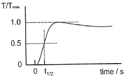
The sample temperature was measured using a Pt-13%Rh/Pt (R-type) thermocouple positioned in an alumina tube and placed close to the sample holder. In the laser flash technique, the topside of a small disc of material is irradiated with a laser, which provides an instantaneous energy pulse. The laser energy is absorbed on the top surface of a sample and gets converted to heat energy. The thermal energy is conducted through the sample. The temperature rise at the back surface of the sample is monitored using an infrared detector. A plot of the back surface temperature against time is plotted in Figure 2. The magnitude of the temperature rise and the amount of laser energy are not required for a thermal diffusivity determination, but only the shape of the curve, which is used in the analysis. The time required for the rear surface to reach half of the maximum temperature rise is denoted as t1/2. Depending on the specimen and the thermal diffusivity

value, t1/2 can range from a few milliseconds to a few seconds. The thermal diffusivity

can be expressed as: α=1.37L2/π2t1/2. Where L is the sample thickness[12].

Figure 2. The recorded temperature history at the rare surface of a specimen calculated by instrument.

Discs having 10-14 mm in diameter and approximately 2-4 mm in thickness were machined from the solid sample bulks to fit the experimental unit. For CMSX-4 and 90Ti.6Al.4V alloys, a sapphire crucible, which is transparent to laser beam and infrared rays, was used as holder. Titanium foils was placed close to sample as a local oxygen getter in the argon gas atmosphere and, thereby protect the sample from oxidation.

For liquid alloy, the sample is sandwiched between two sapphire crucibles to get an accurate thickness as shown in Figure 3a. It can be noted that the crucibles are transparent to the laser beam as well as infrared ray.

In the case of molten mould flux, the three- layered cell arrangement was employed. The three layers are composed of the liquid sample having the form of a thin film, sandwiched between two platinum crucibles. The laser pulse is exposed on the top surface of the upper crucible and the temperature rise on the rear surface of the lower crucible is monitored as a function of time. The experiment is repeated by varying the sample thickness. Figure 3b shows the schematic of three- layered arrangement.

(a) (b)

Figure 3. (a) Sample arrangement during liquid alloy thermal diffusivity measurement, (b) Schematic diagram shown the three-layered cell arrangement in the case of liquid mould fluxes.

The measurements at high temperatures were carried out in an inert atmosphere in order to prevent chemical reactions with the atmosphere. The impurity levels in the commercial argon gas had to be brought down significantly, especially the oxygen potential. In order to lower the impurity levels in the argon gas, it was subjected to a number of purification steps. The gas cleaning system used in the present work is schematically presented in Figure 4. The moisture impurity in the argon gas was removed by passing the gas successfully through silica gel as well as Mg (ClO4) 2.To remove traces of CO2 in the gas,

a column of ascarite was introduced in the gas-cleaning system. The gas was passed through columns of copper and magnesium turnings kept at 923 K and 723 K respectively [13]. The final partial pressure of oxygen in the argon purified in this way was found by using a ZrO2-CaO oxygen sensor to be less than 10-13 Pa.

Figure 4. The gas cleaning system.

2.1.2 X-ray diffraction technique

X-ray diffractometer, Philips X-pert system at the Royal Institute of Technology KTH, Stockholm, Sweden was used in the present work. The sample, either milled coke or mould slag sample, was placed on the platinum strip, which could also be used as a heater. Scattering intensities from copper Kα (wavelength λ is 1.54 Å) were used (50 kV, 40 mA) for the diffraction studies.

For coke study, it was found by preliminary trials that the typical reflection angle 2θ of the crystalline graphite (002) is 26o, which was most appropriate for monitoring the graphitisation reaction [14]. The samples were scanned over peak (002) in the scanning range (20-30)o in steps of 0.02o. Isothermal measurements were carried out at 973, 1073, 1173, 1273, 1373 and 1473 K in order to investigate the effect of the time and temperature on the degree of graphitisation.

In the case of mould flux, X-ray diffraction studies were carried out for the glassy and crystalline samples in order to determine the phase and the degree of crystallisation. X-ray diffraction profiles of crystalline samples have shown that the component can be cuspidine (Ca4Si2O7F2) or nepheline (Na3KAl4O16- NaAlSiO4). Because the largest peak

of Mn2O3 at 2θ= 32.951o does not overlap with any crystalline peaks of the sample and

the largest peak of cuspidine at 2θ=29.150o does not overlap with any of the peaks of Mn2O3, the degree of crystallisation was defined as the ratio of the largest peak intensity

of the cuspidine to that of Mn2O3 observed for X-ray diffraction profile of the well-mixed

powder of 1g of samples and 0.15 g of Mn2O3.

2.1.3 Calorimetric technique

An illustration of the NETZCH STA 449C Jupiter unit used in the present work is presented in Figure 5. The apparatus was calibrated against In, Sn, Zn, Ag and Au.

Fusion temperature and heats of fusion were in agreement with the literature [15]. The

DSC measurements were initiated by placing the CMSX-4 alloy into a platinum crucible

closed with a platinum lid [16] or milled sample of the coke into an alumina crucible

closed with an alumina lid and positioned, along with a reference with similar size specifications, on the platinum sample holder provided with a previously calibrated type S (Pt-10%Rh/Pt) thermocouple. Both crucibles were weighed before and after each DSC measurement and placed in exactly the same position throughout the measurement series. Before the experiment was started, the furnace chamber was repeatedly evacuated and flushed with purified 99.99999% Ar three times.

The DSC measurement was conducted in the temperature range of 300- 1573 K with a rate of 10 K/min in heating and cooling cycles. An initiating stabilising level at 313 K was used before the commencement of the temperature program. For a standard reference, sapphire was employed.

Gas outlet

Heating element Sample carrier Radiation shield

2.2. Materials and samples preparation 2.2.1. Alloys

CMSX-4 nickel base super alloy and 90Ti.6Al.4V alloy used in present work were supplied by Doncasters Precision Castings, Bochum GmbH, Germany. 25Cr:6Ni stainless steel was supplied by AB Sandvik Steel, Sweden and 0.7% carbon steel was supplied by CORUS Steel, The Netherlands. The chemical compositions of the alloys are presented in Table I [17].

Table

I.

Chemical compositions in mass % (except for O and S which are in ppm) of the alloys used in present work [17].

Alloy Composition

CMSX-4 Ni 60.5, Al 5.6, C 0.004, Cr 6.4, Fe 0.04, Mo 0.61, Re 2.9, Si 0.4, Ti 1.05, Ta 6.5, W 6.4, O 2*, S 2*

Ti alloy Ti 90, Al 6, V 4

Stainless steel Fe, 62.82, C 0.014, Si 0.38, Mn 0.48, Cr 25.61, Ni 6.49 Mo 3.95, N 0.252

Steel Fe 97.81, C 0.71, Si 0.35, Mn 1.09, P 0.011, S 0.02, N 0.0044, O 0.0008 * indicates ppm

2.2.2 Composite material

The composite samples used in the present work are prepared using powder sample of stainless steel AISI 304 ( Cr 17-20%, Mn < 2%, Ni 8-11%, C < 0.08%, Fe balance) with particle size less than 40 µm and aluminum oxide powder with particle size less than 10 µm. Well-mixed composite stainless steel- alumina samples with (0.001, 0.01, 0.1, 1, 2, 3, 5, 7, 8 and 10 wt %) Al2O3 were pressed into pellets using piston-cylinder die and

hydraulic press of 12 mm in diameter.

The amount of the mixture used was 3 g and the compaction pressure was about 1900 Mpa. The pressed samples were sintered at 1673 K for 20 hours using vertical furnace equipped with super Kanthel heating elements. The densities of the samples were

calculated using weight and volume and were found to be 98.5-99% of the theoretical density of the same composition.

2.2.3 Mould powder

The chemical compositions of the four proprietary mould powders used in Swedish steel industry are given in Table II. The mould powders were decarburised by heating in air for 48 h at 1073 K. The decarburised powders were placed in platinum crucibles and melted in air for 0.25 h at 1623 K for powder A, and at 1573 K for powders B-D. Glassy samples were prepared by pouring the melts onto a stainless steel plate kept at 773 K. Subsequently, the samples were annealed in air for 1h at 773 K and cooled down at the furnace-cooling rate to eliminate the residual stresses. Discs having about 12 mm in diameter and 1.5 to 2.5 mm in thickness were machined from the glassy samples. Annealing of the glassy samples having the disc shape at 1073 and 1173 K for 1-120 h led to their crystalline structure. Since the surfaces of the annealed samples became very rough because of the crystallisation, the surfaces were polished to obtain the parallelism between both faces.

Table

II

. Chemical compositions of the proprietary mould powders (mass%).

A B C D SiO2 25.5 32.7 34.2 28.8 CaO 22.7 28.8 29.4 36.5 MgO 0.97 1.77 1.01 1.3 Al2O3 12 4.7 3.92 6.5 TiO2 0.46 0.11 0.1 0.3 Fe2O3 2.86 1.24 1.09 0.8 MnO 0.04 < 0.10 0.05 3.3 Na2O 2.62 11.3 12.8 7.2 K2O 1.43 0.31 0.37 0.1 F 4.42 9.4 7.95 5.9

2.2.4 Coke

The sampling scheme of coke taken out from the Experimental Blast Furnace EBF at MEFOS Luleå, Sweden is schematically depicted in Figure 6. Coke sampling was carried out after nitrogen quenching followed by a carefully documented dissection, where approximately 20-35 pieces were taken out at different radial locations and different levels. The samples (approximately 6-8 cm3) used in the present investigation are denoted as KL05, KL10, Kl 15, KL25, and KL35. The distance (mm) of the levels KL05, KL25 and KL35 from the top are about 3961, 6652 and 6981 mm respectively. At each level, coke samples were taken from the centre (C), the place just beside the wall ( R ) and in between (M).

Figure 6. Schematic diagram of the experimental blast furnace [6].

A chemical analysis of the samples from the quenched pilot blast furnace is presented in Table III. Pellets having 10 mm in diameter and approximately 3 mm in thickness were machined from coke lumps to fit the experimental unit specification.

Table

III

. Chemical analysis in wt% of coke samples from the experimental blast furnace [6].

3. RESULTS AND DISCUSSION

Thermal diffusivity measurements of four different industrially systems, viz, metallic alloys, metallic matrix composites, mould fluxes and coke have been carried out in the present work. The influences of microstructure, phase compositions, temperature and the thermal history of these systems have been studied in present work.

XRD measurements were carried out to investigate the effect of time, temperature and chemical composition on the graphitisation phenomenon of coke using in the blast furnace. Furthermore, XRD analysis was employed in order to determine the crystallisation degree of the mould flux as a function of annealing temperature and time. The effect of crystallisation degree as well as temperature on the thermal diffusivity of mould flux has been carried out.

Heat capacity measurements of coke and CMSX-4 nickel base alloy have been carried out. Furthermore, microstructural investigations of some of these systems using Scanning Electron Microscope (SEM) equipped with Electron Dispersion Spectroscopy (EDS) also were investigated.

The following sections describe the results of the above mentioned measurements and a discussion of the same.

3.1 Thermal diffusivity measurements of alloys

3.1.1 CMSX-4 nickel base alloy

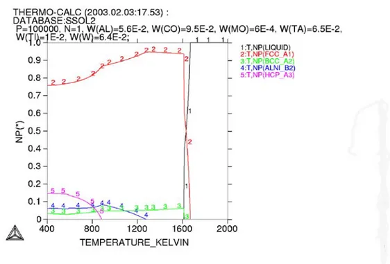
Figure 7 shows the phase diagram of an alloy close to that of CMSX-4 nickel base alloy used in the present work calculated using Thermo-calc software. For the sake of simplicity, Ti (1.05 wt%) was not taken into account in these calculations. It can be seen that the material contains fcc+bcc+hcp+Ni3Al (γ’phase) at the temperature below 1273 K.

In the presence of Ti, corresponding Ti-containing phases could be expected. Above this temperature, only fcc+bcc phases are stable and the γ’phase starts dissolving in significant amounts into the metal matrix. According to Figure 7, the solidus temperature is 1609 K and liquidus temperature is 1670 K.

Figure 7. Calculated phase diagram of an alloy with composition close to the present CMSX-4 alloy using Thermo-calc software.

In Figure 8, all the experimental results of the thermal diffusivity measurements with as received alloy samples are presented as functions of temperature. It can be seen that the thermal diffusivity increases with temperature up to 1223 K. Above this temperature, the diffusivity shows a slight decrease and/or become constant. In the solid-liquid zone, it is difficult to observe any definite trend as the experimental scatter is significant. In fact, above 1223 K, different experimental runs give varying results, which could be due to the thermal history of the industry sample received.

0 200 400 600 800 1000 1200 1400 1600 0,020 0,025 0,030 0,035 0,040 0,045 0,050 0,055 0,060 0,065 fcc+bcc fcc+bcc+Ni₃Al fcc+bcc+Ni₃Al+hcp Solidus temp. Liquidus temp. Equilibrium values Heatng1 Cooling1 Heating2 Cooling2 Heating3 Cooling3 Heating4 Cooling5 Thermal Di ffusi vi ty cm 2 /s Temperature K

Figure 8. Thermal diffusivity-temperature curves of CMSX-4 alloy including the equilibrium values.

Figure 8 shows also that there is no significant change in the thermal diffusivity values after annealing during isothermal measurements (cooling 5) at 1277, 1403 and 1531 K as a function of time or temperature and that the values obtained after annealing are lower than those measured without annealing treatment. This is indicative of the attainment of thermodynamic equilibrium, where the dissolution of the intermediate phases in the matrix might have been completed and the attainment of impurity levels in the matrix was in maximum.

The thermal conductivities of the CMSX-4 alloy were calculated from experimental thermal diffusivities using the values of the specific heat and density according to the formula

κ= α. Cp.ρ (1)

where “κ” is the thermal conductivity W.m-1_.K-1_{, “α”, the thermal diffusivity m}2_.s-1_{, “C} p”,

the heat capacity J.Kg-1.K-1 and “ρ” the density Kg.m-3_.

The heat capacity and density values of the alloys investigated in the present work have been reported by [16] and [17] respectively. For the above calculations, the average values of thermal diffusivities from Figure 8 were used. The thermal conductivities calculated from above formula can be shown in Figure 9.

200 400 600 800 1000 1200 1400 1600 1800 6 8 10 12 14 16 18 20 22 24 26 Ther mal C ond ucti vity (κ ) , W. m -1 .k -1 Temperature (K)

Figure 9. The Thermal conductivity of CMSX-4 alloy with respect to temperature.

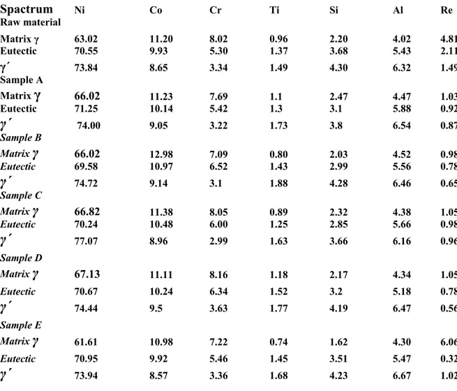
For structure studies of this alloy, samples A and B were heated to 600 and 1000 K, respectively, at the rate of 6 K/min and subsequently quenched into water. Samples C and D were heated to 1573 K at first, then cooled to 600 and 1000 K, respectively, at the rate of 6 K/min, and then quenched into water in order to determine the effect of microstructure of the alloy on the temperature dependence of the thermal diffusivity. On the other hand, sample E was heat-treated at 1373 K for 30 minutes and quenched in water. Figure 10 shows the microstructure of the heat treated samples (A-E) as well as received sample. Table IV shows the phase composition of these samples using EDS attached to SEM.

The thermal diffusivity measurements of samples A-E, quenched from different temperatures show almost same value. This value is close to the thermal diffusivity of the raw sample at room temperature.

C E Euutteeccttiiccssttrruuccttuurree Gamma D A E Euutteeccttiiccssttrruuccttuurree Gamma γ’ E Euutteeccttiiccssttrruuccttuurree γ’ Gamma Raw material E Gamma E Euutteeccttiicc γ’ γ’ γ’ E Euutteeccttiicc ssttrruuccttuurree Gamma B E Euutteeccttiic cssttrruuccttuurree γ’ Gamma

Figure 10. SEM pictures of annealed CMSX-4 alloy during: A,B) quenched from 600, 1000 K, C,D) quenched samples after heating to 1573 and cooling down 600 and 1000 K, E) heat treated sample at 1373 K for 30 minutes and quenched in water and raw material.

Table IV. Main chemical composition wt% of annealed CMSX-4 samples A-D using Spactrum Ni Co Cr Ti Si Al Re l 3.02 1.20 .02 0.96 2.20 .02 .81 ple A 6.02 1.23 7.69 .1 .47 .47 .03 ple B 6.02 2.98 .09 0.80 2.03 .52 .98 ple C 6.82 1.38 .05 0.89 2.32 .38 .05 ple D 7.13 1.11 .16 1.18 2.17 .34 .05 ple E 1.61 0.98 .22 0.74 1.62 .30 .06

EDS attached to SEM.

Raw materia Matrix γ 6 1 8 4 4 Eutectic 70.55 9.93 5.30 1.37 3.68 5.43 2.11 γ´ 73.84 8.65 3.34 1.49 4.30 6.32 1.49 Sam Matrix

γ

6 1 1 2 4 1 Eutectic 71.25 10.14 5.42 1.3 3.1 5.88 0.92

γ´

74.00 9.05 3.22 1.73 3.8 6.54 0.87 Sam Matrix

γ

6 1 7 4 0 Eutectic 69.58 10.97 6.52 1.43 2.99 5.56 0.78

γ´

74.72 9.14 3.1 1.88 4.28 6.46 0.65 Sam Matrix

γ

6 1 8 4 1 Eutectic 70.24 10.48 6.00 1.25 2.85 5.66 0.98

γ´

77.07 8.96 2.99 1.63 3.66 6.16 0.96 Sam Matrix

γ

6 1 8 4 1 Eutectic 70.67 10.24 6.34 1.52 3.2 5.18 0.78

γ´

74.44 9.5 3.63 1.77 4.19 6.47 0.56 Sam Matrix

γ

6 1 7 4 6 Eutectic 70.95 9.92 5.46 1.45 3.51 5.47 0.32

γ´

73.94 8.57 3.36 1.68 4.23 6.67 1.02

The thermal conductivity,κ, can be considered to be due to electron or lattice vibrations, the latter even referred to as phonon conduction. According to Debye [18], the thermal diffusivity can be expressed by the equation:

vl nCv 3 1 = κ (2)

where n is the number of particles per unit volume, CV is the heat capacity at constant

volume per particle (so that nCv is the heat capacity per unit volume expressed in J.K.m-3),

the velocity of sound and l is the mean free path [19, 20]. Assuming that the velocity

of sound is constant, the thermal conductivity will be proportional to electrons or phonons mean free path. The term l is dependent on collision between electrons or

phonons as well as with lattice defects.

v

v

The thermal diffusivity measurements of samples A-D, quenched from different temperatures show almost same value. This value is close to the thermal diffusivity of the raw sample at room temperature. It can be observed that the positive temperature dependence of thermal diffusivity shown in Figure 8 is independent of microstructure below 1223 K. The thermal conductivity in Figure 9 was found to increase with temperature and can be considered as proportional to Tn. If l is independent of T, the

thermal conductivity will be proportional to CV, which, in turn, is approximately

proportional to T3 [20]. The situation in the present case is complicated due to the industrial sample being investigated, where the precipitation of intermediate phases like Ni3Al (γ´ phase) might not have reached equilibrium state.

At later stages, in the temperature range 1223 K to solidus temperature, the thermal diffusivity in Figure 8 as well as the thermal conductivity in Figure 9 show constancy or a slight decrease with temperature. This could be that, in this range of temperatures, the intermediate phases, which have nucleated, started to dissolve in the matrix. The variation of thermal diffusivity/conductivity with temperature can be attributed to a) in the presence of γ´ phase, the electrical resistivities increased and as a result the thermal conductivity decreased. On the other hand, the coarsening of this phase by increasing temperature causes decreasing of electrical resistivity and as a result, increasing of the thermal conductivity [21]. At this temperature range, the mixing of these two mechanisms can cause the constancy or a slight decreasing of thermal conductivity b) as the impurity level in the matrix increases due to the dissolution γ´ phases, the disorder of the alloy increases, the mean free path decreases c) part of the heat energy supplied by the laser shot is absorbed at phase transformation viz. the dissolution of γ´ phase. Figure 8 shows that there is no significant change in the thermal diffusivity values after annealing during isothermal measurements at 1277, 1403 and 1531 K as a function of time or temperature and that the values obtained after annealing are lower than those measured without annealing treatment. This is indicative of the attainment of thermodynamic equilibrium, where the dissolution of the intermediate phases in the matrix might have been complete and the attainment of impurity levels in the matrix was in maximum.

In liquid state, the average value was 0.058 cm2/s and it can be seen that there is no significant change with increasing temperature. It may be attributed to the decrease of the mean free path being shorter than characteristic distance between two neighboring atoms. It is admitted that the present thermal diffusivity values in liquid state could be affected by a certain degree of convection (the upper liquid surface was 2 K higher than the bottom and thus the convective force has to work against gravity) as well as the free liquid surface between the crucibles, which was about 12% of the total sample surface as shown in Figure 11. 1760 1780 1800 1820 1840 1860 0,030 0,035 0,040 0,045 0,050 0,055 0,060 0,065 0,070 0,075 0,080 Th e rm a l d iffu sivity cm 2 /s Temperature K Figure 11. Results of Thermal diffusivity measurements in the case of liquid CMSX-4 alloy.

3.1.2. 90Ti.6Al.4V alloy

Thermodynamic stabilities of this alloy under investigation at various temperatures were carried out with the help of Thermo Calc software. Figure 12 shows the phase diagram of the alloy used in the present work, computed using this software. It can be seen that the material contains bcc+hcp+Ti3Al (γ’ phase) at temperatures below 1203 K. Above

this temperature, only bcc phase is stable and the γ’phase dissolves into the metal matrix. According to Figure 12, the solidus temperature is 1965 K and liquidus temperature is 1971 K.

Figure 12. Calculated phase diagram of 90Ti.6Al.4V alloy.

During the thermal diffusivity measurement of 90Ti.6Al.4V alloy, the samples were heated to 1673 K and cooled to room temperature at the rate of 6 K.min-1. Microscopic observations showed that the sample surface was found to be rough after the annealing at high temperatures owing to the grain growth. Consequently, it was considered that the data obtained during the cooling cycle were not reliable and ignored in trials 1, 2 and 3. In order to study the effect of the thermal history of the alloy, in trial 4, the sample was kept at 1650 K for 11h, cooled in the furnace and polished to make the surface smooth. In this particular case, the thermal diffusivity measurements were carried out during heating and cooling cycles.

Figure 13 shows the experimental results of the thermal diffusivity measurements as a function of temperature of 90Ti.6Al.4V. The stability regions of the various phases in the 90Ti.6Al.4V have been presented along with the thermal diffusivity values in this figure. It is seen that the thermal diffusivity increases with temperature below 1225 K. This might be due to the fact that the mean free path might be increasing with temperature. It can also be observed that the sample annealed at 1649 K for 11 hours (sample 4) has lower thermal diffusivity compared to the non annealed samples. This difference is attributed to the difference in the annealing history of the sample. A slight decreasing and/or constancy of thermal diffusivity was observed above 1223 K. In this region, the intermediate phase, Ti3Al, dissolves in the matrix to varying extents causing an increase

200 400 600 800 1000 1200 1400 1600 1800 0,00 0,02 0,04 0,06 0,08 0,10 0,12

* Sample heat treated at 1649 K for 11 hours

bcc hcp+bcc hcp+bcc+Ti₃Al Heating1 Heating2 Heating3 Heating4* Cooling4* Therm a l D iffus iv ity c m 2 .s -1 Temperature, K

Figure 13. Thermal diffusivity- temperature curves of 90Ti.6Al.4V alloy.

The estimated thermal conductivities using equation (1) of 90Ti.6Al.4V alloy were calculated from the present results and the literature values of Cp and ρ [22]. The thermal conductivity as a function of temperature was plotted in Figure 14.

Mills [22] has earlier presented a model for estimating the thermal conductivity of titanium alloys using the following equations:

298 ≤ T ≤ 973 K: κT = κ298 +(23-κ298) * (T-298)/657 (3)

973 ≤ T ≤ 1273: κT = 15.2+0.0273 (T-973) (4)

1273 ≤ T ≤ 1923: κT = 23 + 0.0075 (T- 1273) (5)

In order to use the equations, it is necessary to incorporate the values for the thermal conductivity at room temperature. In the present calculations, the results obtained at room temperature in this work were used. The experimental results obtained are compared with those obtained by using Mills equation in Figure 14.

In this case, the agreement with the experimental values is satisfactory in the entire temperature range of the measurements. Thermal conductivity values of the pure components reported by [22] and [23] have also been shown in same figure for comparison. It is seen that the thermal conductivity values are very close to those of pure Ti.

0 200 400 600 800 1000 1200 1400 1600 1800 0 50 100 150 200 250 Pure Titanium (22) Pure Venadium (23) Pure Aluminium (22) 90Ti.6Al.4V Alloy present work

Mills model using present experemental value at room temp.

T herm al co nduct ivit y K , W. m -1 .K -1 Temperature, K

Figure 14. Thermal conductivity of 90Ti. 6Al. 4V alloy compared with thermal conductivity calculated by Mills model using the experimental value at room temperature as a start value.

3.1.3. 25Cr:6Ni stainless steel

Figure 15 shows the computed phase diagram of stainless steel alloy. It can be seen that the material contains bcc + fcc+ σ below 928 K. Between 928 and 1171 K, fcc and σ phases are stable and fcc + bcc phases are stable between 1171 K and solidus temperature, which is 1615 K. Thus, the σ phase (FeCr) is stable in the temperature interval between room temperature and 1218 K. The liquidus temperature is 1717 K.

Figure 15. Calculated phase diagram of 25Cr:6Ni stainless steel.

Figure 16 shows the temperature dependence of the thermal diffusivity of stainless steel sample. The phases predicted by the thermodynamic computation are marked in the figure as well. It can be seen that the thermal diffusivity is nearly constant up to about 700 K. Beyond this temperature, there is an increase of the thermal diffusivity with increasing temperature. These results are in agreement with that of AISI 301 and AISI 304 austenitic stainless steel, which are nonmagnetic materials [24]. The data obtained during the cooling cycle is almost identical to that during heating cycle. It means that the effect of σ phase on the thermal diffusivity is negligible in this temperature range. The increase in the slope of the curve above 950 K can be due to increase in the bcc portion in the structure.

200 400 600 800 1000 1200 1400 0,030 0,035 0,040 0,045 0,050 0,055 0,060 0,065 0,070 0,075 σ phase bcc+fcc fcc bcc+fcc

Heating (Experimental value) Cooling (Experimental value) Litreture value (AISI 301)24 Litreture value (AISI 304)24

Thermal D iffus iv ity c m 2 .s -1 Temperature, K

Figure 16. Thermal diffusivity-temperature curves of stainless steel.

The estimated thermal conductivities of 25Cr:6Ni stainless steel based on equation (1) were found to be in good agreement with the thermal conductivity of the same alloy used Mills model, which used equations (6) and (7) to determine the thermal conductivity of steel. This agreement can be seen clearly in Figure 17. It should be pointed out that the experimental thermal conductivity value at room temperature obtained in the present investigation was used as a start value of Mills model.

298 ≤ T ≤ 1073 K: κT =κ298 + (25-κ298) * (T-298)/775 (6)

200 400 600 800 1000 1200 1400 1600 15 20 25 30 35 40 45 50 Present work

Mills model using the present experimental value at room temperature as a start value

Th er mal conducti vity K, W .m -1 .K -1 Temperature, K

Figure 17. Thermal conductivity of stainless steel compared with thermal conductivity calculated by Mills model using the experimental value at room temperature as a start value.

3.1.4. 0.7% carbon steel

Figure 18 shows the phase diagram of high carbon steel used in present work. It can be seen that the material contains bcc phase at temperature below 954 K. Between 954 and 1026 K bcc + fcc phases are stable. Above this temperature, fcc phase is stable until the solidus temperature, which is 1638 K. The figure also shows that the liquidus temperature is 1746 K.

Figure 18. Calculated phase diagram of 0.7%C Steel.

Figure 19 shows the thermal diffusivity measurement results obtained in the case of 0.7% carbon steel as a function of temperature. The figure shows that the thermal diffusivity of the plain carbon steel sample decreases with increasing temperature where the microstructure contains bcc phase. The corresponding values for Armco iron, taken from literature [25] show a similar trend. The minimum thermal diffusivity values can be observed at 970 K (Curie point). If a ferromagnetic transition exists in a metal, thermal diffusivity always decreases from room temperature to the Curie temperature, as the disorder increases [25,26,27]. Beyond this point, thermal diffusivity shows an increase.

0 200 400 600 800 1000 1200 0,02 0,03 0,04 0,05 0,06 0,07 0,08 0,09 0,10 0,11 0,12 0,13 0,14 fcc bcc+fcc bcc

....:Literature value(Armco iron)25 Heating (Experimental value) Cooling (Experimental value)

T h e rm a Diffus ivity c m 2 .s -1 Temperature, K

Figure19. Thermal diffusivity-temperature curves of 0.7% carbon steel.

The estimated thermal conductivity of 0.7% carbon steel based to equation (1) was found to be in good agreement with the thermal conductivity of the same steel used Mills model, obtained from equations (6) and (7) using the present experimental thermal conductivity value at room temperature used as a start value of Mills model. This agreement can be seen clearly in Figure 20.

200 400 600 800 1000 1200 1400 1600 20 30 40 50 60 70 80 90 100 _{Present work}

M ills m odel using present experim ental value at room tem perature as start value

Thermal c o nductivit y k , W .m -1 .K -1 Tem perature, K

Figure 20. Thermal conductivity of 0.7% carbon steel alloy compared with thermal conductivity calculated by Mills model using the present experimental value at room temperature as a start value.

3.1.5. Electron contribution of thermal conduction of alloys

The thermal conductivity of the metals and alloys is composed of two components: a lattice component

k

g and electronic component

k

e.In both cases, heat is transported by mobile carriers. Weidman-Franz-Lorenz formula has been used to calculate the thermal conductivity using electrical resistivities of the alloys similar in composition to the above-mentioned alloys at room temperature [21, 28]. The aim of this calculation is to estimate the contribution of the electron as heat conductor in these alloys. The relevant equation is

κ/ σ

e

.T

= 2.45*10-8 W.Ω.K-2 (8)

Where

κ

is the thermal conductivity W.m-1.K-1, σe is the electrical conductivity Ω-1. m-1

and T is the absolute temperature (Kelvin). Table V shows the calculated and measured thermal conductivity of above mentioned alloys.

Table V.Calculated electrical conductivity and measured thermal conductivity of alloys used in present work.

Material

Electrical

conductivity

Ohm

-1

.m

-1

Calculated

thermal

conductivity

W.m

-1

.K

-1

Measured

thermal

conductivity

W.m

-1

.K

-1

Electron

contribution %

CMSX-4 65.13*10

4

4.755 7.807 61

90Ti.6Al.4V 50.7*10

4

3.7 6.68 55.4

25Cr:6Ni

stainless

steel

86.2*10

4

6.3 14.55

43.3

0.7% carbon

steel

57.4*10

5

41.9 42.50 98.6

It can be seen that the addition of Cr to the steel decreases the electronic contribution from 98.6% to 43.3%. On the other hand, the presence of Ti3Al in the titanium alloy as

well as Ni3Al in CMSX-4 alloy cause a lowering of the electrical conductivity as well as

electron contribution to the thermal conductivity of these alloys. The electrical conductivity of pure nickel and titanium are 125 *105 and 180*104 respectively [28].

3.2. Composites

Compositions of various AISI 304 Stainless steel- alumina composites used in this study and their densities, ρ, are presented in Table VI. It can be seen that the density of the specimens decreases with increasing the alumina content.

Table VI. Densities of AISI 304 stainless steel-alumina composites.

Sample SSxx* Reference SS0 SS0.001 SS0.01 SS0.1 SS1 SS2 SS3 SS5 SS7 SS8 SS10 Density kg/m3 *103 7.6 7.54 7.58 7.57 7.51 7.43 7.43 7.29 7.18 7.12 6.639 6.609

* The number beside SS refers to the Al2O3 wt% content in the sample composition. Typical SEM micrographs taken from polished cross-sections of Stainless steel-alumina composites are shown in Figure 21. It can be seen that the alumina particles are uniformly dispersed through the material at low alumina contents. No appreciable deformation or microcracks of adjoining grains in the composites, which might occur due to thermoelastic mismatch between the stainless steel and the alumina particles, could be detected. At higher alumina contents, a tendency of alumina particles to agglomerate is evident.

SS0 SS0.001 SS0.01

SS0.1 SS1 SS2

SS3 SS5 _SS7

Figure 21. SEM micrograph of polished cross-sections of AISI 304 Stainless steel-alumina composite containing various steel-alumina wt%.

Thermal diffusivities of cold pressed and sintered specimens of AISI 304 stainless steel-alumina composites of various compositions, as a function of temperature, are shown in Figure 22.

200 400 600 800 1000 1200 1400 0,03 0,04 0,05 0,06 0,07 ss 0 ss 0.001 ss 0.01 ss 0.1 ss 1 ss 2 ss 3 ss 5 ss 7 ss 8 ss 10 T hermal di ff us ivi ty u cm 2 /s Temperature K

Figure22.Temperature dependence of thermal diffusivity of Stainless steel-alumina composite containing (0-10) wt% alumina.

The thermal conductivities of the specimens, investigated in the present work could be calculated using simple rule of mixture at every temperature from experimental thermal diffusivities, the values of the heat capacity reported by [29] and density according to equation (1). The thermal conductivities thus computed are presented in Figure 23. It can be seen that the thermal diffusivity as well as thermal conductivity of specimens increase with the temperature as shown in Figures 22 and 23. This tendency could be due to increase of the electron-electron mean free path with increasing temperature. These results are in agreement with that of austenitic stainless steel, which is a nonmagnetic material as reported by Westover [30]. Figure 23 also shows that there is no significant change of the thermal conductivity with increasing alumina content in the range between 0 and 5 wt% alumina. Above that, the thermal conductivity decreases with increasing the alumina content. This trend is clearer at high temperatures. At lower temperatures, the combination of the two opposing effects, viz, decrease in the thermal conductivity due to increase of alumina content, which is an insulator to the electron transport and the increase due to increase in the thermal conductivity of alumina itself might be plausible reasons.

200 400 600 800 1000 1200 1400 15 20 25 30 35 ss 0 ss 0.001 ss o.o1 ss 0.1 ss 1 ss 2 ss 3 ss 5 ss 7 ss 8 ss 10 T h er m a l C o n d u c ti v ity W .m -1 .K -1 Temperature K

Figure 23. Temperature dependence of thermal conductivity of Stainless steel-alumina composite containing (0-10) wt% alumina.

The thermal conductivity as a function of the alumina content at 970 and 1162 K is plotted in Figures 24 and 25 respectively. No evidence of difference between the trends of the values between these two figures could be noted. This might be due to the same behavior of the electrons transport at these temperatures.

In this study, simple rule of mixture reported by James et al [31], Eucken equation reported by Hayashi et al [32], and Ohm´s law model developed by Hayashi et al [33] have been used to compare the measured values with these models as shown in Figures 24 and 25.

0,90 0,92 0,94 0,96 0,98 1,00 0 10 20 30 40 50 T= 970 K Present work Hayashi et al (33) model

Simple rule of mixture model(31)

Eucken equation (32) Ther mal conduc tivity K e , W .m -1 .K -1 Purity (1- Al₂O₃%)

Figure 24. Effect of the alumina content on the thermal conductivity of stainless steel-alumina composite at 970 K compared to previous models.

0,90 0,92 0,94 0,96 0,98 1,00 0 10 20 30 40 50 T=1162 K Present work Hayashi et al (33) model

Simple rule of mixture model(31)

Eucken equation (32) The rm al c ond uc tivity Ke , W. m -1 .K -1 Purity (1-Al₂O₃%)

Figure 25. Effect of the alumina content on the thermal conductivity of stainless steel-alumina composite at 1162 K compared to the previous models.

In the simple rule of mixture, the thermal conductivity of the composites (κc)can be

written as follows:

κc=(κst.st * χst.st) + (κAl2O3 * χAl2O3) (9)

where κc,κst.st andκAl2O3 represent the thermal conductivity of composites, stainless

steel and alumina respectively and χst.st , χAl2O3 are the weight fraction of stainless steel

and alumina.

On the other hand, the thermal conductivity of a binary phase material κc generally

obeys the Eucken relationship, when a minor amount of discontinuous second phase disperses uniformly in a continuous phase. Eucken equations are:

) . 1 ( ) . 2 1 ( 3 2 3 2 . A A Kc O Al O Al st st φ φ κ − + = (10) where ØAl2O3 is the weight fraction of alumina and

1 ) / 2 ( ) / ( 1 3 2 . 3 2 . + − = O Al st st O Al st st k K k A κ (11)

Furthermore, The Ohm´s law model developed by Hayashi et al, introduces the finite transverse heat flow, i.e., in X and Y direction as shown in Figure 26.

R5

R4

R3

R2

R1

0

V

V1

V2

Figure 26. Simple Ohm´s law model including the finite transverse heat flow [33].

This model considers that the effective thermal conductivity Kc of the composites corresponding to the reciprocal of the five-resistor circuit. The value of Kc can be written by applying Ohm´s law:

Kc=(V1/R4 +V2/R5) (12) here the value of R1,R2,R3,R4 and R5 can be written as follows:

R1=(1-L)/(AKS) (13)

R2=(1-L)/((1-A)Ks) (14) R3=1/[4(1-L)Ks] (15) R4=L/(AKf) (16) R5=L/((1-A)Ks) (17)

where L and A are the length and the cross/ section area of a rectangular alumina particle, respectively. Ks and Kf are the thermal conductivity of the matrix and alumina particles

respectively.

The Potentials V1 and V2 in the equation (12) and Figure 26 can be expressed using Kirchhoff´s law as follows:

) 5 1 3 1 2 1 )( 4 1 3 1 1 1 ( 3 1 ) 5 1 3 1 2 1 ( 1 3 2 1 3 1 2 R R R R R R R R R R R R R VR V + + + + − + + + − = (18) ) 4 1 3 1 1 1 )( 5 1 3 1 2 1 ( 3 1 ) 4 1 3 1 1 1 ( 2 3 1 1 3 2 2 R R R R R R R R R R R R R VR V + + + + − + + + − = (19)

Figure 24 and 25 show that all the three mentioned models are almost overlapping on each other. They are also in good agreement with the present experimental values, when the weight fraction of the alumina is lower than 5wt%. Above this ratio, there large discrepancy can be observed. This discrepancy could be due to the agglomeration of the alumina particles during pressing and sintering. This agglomeration may cause the “leak away” and scattering of the electrons during heat transport, which decreased the thermal conductivity of the composites. Such agglomeration can be seen in Figure 21.

3.3. Mould powder

3.3.1. XRD measurements

X-ray diffraction profiles of all glassy samples indicate no traces of crystalline phases, indicating that all glassy samples are amorphous from the viewpoint of x-ray diffraction. Figure 27 shows the x-ray diffraction profiles of the glassy sample (a) and the samples annealed at 1073 K for 1 h (b) and 15 h(c) for powder A. It can be seen that Figure 27 (a) corresponds to the glassy structure. On the other hand, in Figure 27 (b), which corresponds to that for the sample annealed at 1073 K for 1 h, two sharp peaks appear together with the hallow pattern due to the amorphous phase. Two sharp peaks may be attributed to nepheline (Na3KAl4Si4O16, NaAlSiO4). On the other hand, Figure 27 (c)

shows that the hallow pattern disappears and only sharp peaks are observed for the sample annealed at 1073 K for 15 h, indicating that the sample has been mostly crystallised. Markings have been made at the angles where the diffraction peaks attributed to cuspidine (Ca4Si2O7F2) and nepheline (Na3KAl4Si4O16, NaAlSiO4) should be

observed.

Figure 27. X-ray diffraction profiles of the glassy sample(a) and the samples annealed at 1073 K for 1 h(b) and 15 h(c) for powder A.

Figure 28 shows the X-ray diffraction profiles of the samples annealed at 1073 K for 1h for powders B-D. Marking has been made at the angles where the diffraction peaks attributed to cuspidine and nepheline should be observed for powder B, and at the angles where the peaks due to cuspidine should be observed for powders C and D.

Figure 28. X-ray diffraction profiles of the samples annealed at 1073 K for 1 h for powder B-D.

3.3.2 Thermal diffusivity measurements

Figure 29 shows the temperature dependences of the thermal diffusivities of the glassy samples and the samples annealed at 1073 K for 1-120 h for powder A, 1-15 h for powder B and 1 h for powder C and D respectively. Closed symbols are data recorded during the heating cycles and open symbols during the cooling cycles.

400 600 800 1000 5 6 7 8 9 Glassy 1h 4h 15h 120h Temperature / K Thermal diffusivity / 10 -7 m 2 s -1 powder A 400 600 800 1000 4 5 6 7 8 Glassy 1h 15h Temperature / K Thermal diffusivity / 10 -7 m 2 s -1 powder B 400 600 800 4 6 8 10 12 Glassy 1h Temperature / K Thermal diffusivity / 10 -7 m 2 s -1 powder C 400 600 800 4 5 6 7 8 Glassy 1h Temperature / K Thermal diffusivity / 10 -7 m 2 s -1 powder D

Figure 29. Temperature dependencies of the thermal diffusivities of the glassy and crystalline samples for powders B, C and D, respectively.

It can be seen from these figures that the thermal diffusivities of the crystalline samples decrease with increasing temperature at lower temperatures and are roughly constant at higher temperatures. These temperature dependencies were in agreement with those reported by Shibata et al [34]. It can be also seen that the sample annealed for longer time exhibits larger thermal diffusivity in the case of powder A.

Thermal diffusivity is determined by lattice vibration (phonon conduction) in insulators. Since Cv ≈ ρCp, Eqs. (1) and (2) yield, the thermal diffusivity can be describe as the

vl

3 1 =

α (20)

If it is assumed that the value of v is constant irrespective of temperature, the thermal diffusivity is proportional to the phonon mean free path. As mentioned earlier, the phonon mean free path is determined principally by two mechanisms, geometrical scattering, i.e., the collisions of phonons with the crystal boundary, lattice imperfections and so on and phonon-phonon interaction. The reciprocal of the effective mean free path 1/l is found by adding the reciprocal of the mean free path for geometrical scattering lgeo

and that for phonon-phonon interaction lp-p, as follows;

p p geo l l l = + ₋ 1 1 1 (21)

Generally, above room temperatures, the geometrical scattering is independent of temperature. On the other hand, the mean free path, determined by phonon-phonon interaction is inversely proportional to temperature above the Debye temperature [18]. Therefore, Eq. (21) is rewritten as

bT a

l = +

1

(22)

where T is the absolute temperature and a and b constants. If the temperature is raised to a sufficiently high level, the mean free path decreases to a value near the lattice spacing, and is expected to be independent of temperature [35]. The solid lines in the figures have been drawn based on Eq. (22). Figure 30 shows the temperature dependencies of the thermal diffusivities of the glassy sample and the samples annealed for 1 h at 1073 and 1173 K for powder A.