Granger Causality Between Exports and Growth in OECD Countries : A Panel Data Approach

Granger Causality Between Exports and

Growth in OECD Countries

BACHELOR

THESIS WITHIN: Economics

NUMBER OF CREDITS: 15ETCS

PROGRAMME OF STUDY: International Economics and Policy

AUTHOR: Gabriela Markova

TUTOR: Pär Sjölander and Emma Lappi

JÖNKÖPING May 2016

Bachelor Thesis in Economics

Title: Granger Causality Between Exports and Growth in OECD Countries: A Panel Data Approach

Author: Gabriela Markova

Tutors: Pär Sjölander and Emma Lappi Date: 2016-05-23

Key words: OECD, Causality, Economic Growth, Export, Panel data

Abstract

This paper investigates the possibility of Granger causality between growth and exports, measure in logarithms of real GDP and real exports in 26 OECD countries from 1971 to 2014. A panel data approach is applied based on VAR systems and Wald tests on the panel, as well as on each individual country. Two different specifications are used: a bivariate (GDP-exports) and a trivariate augmentation including trade openness (GDP-exports-openness). The variable of trade openness is used as a specification in the trivariate model and it is expected to estimate the sensitivity of GDP and exports. The results from the cross country analysis indicate unidirectional causality from exports to GDP in Greece and Italy, one-directional causality from GDP to exports in Denmark, Germany, Korea, New Zealand, the Netherlands, Canada and Norway, bidirectional causality between exports and growth in Japan, Sweden and Turkey, while in the cases of Australia, Austria, France, Iceland, Ireland, Mexico, Spain, Switzerland and the United States there is no statistical evidence for any causal relationship. The results from the two models are ambiguous for five countries, namely Belgium, Finland, Luxembourg, Portugal and Great Britain; therefore there is not sufficient evidence in order to draw any conclusions. Nevertheless, the results from the panel analysis show a significant statistical evidence for unidirectional causality from GDP towards exports lending support to the growth-driven-export hypothesis. The conclusions from this paper show that trade has a positive effect on growth, as expected from theory and as previously found in cross-country studies.

Acknowledgements

I would like to thank my supervisor Pär Sjolander for the provided insights and

expertise during the process of writing this thesis. His commens and valuable

feedback were crusial in improving the quality of this paper.

Table of Contents

1 Introduction ... 1

1.1 Purpose ... 2

1.2 Background ... 2

1.2 Delimitations ... 3

1.3 Dispositions ... 3

2 Theoretical Background ... 4

2.1 Neoclassical Approach ... 4

2.2 Endogenous growth theory ... 4

2.3 Institutional approach ... 5

2.4 Controversial Results ... 5

2.5 Defining trade openness ... 6

2.6 Relationship between exports and economic growth ... 6

3 Data, empirical model and method ... 10

3.1 Data and variable description ... 10

3.2 Model ... 11

3.3 Method ... 13

3.3.1 Lag Length Selection ... 13

3.3.2 Unit Root test ... 14

3.3.3 Cointegration test ... 17

3.3.4 Granger causality ... 20

4 Empirical Results ... 23

5 Conclusion ... 26

Tables

Table 1. Descriptive Statistics ... 11

Table 2. VAR Lag Order Selection Criteria ... 14

Table 3. Fisher-ADF Unit Root Test ... 15

Table 4. Individual unit root tests ... 16

Table 5. Hadri test results ... 17

Table 6. Johansen Cointegration Test ... 18

Table 7. Individual Cointegration test ... 18

Table 8. Granger Causality tests ... 21

Table 9. Wald tests on the coefficients ... 22

Table 10. Wald tests for Granger-causality in the bivariate model, in first difference ... 23

Table 11. Wald tests for Granger-causality in the trivariate model, in first difference ... 24

Tabel 12. Vector Autoregressive Models ... 31

Appendix

1 Introduction

This section introduces and presents the reader to the broader overview of the topic of this paper. First, there is a preface description of the subject matter, followed by the purpose, background and delimitations.

Economic growth is one of the essential determinants of economic welfare. The relation between exports and economic growth has been frequently discussed when analysing the degree of economic prosperity among different countries. Exports represent one of the most valuable and substantial sources of foreign exchange revenue and are one of the fundamental components of international trade. This argument dates back to the classical economic theories by David Ricardo, who claimed that international trade has a major influence on economic growth. The theory of international trade is one of the earliest branches of economic ideologies. Trade policy is an essential tool in accomplishing the objective of sustained economic growth. Increased trade openness and trade liberalization has established the foundation of dynamic gains from trade. The neoclassical approach supports the concept of comparative advantage, where gains from trade arise from diverse factor endowments and technological progress. A fundamental principle of the neoliberal paradigm on globalization is the belief that increased trade openness through eradication of trade barriers is the solution to improved global prosperity.

The importance of exports in trade liberalization growth strategies has been evident since the failure of the Import-Substitution Industrialization strategy and debt crisis in the 1980s. Consequently the adoption of export promotion strategies and trade integration has taken place, with many of the developing countries instituting reforms aiming at export expansion and eliminating trade barriers. According to prevalent economic theory, lack of trade openness will deteriorate the economic growth. If a country imposes restrictive policies as high trade tariffs or quotas, this will prevent other countries in wishing to engage in international trade. These enforced barriers will obstruct trading partners in sending exports and receiving imports. In order to aid the economic development, governments impose economic policies which remove trade barriers, such as tariff rates. These measures are established under trade liberalization policies.

Due to the liberalization wave initiated in the last decades, economists have discussed the different links and causality between trade openness, economic growth and income distribution (Rodriguez and Rodrik, 2001). Policies focused on the expansion of external markets promote product development and expose domestic industries to foreign competition. Empirical research has proven that, in the long-run, more export-oriented countries have recorded improved economic growth performance. The volume of trade indicates the extent of a country’s integration in the world economy, prompting greater market opportunities and increased international competition. This leads to more efficient use of domestic resources, economies of scale, access to new technologies through foreign capital inflow and promotes innovation. A prominent example in support of the success of these theories is the remarkable economic growth and rapid industrialization exhibited by the four East Asian Tiger economies (South Korea, Singapore, and Hong-Kong, Taiwan).

During the post liberalization period, the role of exports on the economic prosperity in developing countries has become a widely researched topic. Exports can assist in the integration process of countries in the international market and diminish the effect of external shocks on the domestic economy. Systems which stimulate export expansion have exhibited improved economic growth by inducing positive externalities through means of specialization, efficient resource allocation, improved production capacity, scale economies, increased capital formation and domestic production through import of capital and intermediate goods. Through the revenue generated from exports, developing countries have the opportunity to import capital equipment and raw materials which are further contributing to the economic progress.

1.1 Purpose

The purpose of this paper is to study the possibility of Granger causality between real exports and real GDP and examine the causality direction in twenty six OECD1 _{countries during the}

period of 1971-2014. The relationship is empirically investigated by applying a bivariate (GDP-Exports) model and a trivariate (GDP-Exports-Openness) model and focuses on examining one-period-ahead causality. Granger Causality econometric technique will be tested in an unrestricted VAR model to show if exports are Granger causing economic growth, or vice versa. The approach of testing the causal relationship using a panel data approach is inspired by an earlier study by Kónya, L. (2006) and follows the same systematic method applied in her study.

The results of this paper will contribute to the evaluation of the export led growth strategy efficiency.

If there is evidence of unidirectional causality from exports to GDP, then it will lend support to the export-led growth hypothesis. If the causative process is in the reverse direction, this verifies the growth-led export hypothesis. The former two hypotheses do not exclude each other, so the third notion is presence of a bidirectional causality which will confirm the feedback relationship between the two variables. In the last case, if there is no definite causality between exports and GDP, then alternative strategies rather than export-promotion may be necessary to advance the economic growth among countries.

This paper differs from previous studies in several aspects. Firstly, the empirical tests are conducted using panel data analysis unlike most studies, where the statistical method is based on cross-sectional or time-series data. Secondly, the study contributes by extending the time scope to the most recent period of time with data availability which further investigates the research initiated by Kónya, L. (2006) and most of the research papers on this topic which cover earlier years. Furthermore, this study extends the examined countries including 26, making it one of the most extensive, among the majority of the literature concerning the OECD region, including Kónya, L. (2006) who examined 24 countries.

1.2 Background

After the collapse of the Soviet Union and the following transformation of the East European Communist bloc, a number of countries experienced market-based reforms of economic liberalization alongside political democratization. In spite of the primary scepticism and hesitancy of some developing economies to adopt trade liberalization, by the mid 1990 almost every country was participating in the new emerging global paradigm.

The era of globalization has challenged the role of the state as a primary force for economic advancement; instead a greater dependency on an integrated market economy has been emphasized. Trade liberalization allows countries to specialize in the sector in which their relative productivity is higher compared to the rest of the world. As stated by Fisher (2003), globalization is defined as the continuous development towards an economic interdependence reflected in the rising amount of cross-border trade in goods and services.

Initially the less developed countries did not reach a public consensus for market reforms and economic integration. Instead, many of them have employed different policy measures and protectionism strategies, including the Import Substitution Industrialization (ISI) strategy. The purpose of this approach is to restrain imports and rely only on domestically produced goods and services, leading to the exhaustion of foreign exchange reserve. After the policy has proven to be ineffective it was replaced by the adoption of the Export Promotion Industrialization (EPI) strategy whose purpose is to encourage domestic production for the export oriented sector.

11

Included OECD countries: Austria, Australia, Belgium, Denmark, Finland, France, Germany, Greece, Island, Ireland, Italy, Japan, Republic of Korea, Luxembourg, Mexico, the Netherlands, New Zealand, Portugal, Spain, Sweden, Switzerland, Turkey, USA, Canada, Great Britain, and Norway.

Interventionist policies have been widely abandoned since the ascent of neoliberalism in the 1980s, emphasizing trade liberalism and international openness. During the 1980s and 1990s it was adopted by the majority of the East Asians economies (South Korea, Taiwan, Hong Kong, Singapore, Thailand, Malaysia, and Indonesia) and by Mexico. Further on, in the 2000s China has demonstrated a powerful economic growth by embracing the same paradigm. The increased trade has created incentives for domestic resource allocation and greater production efficiency which contributed to the further investment in industries with comparative advantage. According to Grossman and Helpman (1991) trade increases access to available intermediate goods and capital equipment, ergo increasing economic efficiency. Edward (1993) conducted a study on a panel of countries comparing the inward and outward oriented ones. The first group followed an interventionist and protectionist approach, (as in many Latin American and African countries), which involved subsidisation of domestic producers while restricting multinational activities. The other group followed a modern approach which encouraged export promotion, trade liberalization and tourism. The author concluded that import substitution strategy does not have a positive long term effects on growth, however, export promotion policies prove to have a positive influence on economic growth. Trade openness and export promotion have increased output and innovation activities in the export oriented sectors as well as have assisted in developing structural reforms in the economy.

Nevertheless, the empirical evidence examining the relationship between exports and growth is divergent. There is substantial literature which studies the causation and linkages between the two variables, but a significant part of the conclusions remain a subject of dispute. This subject matter is important to investigate, since the political strategy is one of the main factors in a country’s economic welfare. This could help transform developing countries to become advanced economies.

1.2 Delimitations

The limitations of this paper come from data unavailability for many nations. The

OECD region is constantly expanding, however, for countries who became members

after 1995; there is no earlier recorded data on any of the indicators. This is a drawback

since the export promotion strategies began around the 1970s; hence, it is essential to

examine data covering that period in order to account for the transaction from former

policies.

1.3 Dispositions

The rest of this paper is structured as follows. Section 2 focuses on the theoretical background behind trade and a synthesis of the appropriate conceptual framework to explain it; and the literature review which will present previous research and provide empirical results of the investigated causality relationship under different approaches. In section 3 are presented the data, variables, empirical model and method implemented in this study. Section 4 contains the empirical results. Section 5 concludes.

2 Theoretical Background

There are three established fundamental concepts which link trade openness policies and economic growth. They can be categorized as the neoclassical, endogenous and institutional models. All political strategies reflect an underlying theory; this section represents a descriptive analysis on the three theories and reviews them in the context of empirical literature.

2.1 Neoclassical Approach

The neoclassical model of economic growth emphasizes the importance of competitive advantage in international trade among countries, whether driven by technological progress or factor endowments. The model predicts that every country will maximize its welfare by engaging in production activities which use most efficiently its abundant resources. Economists who support the neoclassical trade theory advocate more reliance on foreign markets and less protection on imported products. The Heckscher-Ohlin theorem states that a country will export the goods which use relatively intensively its abundant factors and import goods that use relatively intensively its scarce factors.

The neo-classical theory of trade (Heckscher-Ohlin) states that there is a direct effect on the nominal return on the abundant factor resulting from trade, and inverse effect on the scarce factor. Therefore, trade will result in increase in wages in the labour abundant country, which will reduce income inequality in the society. As proposed by Helpman and Krugman (1985), industries can take advantage of more efficient resource allocation, economies of scale and promote innovation, brought about by foreign competition. According to the concept of comparative advantage, trade will lead to resource allocation granting larger capacity utilization and allowing for economies of scale. As a response to foreign market competition there will be an increase in technological development through creation of new innovations and in labour-surplus countries, contribute to increased employment opportunities (Balassa, 1977).

The classical and neoclassical models of trade predict trade specialization and optimal allocation of factors of production leading to stationary effects, however, are unable to identify the effects of trade openness on economic growth (Stensens, 2006).

There are several aspects, which this model fails to predict; a critical assumption of the model is that the countries engaged in trade are identical, aside from the difference in resources. This implies that the preferences of all countries’ consumers are the same. It also claims that commodities’ prices are not determined by factor costs, where in reality the reverse relationship is evident. The model fails to account for differences in production techniques, factor qualities or consumers’ demand. The theory is oversimplified in order to be more easily understandable, however, in tests the theory holds true even in the absence of these factors.

2.2 Endogenous growth theory

Endogenous growth theory has provided a framework which supports the beneficial influence of foreign trade on the economic growth through innovation incentives, technology diffusion and knowledge spillovers (Grossman and Helpman, 1991). The theory states that investment in human capital; innovation and knowledge are vital factors and drivers of economic development. The model of endogenous growth, developed by Romer (1990), proved that contraction of the size of the market range due to trade restrictions causes a fall in the worldwide economic growth rate. The model emphasizes the role of practical learning, considering technological progress as an endogenous factor. With greater revenue obtained through exports, developing countries can import high quality technologies from advanced countries, acquiring the needed skills and knowledge to more actively participate in the labour market. This will result in enhanced productivity and efficiency through external stimulations and technology spillovers. The endogenous growth model associates the positive effects of dynamic gains caused by trade liberalization to influence the long run economic growth.

Some of the consequences due to trade include scale effects, redundancy and allocation spillovers. By liberalizing trade and exploiting the areas of comparative advantage, countries can reap economic benefits by achieving scale economies. Reducing tariffs and nontariff barriers can help in the short run cost reduction of imported products for consumers expanding their consumption purchases. On the other hand, suppliers will gain access to more buyers by expanding their market opportunities for exports in the foreign market, which will lead to an increased income. Taking a long term perspective, lasting gains can be acquired from reallocation of resources across sectors and from productivity growth (OECD, 2011). Trade openness reduces unnecessary duplication and replication of researches, hence removing redundancy in R&D (Chand et al. 2001). When two isolated economies establish closer ties, competitive pressures will create an incentive to avoid uneconomical financing in areas which have been already investigated and instead create new differentiated products. This will act in favour of both consumers’ and producers’ interest and prevent the private sector in investing into wasteful R&D projects. The positive externalities and spillover effects of knowledge and technologies resulting from trade will lead to economic progress.

2.3 Institutional approach

The institutional approach emphasizes the role and impact of institutional bodies on economic growth. North (1990), Olson (1996), De Soto (2000) argue the importance of institutions for enhancing economic performance in a capitalist economy. Institutionalisms believe that trade liberalization and openness can affect economic growth, granting that proper institutional laws are established. Institutional efficiency directly affects the production and transaction costs (Coase, 2005). While investigating the pattern of trade, Anderson and Marcouiller (2002) concluded that institutions can reduce international trade significantly, if not of decent quality. Put differently, the potential positive long run effect of trade openness on growth can only coexist along with suitable institutional frameworks and policies, which encourage export promotion policies and development of human capital. On the contrary, countries with weak institutional quality and inefficient government policies do not benefit from trade, rather the costs from trade integration might outweigh the benefits. Empirical evidence in support of the latter statement is provided by Segura-Cayuela, R. (2006), who compared the effect of trade openness on growth performance between a closed and an open economy. The author concluded that in less developed, non-democratic economies trade liberalization may lead to corruption or expropriation leaving damaging effects on the society. However, taking into consideration all the relevant research, one can conclude that institutionalisms support the belief that an increase in economic growth is a prerequisite for export growth.

2.4 Controversial Results

In spite of the empirical evidence in support of outward oriented strategies, the reasoning behind countries’ improved economic performance continues to be discussed among economists. There are two main reasons creating doubt: the measure whereby trade openness is measured and calculated, alongside the applied methodology in estimating the relationship. A study by Hsiao (1987) found bidirectional causality when the Sims approach was applied and no causality using the Granger causality test approach (Giles and Williams (2000). Rodríguez and Rodrik (1999) also show support for the claim that the linkages between trade openness and economic growth are ineffectively measured, which causes unclear results. The claim of weak and insignificant statistical relationship between trade openness and economic growth is also shown in the studies of Lee et al. (2004) and Kneller (2007).

There are economists supporting the argument that international trade does not have any long run influence on the economic growth and question the benefits arising from trade. International competition may damage domestic production and local industries may be suppressed by their international competitors. In addition, it requires a substantial time investment for the establishment of strategic partnerships in the foreign market. Frankel and Romer (1999) illustrate that in spite of multiple experiments, there is no inference confirming the impact of trade on growth. In fact, reviewing the history of today’s developed countries

illustrates that they have promoted their domestic industry development through tariffs, subsidies and other measures (Chang, 2002). In a later paper, the same author provides ample proof that essentially all advanced economies have actively engaged in interventionist trade and policies promoting infant industry protection during their phase of active development. According to Chow (1987), a simultaneous adoption of export-led growth strategies by the majority of the developing countries may lead to excessive competition among themselves in the international market.

Furthermore, in a survey by Giles and Williams (2000), several papers covering the periods of 1950s to 1980s applying the VAR approach in the log levels of real GDP and exports reported non causality. Other authors as Levin and Runlet (2003), Harrison (1996), Harrison and Hanson (2003), Rodriguez and Rodrik (1999) and Yanikkaya (2003) are among the authors who support the view that there is no positive causal relationship between export growth and economic growth.

2.5 Defining trade openness

Due to the controversial facts and numerous different measures which have been applied in the empirical literature when analysing the relationship between trade openness and economic growth, this section aims to interpret and clarify the meaning of trade openness.

There are still debates on the proper measurements for trade openness as well as on its proper estimation methodology. Rodriguez and Rodrik (2001) critique addresses two main drawbacks in most empirical analysis, arguing that the end results lack a suitable measurement technique and suffer from poor quality estimation methods.

Analysing the existing research concerning trade and economic growth, there is no clear-cut definition of trade openness. Many authors implicitly refer to trade openness as a trade policy orientation which assesses the impact of trade liberalization on economic growth. They use measurements based on trade restrictions/distortions, comprising tariff frequency, average tariff rates, quantitative and non-tariff barriers and others (Pritchett 1996; Harrison 1996; Edwards 1998; Yanikkaya, 2003). Whereas, other authors view trade openness as a combination of trade policies and domestic policies (such as macroeconomic and institutional) which, as a whole, define the outward-orientation of a country. External factors as geographical, infrastructural aspects and social influences must not be overlooked since they do affect trade regardless of the applied policies. For instance, the economic recession of 2001-2002 affected some major industrial countries and the East Asia regions. Likewise, the impact of the September 11, 2001 attacks have created unfavourable trade conditions and a sharp decline in world exports (ICICI research statistics, 2005).

The relative impact of trade openness on international trade can be identified by comparing exports and imports of goods and services as a percentage of real GDP. International trade reflects the country’s integration into the world economy and the trade-to-GDP ratio is commonly used to measure the importance of international transactions relative to domestic transactions (OECD, 2011). Therefore, in this paper the trade-to-GDP ratio is used as a measure for trade openness.

2.6 Relationship between exports and economic growth

Economists have been analysing the possible causality relationship between exports and economic growth and have determined four recognized possibilities. A unidirectional causality from exports to growth, growth-driven causality towards export, a bidirectional causal relationship or none.

The literature exploring the different connections between exports and GDP is very extensive, the most recent and broad survey is by Giles and Williams (2000). The authors review more than 150 export-growth applied studies issued between 1963 and 1999 and categorize them into

three groups. The first one is based on cross-country rank correlation coefficients, the second employs cross-sectional regression analysis, and the third group applies time series methods on a country-by-country basis. There are 45 papers testing for Granger causality between exports and growth in one or more OECD countries, and the majority consider maximum two countries. However, the most extensive studies by Afxentiou and Serletis (1991), Pomponio (1996); and Riezman et al. (1996) investigated sixteen, fifteen and twenty-eight countries, respectively. Many of the concluding results were diverse and contradictory possibly due to different methods, variables, time frames and frequencies.

Export-Led Growth hypothesis

For the past years, development policies have been strongly supporting the Export-Led Growth (ELG) hypothesis which encourages export promotion and argues that exports have a positive causal effect on GDP, and not vice versa. This policy replaced the Import-Substitution Industrialization strategy and motivated growing productive capacity by focusing on foreign markets. The positive impact of trade openness on economic growth can be experienced through technology diffusion and knowledge spillovers which accelerate the productivity growth (Grossman and Helpman, 1991). The objective of the export-led development strategy is to increase production capacity by focusing on international markets. Economists have established three basic lines of argument in support of the gains from trade openness; the first, centred on the Heckscher-Ohlin-Samuelson comparative advantage theory, illustrates thegains from trade between economies resulting from their different capital-labour ratios (Ohlin, 1993; Samuelson 1948; Dornbusch et al., 1980); the second deals with the issue of rent seeking that the import-substitution policy was strongly disregarding (Krueger, 1974); and the last one relates the benefits of trade openness with improved economic growth. According to Grossman and Helpman (1991) trade increases access to available intermediate goods and capital equipment, ergo increasing economic efficiency and growth. Edward (1993) has conducted an empirical analysis comparing inward to outward oriented countries. He concluded that Import Substitution strategy does not lead to positive long term effects in comparison with export promotion policies which lead to an increase in the GDP growth.

The theory of comparative advantage indicates gains from trade to the globalized economy, driven by technological progress which can be influenced by human action and economic policy (Palley, 2006). The constant changing global supply and demand conditions determine the terms of trade (the relative price of exports and imports). If the international demand of a country’s products is high, the relative price for its exports will rise benefitting the domestic economy. However, a rapid growth in the supply will decrease the price for its exports causing a negative impact on the domestic economy. Trade policy does not include solely tariffs, quotas and subsidies but it can rather be used as a driving force for industrial and technological development. Through governmental support and policies, a country can gain an initial advantage becoming the first producer in the market. While exploiting its comparative advantage the country can benefit from increasing returns to scale and become the global low cost producer. This, however, may crowd out countries which are potentially more efficient in the same market but they may have a cost constraint which prevents them from entering. Strategic policies between countries can be used to gain competitive advantage and capture gains from trade, and potentially alter the pattern of international trade.

Reallocating production efficiency between the export and import sectors allows each country to make optimum use of its comparative advantage and resources. As described by Robertson, D. (1938) foreign trade acts as an “engine of growth”. His reasoning was based on the possible transition of benefits from advanced to developing economies. With expansion of trade, there will be an increased demand for exports of primary goods from developing to developed countries, which is expected to accelerate the economic growth of the former. Hence, less developed economies will be able to benefit from technology, skills and capital inflow from abroad leading to increase in their growth rate. Further studies of Wacziarg and Welch (2003) explained that trade openness acts as a catalyst for economic prosperity by promoting exports, increasing economic growth and reducing poverty (Dollar and Kraay, 2002). However, in a recent speech in 2005 minister Lehtomäki stated that trade and growth do not automatically

lead to poverty reduction in less developed countries, if there is no expansion in the export sector.

Growth-Driven-Export hypothesis

Other empirical results prove a positive causality direction from economic growth to export growth, consequently confirming the Growth-Led Export hypothesis (GLE). This hypothesis, supporting the reverse relationship of economic growth causing export growth is validated in a significant amount of research in both emerging and developed nations. There is strong support based on the theoretical work of Helpman and Krugman (1985) confirming the benefits for long run economic growth associated with export growth and openness to trade (Gangon, J.E., 2008).The goods and services that a country exports are contained in its production, hence trade is directly affected by its production constraint. After the country becomes more export-oriented and opens up to international trade, subsequently less efficient firms will have to exit the market, leaving the share of the most efficient ones to become exporters, thus increasing the diversity of exports (Melitz, 2003). The export industry will expand, since it will be more productive than domestic manufacturers, hence raising the country productivity level (GDP). The empirical model developed by Feenstra and Kee (2008), linking exports and total productivity using a GDP function shows a positive significant relationship between exports and the average productivity level. Furthermore, using the monopolistic competition model developed by Melitz (2003) has been illustrated that economies with larger export-over-GDP ratio will eventually accommodate higher GDP gains in terms of per capita growth. Greater productivity levels decrease per unit cost of production which will lead to increased international export competitiveness. In order to expand production, a country requires a growing international market for its excess supply. Foreign trade will be beneficial for an economy by attracting value for its excess goods in the global market.

Many of the obtained results from the empirical literature differ from each other in the measures or methods used to examine the validity of both hypotheses. Therefore, the ELG and GLE hypothesis are very tightly linked, both showing support for export promotion strategies. This can be exhibited in two studies of Jordan using real exports and GDP which empirically tested the causal relationship between the two variables. The first paper (Abual-Foul, 2004) applied two VAR and an error-correction (ECM) models and the second paper, (Shihab et al., 2014), implemented a simple Granger causality (GR) test. Results from the first paper indicated unidirectional causal relationship from exports to GDP growth, however, in the second, the reverse relationship was confirmed. Accordingly, the first study supports the export-led hypothesis, whereas the second one favours the growth-led hypothesis. As concluding remarks both authors favour export promotion as a suitable economic strategy. In studies of Canada, Afxentiou and Serletis (1991) and Pomponio (1996) provide empirical evidence also in support of growth causing exports. Research on UK and Australia conducted by Riezman et al., (1996), supports the same conclusion.

Bidirectional causality relationship

The third alternative is the probability of a feedback2 _{relationship between exports and growth}

which has been empirically confirmed by Helpman and Krugman (1985); Grossman and Helpman (1991) and Bhagwati (1988). They affirm that exports may rise from the exploitation of economies of scale, which have resulted from productivity gains; the growth in exports may additionally reduce production costs and further increase trade. It is concluded that increase in exports contributes to a higher income (growth in GDP) and an increased income supports a continuous trade flow (Riezman et al., 1996). There is a substantial amount of empirical literature supporting the bidirectional causality between the two variables. In a study by Mehrara et al. (2011), the Granger causality relationship between exports and GDP was investigated in 73 developing countries within a bivariate and trivariate model, including a

2_{Granger, (1969) and many other authors use the term "feedback" to describe the case of a two way Granger causality}

variable for trade openness. The obtained results showed strong evidence of bidirectional causality in both models, in the long and short term. Other studies, based on a single country analysis of USA, China and India by Afxentiou and Serletis (1991), Shan & Sun (1998) and Ray (2011), presented an empirical evidence of bidirectional causality between exports and GDP. Chow (1987) has conducted a Granger causality analysis on 8 of the NICs and discovered bidirectional causality in each, except two. The conclusion which these studies agree upon is that there is two way causality between exports and growth. Hence, they contribute and benefit to one another in the path of economic development.

No Granger causality relationship

The last possibility is the absence of any relationship or just a simple contemporaneous one between the two variables when the growth paths of the two time series are determined by unrelated variables (i.e. investment) in the economy (Pack, 1988). Frankel and Romer (1999) argue that there is little conclusive evidence to strongly confirm the impact of trade on productivity growth, among the authors who agree with him are Rodriguez and Rodrik (1999), Yannikkaya (2003); Marin (1992). The last author employed a VAR analysis on Germany, the United Kingdom, USA and Japan to test the level of cointegration between exports and output. He discovered no strong evidence of cointegration between them and argues that “quantitative impact of exports on productivity seems negligible” (Marin, 1992). Riezman et al. (1996) has examined this causality relationship among a large sample of 126 countries and has concluded that 109 of them did not exhibit any clear causal direction between exports and output.

The global market integration and increased trade openness has met opposing arguments which negate the positive effect of trade on the economic prosperity and economic welfare. The Keynesian critique which rejects the concept of comparative advantage, claims that trade can reduce domestic demand, leading to a fall in output, employment and national welfare.

Export-led growth strategies raise a number of issues. As an outcome from globalization and trade, the phenomenon of race-to-the-bottom may occur as countries attempt to achieve a greater competitive advantage by any way possible. This results in wage suppression, labour rights negligence, violation of environmental standards, disregard of working conditions and weak regulatory systems (Davies & Vadlamannati, 2013). Countries which are promoting manufacturing growth and development through exports use undervalued exchange rates as means of attaining international competitiveness. Lastly, since countries exports add to the global supply without having an equal contribution to global demand, this encourages global deflation (Palley, 2006).

3 Data, empirical model and method

This section provides a detailed description and presents the variables and data used in the empirical estimation and analysis. It proceeds by introducing the empirical method and model applied in the empirical estimation of this paper.

3.1 Data and variable description

The collected data covers annual frequency measures on 26 OECD countries between 1971 and 2014. The data set consists of observations on real exports, real GDP and trade openness, defined as the proportion of real trade flows to GDP. The decision for the sample period and country selection is purposefully chosen because of data availability and to further investigate the research initiated by Kónya, L. (2006) examining the Granger causality in a panel of 26 OECD countries in the period of 1960-1997. The data for real exports of goods and services and trade openness has been extracted from the World Bank Database, World Bank Tables and OECD Statistics and the data for the variable of real GDP has been obtained by adjusting the nominal GDP in millions of USD to the GDP deflator.

Real GDP

The dependent variable is the real Gross Domestic Product used as an indicator to measure economic growth. In order to obtain real GDP, the calculation is performed using the original data from trade figures from the World Bank’s Tables for World Development Indicators (WDI) which are nominal GDP and the GDP deflator and index number 100. The performed calculation is given by the formula:

Real GDP = Nominal GDP x 100 GDP Deflator

This provides the total value of production using constant prices, isolating the impact of price changes. Therefore, the real GDP is an accurate indicator for changes in the output level in an economy.

GDP deflator is an econometric measure of price inflation or deflation with respect to a specific base year (in this paper 1995), and it is allowed to alter from year to year according to people’s consumption patterns. It converts output measured in current prices into constant-dollar GDP.

Real Exports

The data for real exports is extracted from the database of the World Bank, WDI Tables and it represents the value of all goods and other market services in 1995 USD million, exported outside of the economic territory of a country. The measure is adjusted for inflation, enabling identification of quantities, keeping prices constant and acts as an independent variable in the estimated model.

Trade Openness

Trade openness is used as a trivariate specification in the second part of the empirical analysis and it is defined as the ratio of total exports and imports to GDP [(EX+IM)/GDP]. The bivariate systems used to test whether a variable X Granger causes Y are criticised as inadequate, possibly omitting important variables. Therefore, the variable of openness is added to augment the bivariate model, namely GDP-Export-Openness, where openness is expected to estimate the sensitivity between GDP and exports.

All of the variables have been transformed into natural logarithmic forms and the resulting variables are denoted as LGDP, LEXP, and LOPEN. As indicated in majority of economic literature, logarithms are a much more useful way to measure economic data. According to Gelman and Hill (2007), coefficients on the natural log (logarithms base e) scale are directly interpretable as approximate proportional differences. Since the logarithm is applied for both the dependent and the independent variables, the coefficients will be interpreted as expected

proportional change in Y per proportional change in X. The descriptive statistics for the three variables are illustrated in Table 1 below.

Table 1. Descriptive Statistics

GDP EXP OPEN

Units US$ million US$ million Percent

Observations 1072 1144 1144 Std. Dev. 2.459355 0.615407 0.56711 Mean 29.24887 3.35901 4.069714 Median 29.35959 3.34483 4.07097 Maximum 36.1751 5.314527 5.924651 Minimum 21.94343 1.20009 2.208246 Note: Period 1971-2014

3.2 Model

This section provides an extensive description of the applied empirical approach used in the estimation of the model. In order to examine the existence and direction of the causal relationship between economic growth and exports a bivariate model (GDP-EX) is tested, and next it is augmented with a trivariate specification (GDP-EX-OPEN). On the basis of preliminary test results, both models are estimated using Y=ΔLGDP, X=ΔLEX and Z=ΔOPEN.

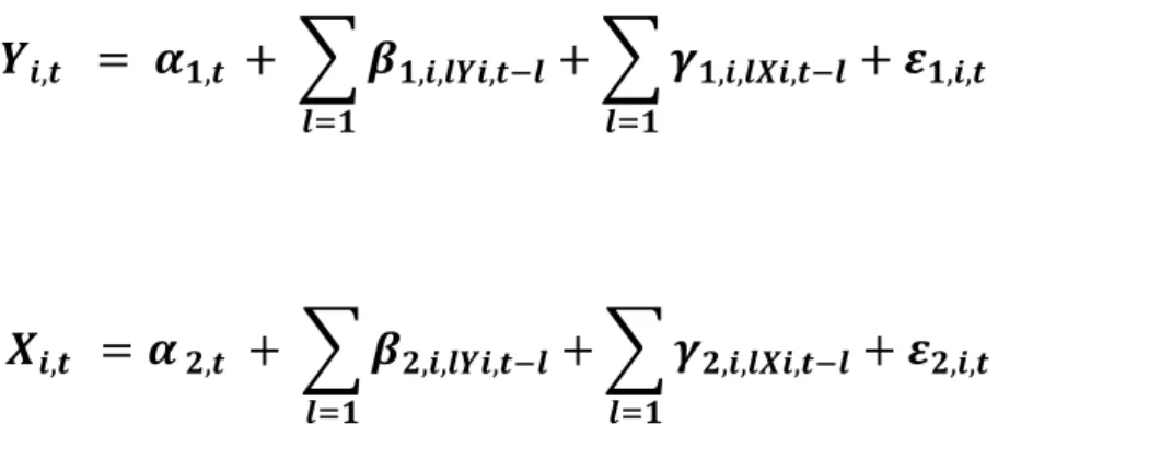
Bivariate Model

The possibility of Granger causality between GDP and EX can be investigated using the following finite-order vector autoregressive (VAR) models:

∑

∑

∑

∑

Where the index refers to the country ( = 1,2...N), equals the time period ( = 1,2...T), is the lag, represents white-noise term, and denote respectively, the Y=ΔLGDP and X=ΔLEX; and are difference stationary I(1) due to preliminary outcomes of the tests which show a

unit root at the level of the data. Accordingly, delta represents the first difference operator. With respect to this system of equations, country exhibits one way Granger causality from

to if in (1) not all are zero and in (2) not all are zero. The reversed relationship of

Granger causing is examined if in (1) all are zero and in (2) not all equal zero. There

is bidirectional Granger causality between and in case that in both equations (1) and (2)

neither all _{nor all} equal zero. Lastly, there is no causal relationship among the two

variables if all _and are zero. This definition implies one-period-ahead causality (Dufour and Renault, 1998).

In matrix notation, the VAR models of k variables for the ith _{panel member can be written as:}

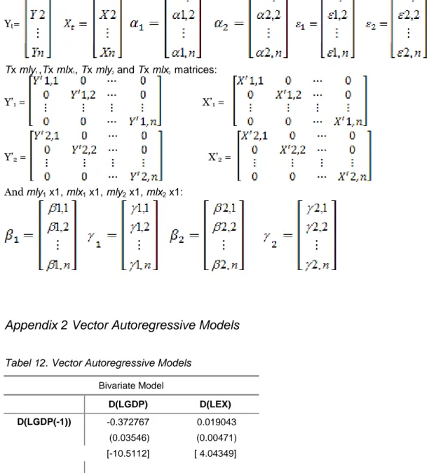
Where Yi and Xi are Tx1 vectors of the observed values of Y and X; Y’1,i, Y’2,i, X’1,i, X’2,i represent

T mly1 ,T mlx1, T mly2 and T mlx2 matrices of lagged values of Y and X, ε 1,i and ε2,i are T 1

vectors of values of the white-noise variables, α denotes the intercept terms and β and

are

in a decomposed matrix form is provided in Appendix 1.

Trivariate Model

For the second part of the empirical analysis, the logarithm of the variable of trade openness is included resulting into the following two generalized augmented variants of (1) and (2):

∑

∑

∑

∑

∑

∑

Where ₍ =1, 2, 3) denotes the lagged values of LOPEN and is mlz1 1 and mlx2 1

system, this variable is taken as an auxiliary variable and will not be involved in the Granger causality analysis.

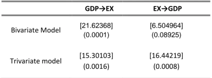
The final step of the empirical estimation is to test the whether 1,1= ... = 1, and 2,1

= … =

with individual Wald tests. Under the null hypothesis the parameter restrictions have a limiting

2 _{distribution with degrees of freedom corresponding to the maximum lag. If all 2i’s and 1i’s}

equal zero there is no Granger causality relationship.

3.3 Method

To test the nature of the association between the two variables and to avoid spurious regression, the empirical analysis follows these steps: The series are tested for stationarity by unit root tests. Motivated by the presence of a unit root in the time series, the long run cointegrating relationship between the variables is tested. In the final step the Granger causality relationship between the two variables is investigated by performing Wald tests within a finite order Vector Autoregressive (VAR) framework and on each individual cross section.

As concluded by Lee et al. (2004), in general all measures of trade openness are connected to the growth rate, therefore they might be simultaneously endogenous with economic growth. This increases the likelihood of an estimation bias stemming from simultaneous or reverse causation. Gujarati (1995) identified the VAR model as an exact simultaneous testing method because all variables are treated as endogenous considering the response in the system.

The rest of this chapter discusses in detail the estimation of the (1) and (2) bivariate systems, however all procedures apply to testing the variable of trade openness and to estimating the (5) and (6) trivariate equations.

3.3.1 Lag Length Selection

An important aspect of empirical research is the selection of the appropriate number of lags which need to be included in the empirical model. The lag length (k) has to be properly selected to ensure that the residuals empirically follow a white noise process. It has been observed that the power properties of the unit roots tests are sensitive to the number of lagged terms (k) used (Maddala et al. 1998). An extended lag structure may over specify the dynamics of the response, which will result in overstating the effects of past history while failing to impose relevant restrictions on the regression model. Lag structures may be restricted in order to reduce predictor dependencies, however, excluding predictors which are of significant value to the model may cause problems of under specifying the estimation dynamics. As a result, the effects of past history upon the model will be undervalued. Moreover, as referred by Maddala et al. (1998), specification of too few lags in the Johansen procedure causes specification distortions, and over specification of lags leads to loss of power. In such chances, it is more efficient to decide on a smaller lag (Maddala et al., 1998, pp. 334).

The adequate lag length can be determined using model selection criteria which provide results of the following test statistics: the sequential modified LR test statistic (LR), Final Predictor Error test (FPE), Akaike Information Criterion (AIC), Schwarz Bayesian Information Criterion (SBIC) and the Hannan-Quinn Information Criterion (HQC). As optimum lag selection criteria for this model is chosen the value which minimizes the Akaike (1974) and the Schwartz Information Criterion. As suggested by Ng and Perron (1995) both methods choose (k) proportionally to logT. As in most empirical research, the paper follows a sequential general-to-specific strategy selection. That is, starting with a maximum lag length k(max) and reduce the

number of lags until reaching significance. Results from the optimum lag length selection criterion often might support different lag lengths, however, in the case of the current model the

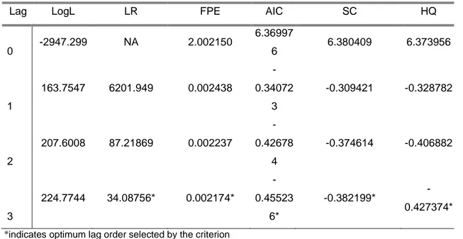
LR, FPE, AIC,SC and HQ tests show congruent test statistics results on the inclusion of 3 lags. The results of the test are presented in Table 2 below.

Table 2. VAR Lag Order Selection Criteria

Lag LogL LR FPE AIC SC HQ

0 -2947.299 NA 2.002150 6.36997 6 6.380409 6.373956 1 163.7547 6201.949 0.002438 -0.34072 3 -0.309421 -0.328782 2 207.6008 87.21869 0.002237 -0.42678 4 -0.374614 -0.406882 3 224.7744 34.08756* 0.002174* -0.45523 6* -0.382199* -0.427374*

*indicates optimum lag order selected by the criterion

3.3.2 Unit Root test

Before conducting an analysis it is first necessary to investigate whether the data set is stationary. This is tested using unit root tests. When specifying a unit root test, the decision of including appropriate deterministic components is vital since the resulting test statistic is dependant and influenced by them. A testing strategy is required in order to decide whether an intercept or an intercept with a trend should be included. Including too many of these deterministic regressors causes weaker results and increased probability of committing a Type 2 error. On the other hand including too few of them causes a bias in the test towards the null hypothesis and increases probability of committing a Type 1 error (Elder J. and Kennedy P. E., 2001). As proposed by Wolters and Hassler, (2006), a trend in the test regression should be included whenever a series is suspicious of a linear trend after a visual interpretation, since decision may not rely on the standard t-statistic of the estimated coefficient of the time regressor.

For this reason a basic type graph on the individual cross sections was composed and an upward stochastic trend in the variable of LEXP and LGDP was clearly observable. Real GDP has clearly grown between the years of 1971-2014. While the economies of the different countries have experienced periods of expansions and recessions, real GDP has been experiencing a gradual increasing trend. This is not a surprising fact as it is exhibited by several economic theories that technological advancement and increase in human capital endowments causes economic growth, both of which are present in the OECD circle. Furthermore, GDP is a variable which does not change dramatically from one period to the next, but rather follows a cyclicalpattern. For the graphs depicting the logarithm of exports, among the individual cross sections is also observable an overall upward trend. The long-term trend has been in the direction of expanding trade and increasing multinational integration, despite some unpredicted shocks which have periodically interrupted or reversed it (Jara, A., Low, P., 2013).

The size of the sample, in a large part, could determine which test is the most appropriate in certain cases. For a dataset with relatively small number of panels and an extensive time period, it is assumed that N is fixed or tends to infinity at a slower rate than T, (T → ∞, N finite or infinite). The meta analysis suggested by R. A. Fisher (1932), connects the p-values from

independent tests in order to obtain an overall test statistic and can be used for an unbalanced panel data set. Guided by the above mentioned factors, the model will be tested for a unit root Fisher type ADF test, allowing for a constant and a linear trend and employing a maximum of three lagged values. The unit root test is presented by the following equation:

=

where Δ

=

In the estimated equation if ρ , this indicates the presence of a unit root and confirms non stationarity. Next, by examining if the coefficients α and/or β are equal or differ from 0 we can see if there is a trend in the model.

The tested null and alternative hypotheses are determined as:

H

: ρ for all

H

: ρ< for at least one

Namely, the null hypothesis being tested is that all cross sections contain a unit root and the alternative is that at least one cross section is stationary. This test allows for stationarity in some of the cross sections, while others are non-stationary.

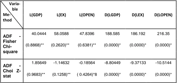
The test is performed on the level of the variables, it includes both intercept and a trend and it employs 3 lags. The results from the tests clearly show we cannot reject the null hypothesis at the 5 per cent level of significance, therefore all countries are not I(0). The conclusions are withdrawn from the results obtained in Table 3 and Table 4. Thus, it can be concluded that LGDP and LEX are difference stationary Yt I(1), Xt I(1).This implies that β=0, and a stochastic

trend with a drift is created by α≠0 (since yt is growing). Hence, there must be a positive or

negative α to generate a trending drift in yt. Therefore, the model is a random walk with a drift

process. Since the variables are integrated of order one, I(1), the level of the time series contains a unit root in its autoregressive part.

Table 3. Fisher-ADF Unit Root Test Varia-

ble Me-

thod

L(GDP) L(EX) L(OPEN) D(LGDP) D(LEX) D(LOPEN)

ADF - Fisher Chi-square 40.0444 58.0588 47.8396 188.585 186.192 216.35 (0.8868)** (0.2620)** (0.6381)** (0.0000)* (0.0000)* (0.0000)* ADF - Choi Z-stat 1.85649 -1.14632 -0.18564 -8.80449 -9.37133 -10.5144 (0.9683)** (0.1258)** ( 0.4264)*8 (0.0000)* (0.0000)* (0.0000)* ** Probabilities for Fisher tests are computed using an asymptotic Chi

-square distribution. All other tests assume asymptotic normality. H0: Presence of a unit root (individual unit root process)

Differencing is one of the methods which convert a nonstationary series of variables into stationary. Since Yt I(1), Xt I(1), the data needs to be differentiated d times before it becomes

stationary, then it is said to be integrated of order d, I(d). Taking the first-difference of a time series indicates the sequence of change from one period to the next. If Yt stands for the value of

the time series Y in period t, then the first difference will be equal to Yt-Yt-1, ( LGDPt - LGDPt-1

and LEXt - LEXt-1). As a result, both variables are stationary at Delta Yt I(0), Delta Xt I(0).

Hence, the empirical model will be estimated using LGDP and LEX instead of LGDP and LEX. The test reports the same results for the variable of LOPEN, therefore in the augmented systems (5) and (6) will be used t=D(LOPEN).

Table 4. Individual unit root tests Cross

Section LGDP LEX LOPEN D(LGDP) D(LEX) D(LOPEN)

AUS 0.5818 0.2348 0.2487 0.0016 0.0005 0.0002 AUT 0.6267 0.6820 0.7419 0.0424 0.0259 0.0125 BEL 0.1636 0.1598 0.3386 0.0098 0.0023 0.0027 DNK 0.4771 0.0988 0.5863 0.0024 0.0029 0.0023 FIN 0.8191 0.4307 0.4477 0.0357 0.1330 0.0996 FRA 0.6375 0.5102 0.5772 0.0018 0.0573 0.0408 DEU 0.8330 0.7218 0.7989 0.1369 0.0511 0.0299 GRC 0.8959 0.7604 0.4890 0.0067 0.0128 0.0098 ISL 0.8168 0.7764 0.9504 0.0779 0.0305 0.1600 IRL 0.3670 0.3271 0.3316 0.1332 0.1795 0.1814 ITA 0.4000 0.5234 0.7613 0.0014 0.0795 0.0476 JPN 0.2475 0.8488 0.9427 0.6574 0.0353 0.0100 KOR 0.2435 0.5519 0.7682 0.1133 0.0797 0.0846 LUX 0.4833 0.2429 0.5692 0.2183 0.0090 0.0436 MEX 0.5401 0.3289 0.1656 0.0635 0.0330 0.0064 NLD 0.8301 0.4852 0.7222 0.0840 0.0026 0.0032 NZL 0.6883 0.0256 0.1566 0.1045 0.0222 0.0047 PRT 0.5743 0.5749 0.2816 0.1226 0.0151 0.0019 ESP 0.0018 0.0167 0.2061 0.0009 0.1433 0.1300 SWE 0.3647 0.4058 0.3998 0.0003 0.1062 0.0262 CHE 0.9928 0.8302 0.0602 0.6376 0.0402 0.0019 TUR 0.8613 0.3030 0.4091 0.0887 0.1005 0.0661 USA 0.6559 0.3010 0.2425 0.0171 0.0418 0.0288 CAN 0.9866 0.7770 0.8490 0.0049 0.2536 0.2132 GBR 0.8358 0.1647 0.2203 0.0125 0.0320 0.0153 NOR 0.9770 0.3479 0.2305 0.5752 0.0134 0.0016 Note: The given values represent the probabilities

The results presented in Table 3 and Table 4 indicate that the level series and the error terms of the level series relationships are non-stationary. After differencing, we can reject the null hypothesis at the 1 percent level of significance, meaning that D(LGDP), D(LEX) and D(LOPEN) are stationary. The rejection of the null hypothesis in the Fisher-ADF test leads to the conclusion

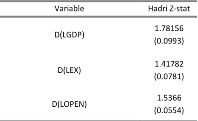
that at least one cross section is stationary, therefore to examine if the whole panel is stationary next is applied the Hadry (1999) test. Table 5 presents the results from the Hadry test statistic, from where it is observable that we cannot reject the null hypothesis, rather we accept it, meaning that all cross sections are difference stationary. This leads to the conclusion that, in each country and for the particular period under study, the processes are integrated and non-stationary which enables us to move to the main analysis (Johansen, 1988). Since both of the series are integrated of order one, the following step of the analysis will be to test for cointegration.

Table 5. Hadri test results

Variable Hadri Z-stat

D(LGDP) 1.78156 (0.0993) D(LEX) 1.41782 (0.0781) D(LOPEN) 1.5366 (0.0554)

Note: Probabilities of the test statistic are given in ( ) H0:Panel data does not contain a unit root

3.3.3 Cointegration test

The consecutive part of the analysis continues by applying all level series to test a Combined Johansen Cointegration test, in order to investigate if there is any long-run relationship between the two variables. The concept of cointegration confirms the existence of a long-run equilibrium where the economic system converges over time, or shows if they deviate significantly from one another (Abadir et al., 1999) . The Johansen Cointegration test is used to determine whether there exists a cointegration among a group of non-stationary series of variables (Dorsman et al., 2012). This test allows for more than one cointegration relationships and is more applicable in comparison to the Engle-Granger test. Johansen (1988) and Johansen and Juselius (1988) introduced a maximum likelihood estimation procedure which holds several advantages over the Engel Granger regression procedure. It assumes the cointegrating vector is unique and it considers the error structure of the underlying process (Dolado et al., 1990). The approach is based on the maximum likelihood estimation of the matrix (r-1), assuming normal distributed error terms. Maddala and Wu (1999) propose the Fisher test approach for testing cointegration in panel dataset by combining tests for individual cross sections in order to obtain a test statistic for the entire panel.

The test provides two test statistics for cointegration, the trace test and the maximum eigenvalue test. Respectively, the trace test’s null hypothesis tests if the cointegration rank equals r versus the alternative that the cointegration rank equals k. The null hypothesis for the maximum eigenvalue tests if the cointegration rank equals r against the alternative that the cointegration rank is r+1. The alternative hypothesis implies that Xt is trend stationary. Maddala

et al., (1998), suggest that the test statistic from the maximum eigenvalue may be more precise. Hence, guided by the above mentioned facts, in this analysis it is employed the Fisher Panel Combined Johansen Test. In order to perform this test it requires that all non-stationary time series contain the same number of unit roots (Lee 1997).This condition is fulfilled in the current dataset since Yt I(1), Xt I(1) and both of the variables become stationary when taking the first

difference, Yt I(0), Delta Xt I(0). The results from the cointegration test are displayed in

Table 6. Johansen Cointegration Test

Hypothesis of cointegration

Fisher Stat.*

(From Trace test) Prob.

Fisher Stat.* (From Max-Eigen test) Prob. None 67.10 0.0776 64.73 0.1106 At most 1 55.63 0.3396 55.63 0.3396

Probabilities () are computed using asymptotic Chi-square distribution Trend assumption: Linear deterministic trend

Lag: 3

In the absence of cointegration, we can conclude there is no long run relationship between Y and X, namely LGDP and LEX. The results are presented in Table 6 and Table 7 and show that the obtained probabilities from both tests are insignificant even at the 10% level of significance. Moreover, observing the individual cross section results presented in Table 7 it is clearly visible that there is strong evidence of no cointegration. This enables a conclusion that, in each country for each period under study, there is no cointegration relationship between the two variables. Therefore, we can reject both null hypotheses and confirm that these two variables have no long-run association, meaning that eventually they do not move together.

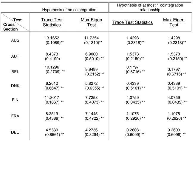
Table 7. Individual Cointegration test

Hypothesis of no cointegration

Hypothesis of at most 1 cointegration relationship Test Cross Section Trace Test Statistics Max-Eigen

Test Trace Test Statistics

Max-Eigen Test AUS 13.1652 (0.1089)** 11.7354 (0.1210)** 1.4298 (0.2318)** 1.4298 (0.2318)** AUT 8.4373 (0.4199) 6.9000 (0.5010) ** 1.5373 (0.2150)** 1.5373 (0.2150) ** BEL 10.1296 (0.2709) ** 9.9499 (0.2152) ** 0.1797 (0.6716) ** 0.1797 (0.6716) ** DNK 6.2612 (0.6647) ** 5.8272 (0.6355) ** 0.4339 (0.5101) ** 0.4339 (0.5101) ** FIN 11.8017 (0.1667) ** 7.7258 (0.4073) ** 4.0759 (0.0435) ** 4.0759 (0.0435) ** FRA 8.2519 (0.4389) ** 7.1445 (0.4722) ** 1.1075 (0.2926) ** 1.1075 (0.2926) ** DEU 4.5339 (0.8561) ** 4.2736 (0.8294) ** 0.2603 (0.6099) ** 0.2603 (0.6099) **

GRC 12.3533 (0.1408) ** 11.3922 (0.1356) ** 0.9610 (0.3269) ** 0.9610 (0.3269) ** ISL 3.3281 (0.9500) ** 2.2716 (0.9831) ** 1.0565 (0.3040) ** 1.0565 (0.3040) ** IRL 16.4097 (0.0363) ** 16.3051 (0.0235) ** 0.1046 (0.7463) ** 0.1046 (0.7463) ** ITA 6.3674 (0.6521) ** 5.3300 (0.6997) ** 1.0374 (0.3084) ** 1.0374 (0.3084) ** JPN 13.2246 (0.1068) ** 12.0123 (0.1102) ** 1.2123 (0.2709) ** 1.2123 (0.2709) ** KOR 7.7104 (0.4969) ** 7.5093 (0.4308) ** 0.2011 (0.6538) ** 0.2011 (0.6538) ** LUX 0.9703 (1.0000) ** 0.8572 (1.0000) ** 0.1132 (0.7365) ** 0.1132 (0.7365) ** MEX 6.3532 (0.6538) ** 6.2289 (0.5840) ** 0.1243 (0.7244) ** 0.1243 (0.7244) ** NLD 10.8345 (0.2219) ** 10.7900 (0.1650) ** 0.0446 (0.8328) ** 0.0446 (0.8382) ** NZL 12.6914 (0.1266) ** 11.7188 (0.1217) ** 0.9726 (0.3240) ** 0.9726 (0.3240) ** PRT 6.2945 (0.6607) ** 6.2795 (0.5776) ** 0.0149 (0.9025) ** 0.0149 (0.9025) ** ESP 13.7430 (0.0903) ** 12.7993 (0.0841) ** 0.9437 (0.3313)** 0.9437 (0.3313)** SWE 9.5262 (0.3189) ** 8.5878 (0.3221) ** 0.9384 (0.3327)** 0.9384 (0.3327)** CHE 12.8032 (0.1222) ** 8.9220 (0.2927) ** 3.8813 (0.0488)** 3.8813 (0.0488)** TUR 3.9984 (0.9037) ** 3.9676 (0.8627) ** 0.0308 (0.8606)** 0.0308 (0.8606)** USA 7.8199 (0.4848) ** 7.2130 (0.4642) ** 0.6069 (0.4360)** 0.6069 (0.4360)** CAN 10.6377 (0.2348) ** 7.0452 (0.4838) ** 3.5925 (0.0580) ** 3.5925 (0.0580)** GBR 9.6493 (0.3087) ** 7.9357 (0.3853) ** 1.7136 (0.1905) ** 1.7136 (0.1905) ** NOR 17.7061 (0.0229) ** 17.3175 (0.0160) ** 0.3886 (0.5330) ** 0.3886 (0.5330) ** **MacKinnon-Haug-Michelis (1999) p-values

Note: Probabilities are given in ()

According to this outcome, the empirical estimation of the model requires employing an unrestricted VAR and does not permit the usage of VECM. By that reasoning, the analysis proceeds by testing the short term dynamics of this relationship in a Granger causality test within a finite order unrestricted vector autoregressive (VAR) model.