Analysis of soil slopes utilizing acoustic emissions

ANALYSIS OF SOIL SLOPES UTILIZING ACOUSTIC EMISSIONS

*

e sE & a

All rights reserved INFORMATION TO ALL USERS

The qu ality of this repro d u ctio n is d e p e n d e n t upon the q u ality of the copy subm itted. In the unlikely e v e n t that the a u th o r did not send a c o m p le te m anuscript and there are missing pages, these will be note d . Also, if m aterial had to be rem oved,

a n o te will in d ica te the deletion.

uest

Published by ProQuest LLC (2018). C op yrig ht of the Dissertation is held by the Author.

All rights reserved.

This work is protected against unauthorized copying under Title 17, United States C o d e M icroform Edition © ProQuest LLC.

ProQuest LLC.

789 East Eisenhower Parkway P.O. Box 1346

An Engineering Report submitted to the Faculty and the Board of Trustees of the Colorado School of Mines in partial fulfil l m e n t of the requirements for the degree of Master of Engineering (Geological Engineer)

G o l d e n , Colorado Date £7/ Dr, A. K. Turner Thesis Advisor Golden, Colorado D r . Greg/Holden Department Head, Department of Geology

Abstract

Three active landslides located in Eagle County, Colorado were monitored with an acoustic emission (AE)

recording device for a eight month period beginning in January 1985, AE monitoring devices are used to detect the transient elastic waves generated by the release of energy within a material undergoing failure. The slides were also instrumented with piezometers and inclinometer boreholes. Groundwater data and displacement measurements gathered from these devices and data collected from surface movement observations were correlated with the AE data.

Significant increases in levels of AE activity were recorded at least 30 days prior to the observation of

movement at each of the slides. Rises in groundwater levels recorded at many of the observation stations appears to have triggered the failure of the slides. AE signals recorded after the initial failure of the slides were characterized by several cycles of increased activity followed by periods of r e l ative quiescence which correlated with periods of failure identified in surface movement observations.

This study has successfully demonstrated the

ability of a properly installed AE monitoring system to detect pre-failure stress increases in soil slopes. AE can be used as an early warning system for critical soil slopes,

road cuts, tailings dumps, dams, foundations and other civil structures. This new technology can be used to reduce

hazards to life and property in high risk areas.

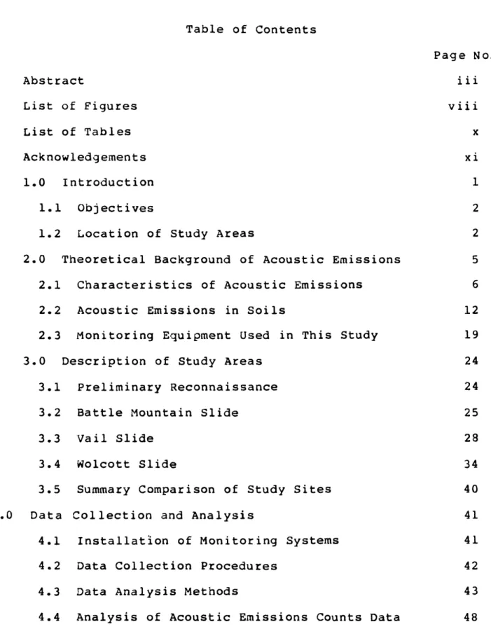
Table of Contents

Page No.

Abstract iii

List of Figures viii

List of Tables x

Acknowledgements xi

1.0 Introduction 1

1.1 Objectives 2

1.2 Location of Study Areas 2

2.0 Theoretical Background of Acoustic Emissions 5 2.1 Characteristics of Acoustic Emissions 6

2.2 Acoustic Emissions in Soils 12

2.3 Monitoring Equipment Used in This Study 19

3.0 Description of Study Areas 24

3.1 Preliminary Reconnaissance 24

3.2 Battle Mountain Slide 25

3.3 Vail Slide 28

3.4 Wolcott Slide 34

3.5 Summary Comparison of Study Sites 40 4.0 Data C o l l e c t i o n and Analysis 41 4.1 Installation of Monitoring Systems 41

4.2 Data Collection Procedures 42

4.3 Data Analysis Methods 43

4.4 Analysis of Acoustic Emissions Counts Data 48

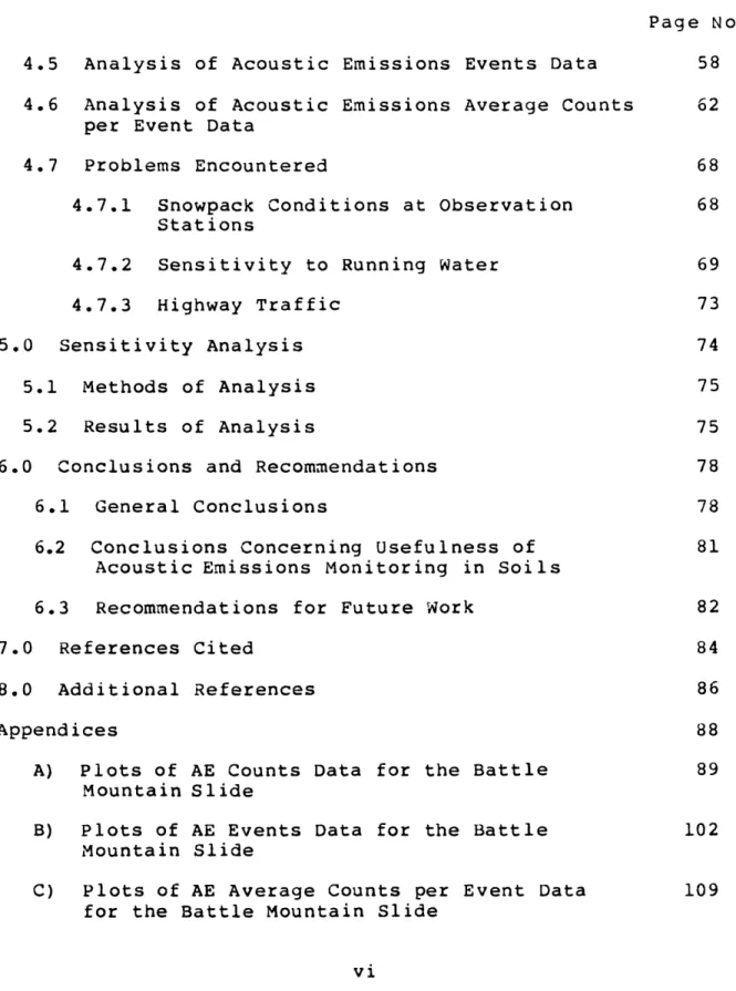
Table of Contents (con't)

Page No. 4.5 Analysis of Acoustic Emissions Events Data 58 4.6 Analysis of Acoustic Emissions Average Counts 62

per Event Data

4.7 Problems Encountered 68

4.7.1 Snowpack Conditions at Observation 68 Stations

4.7.2 Sensitivity to Running Water 69

4.7.3 Highway Traffic 73

5.0 Sensitivity Analysis 74

5.1 Methods of Analysis 75

5.2 Results of Analysis 75

6.0 Conclusions and Recommendations 78

6.1 General Conclusions 78

6.2 Conclusions Concerning Usefulness of 81 Acoustic Emissions Monitor ing in Soils

6.3 Recommendations for Future Work 82

7.0 References Cited 84

8.0 Additional References 86

Appendices 88

A) Plots of AE Counts Data for the Battle 89 Mountain Slide

B) Plots of AE Events Data for the Battle 102 Mountain Slide

C) Plots of AE Average Counts per Event Data 109 for the Battle Mountain Slide

Table of Contents (Con't)

Page No D) Plots of AE Counts and Groundwater Level Data 116

for the Battle Mountain Slide

E) Plots of AE Counts Data for the Vail Slide 123 F) Plots of AE Events Data for the Vail Slide 132 G) Plots of AE Average Counts per Event Data for 137

the Vail Slide

H) Plots of AE Counts and Groundwater Level Data 142 for the Vail Slide

I) Plots of AE Counts Data for the Wolcott Slide 145 J) Plots of AE Events Data for the Wolcott Slide 154 K) Plots of AE Average Counts per Event Data for 159

the Wolcott Slide

L) Plots of AE Counts and Groundwater Level Data 164 for the Wolcott Slide

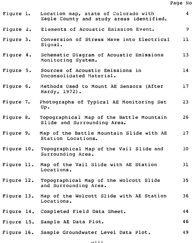
Figure 1. Figure 2. Figure 3. Figure 4. Figure 5. Figure 6. Figure 7. Figure 8. Figure 9. Figure 10. Figure 11. Figure 12. Figure 13. Figure 14. Figure 15. Figure 16. List of Figures Page No. Location map, state of Colorado with 4

Eagle County and study areas identified.

Elements of Acoustic Emission Event. 9 Conversion of Stress Wave into Electrical 11 S i g n a l .

Schematic Diagram of Acoustic Emissions 13 Monitoring System.

Sources of Acoustic Emissions in 14 Unconsolidated Material.

Methods Used to Mount AE Sensors (After 17 Hardy, 1972) •

Photographs of Typical AE Monitoring Set 23 Up.

Topographical Map of the Battle Mountain 26 Slide and Surrounding Area.

Map of the Battle Mountain Slide with AE 27 Station Locations.

Topographical Map of the Vail Slide and 30 Surrounding A r e a .

Map of the Vail Slide with AE Station 31 L o c a t i o n s ,

Topographical Map of the Wolcott Slide 35 and Surrounding A r e a .

Map of the Wolcott Slide with AE Station 36 L o c a t i o n s .

Completed Field Data Sheet. 44

Sample AE Data Plot. 46

Sample Groundwater Level Data P l o t . 49 viii

List of Figures (con't)

Page No Figure 17. Vertical Movement Recorded at the South 50

Flank of the Battle Mountain Slide

Figure 18. Plot of AE Counts Data at the Battle 51 Mountain Slide.

Figure 19. Plot of AE Counts Data at the Vail Slide. 53 Figure 20. Plot of AE Counts Data at the Wolcott 54

S l i d e .

Figure 21. Plot of AE Counts Data at the Vail Slide 57 at a Larger Scale.

Figure 22. Plot of AE Events Data at the Battle 59 Mountain Slide.

Figure 23 Plot of AE Events Data at the Vail Slide. 60 Figure 24. Plot of AE Events Data at the Wolcott 61

S l i d e •

Figure 25. Movement Recorded at the Wolcott Slide. 63 Figure 26. Plot of AE Average Counts/Event Data at 65

the Battle Mountain Slide.

Figure 27. Plot of AE Average Counts/Event Data at 66 the Vail Slide.

Figure 28. Plot of AE Average Counts/Event Data at 67 the Wolcott Slide.

Figure 29. Plot of AE Activity and Groundwater Level 72 Data at Statiôn CSM-2 of the Wolcott

Slide.

Table 1.

Table 2.

Table 3.

List of Tables

Pag e No, Materials Investigated Using Acoustic 7 Emissions M o n i t o r i n g .

Frequency Range of Monitoring Facilities 10 - Hertz (Hardy, 1972) .

Attenuation Rates of Soils Having Various 20 Moisture Contents (Lord, et al, 1977).

ACKNOWLEDGEMENTS

Sincere appreciation is extended to R.K. Barrett,

District III Geologist of the Colorado Division of Highways, for sponsoring this study. Funding from the Colorado

Division of Highways is acknowledged. Extra thanks are given to fell o w graduate students, Brendon Shine, Javier Fernandez, and Kahlil Nassar for their assistance in the field and for making their data a v a i l a b l e to me.

I t h a n k Dr. A.K. T u r n e r , c h a i r m a n , and Dr s. R.J. M i l l e r and K. Kolm, committee members, for their advisory

assistance and guidance in the preparation and presentation of this study.

A v e r y s p e c i a l t h a n k s is g i v e n to my wife, C h e r y l , and other members of my family for their unending support.

Finally, I would like to dedicate this report to Mr. F.W. Leighton of the U.S. Bureau of Mines. My interest in the field of acoustic emissions was the result of his

pioneering work in microseismics.

1.0 INTRODUCTION

This report presents the results of an anaylsis of the effectiveness of acoustic emissions monitoring as a method of determining the stability of soil slopes and as a means of predicting movement prior to failure. This study is part of a Colorado Division of Highways effort to characterize

landslides that are affecting major highways in Eagle C o u n t y .

The ability to determine the state of stress and

s t a b i l i t y of a soil m a s s has been a p r i m a r y o b j e c t i v e of the engineering community for many years. Present state-of-the- art instrumentation, such as inclinometers and t i 1 tmeters, yield v a l u a b l e information about the direction and amount of movement in a failing earth slope. However, they are only capable of measuring movements once failure has begun. The measurement of these displacements is excellent for

d e v e l o p i n g a model of the failure type. These methods do not, however, give any indication of the stress state of the soil mass or, more importantly, a warning of future

m o v e m e n t .

Soil pressure c e l l s are also used to monitor the

stability of earth structures. These instruments yield data on stresses in soil masses. However, they are r e l a t i v e l y

expensive and must be buried permanently in the soil mass. Furthermore, in order to collect soil pressure data,

electric wires or small diameter pneumatic tubing must extend to the surface. In the case of landslides, these w i r e s or t u b e s m a y be s e v e r e d once the s l o p e b e g i n s to fail.

There exists a need for the testing and evaluation of new and inexpensive instrumentation technologies that can provide an indication of the relative instability of a soil structure prior to failure.

1.1 Objectives

Specific objectives of this study include:

(1) The characterization of acoustic emissions (AE) in a ctive landslides;

(2) The determination of the effectiveness of AE monitoring in identifying pre-failure changes in

stresses in landslides; and

(3) The eva l u a t i o n of the effects of weather conditions and highway traffic on AE monitoring systems.

1.2 Location of Study Areas

landslides and data on AE activity were collected for an eight month period beginning in January and ending in August of 1985. The landslides studied include:

(1) The Battle Mountain Slide located on U.S. Highway 24 two m iles south of Minturn;

(2) the Vail Slide located on Interstate 70 in East Vail; and

(3) the Wolcott Slide located on Interstate 70 one mile east of W olcott (Fig. 1).

These slides experienced movement in previous years which resulted in extensive roadway repair operations.

Several other types of instrumentation, including piezometers and inclinometers, along with traditional

surveying methods, were also employed at each landslide. AE activity data were correlated with data c o llected from these other monitoring systems in order to eva l u a t e the results of the various types of instrumentation.

C

O

L

O

R

A

D

O

s

FI

GU

RE

1

Lo

ca

ti

on

Ma

p,

St

at

e

of

Co

lo

ra

do

wi

th

Ea

gl

e

Co

un

ty

an

d

St

ud

y

Ar

ea

s

I

d

e

n

t

i

f

i

e

d

2.0 THEORETICAL BACKGROUND OF ACOUSTIC EMISSIONS

Acoustic Emissions, commonly referred to AE, have also been c a l l e d microseismics, microsonics and subaudible rock noise (SARN). These techniques are designed to record "... the transient elastic waves generated by the rapid release of energy within a material " (Leaird and Plehn, 1984). While AE monitoring is a r e l a t i v e l y new technology, audible n o i s e has b een u s e d as a m e a n s of e v a l u a t i n g the state of stress of structures for hundreds of years.

Miners estimate the stability of underground openings by the a m o u n t of n o i s e e m i t t e d from s u p p o r t timbers. The conditions of rock p i l l a r s in mines are s i milarly evaluated u s i n g n o i s e as m e a s u r e of s t a b i l i t y . One of the first discoveries of subaudible noise was made in the late 1930's by U. S. B u r e a u of M i n e s w o r k e r s a t t e m p t i n g to m e a s u r e s e i s m i c v e l o c i t i e s in s t r e s s e d rock p i l l a r s (Obert and Duvall, 1942).

Obert and D u v a l l were attempting to ev a l u a t e the

stability of underground openings by measuring the seismic v e l ocity of rock p i l l a r s under various states of stress. Their experiments consisted of inducing a seismic wave and

recording the time required for the wave to travel from one side of a pill a r to the other. They found that their

recording system was prematurely triggered by unrelated

bursts of seismic energy. They postulated that these bursts of seismic energy were related pillar loading. Subsequent experiments confirmed that the quantity and duration of these bursts was a function of the state of stress of the p i l l a r s (Obert and Duvall, 1942).

AE monitoring has since been used by researchers to investigate failure in other media such as metals, concrete and composite m a t e r i a l s (Table 1) (Harris, et al, 1972: Liptai, et al ,1972). M u l t i channel AE monitoring has also proven to be very successful in detecting and locating leaks in pressurized v essels and pipelines. Recently, researchers at various universities and government research agencies h a v e been investigating the possibility of adapting this technique to the e v a l u a t i o n of soils (Koerner, et al, 1980).

2.1 Characteristics of Acoustic Emissions

Acoustic emissions, as with all seismic signals, occur as waveforms of varying frequency and amplitude. Acoustic emissions are characterized by transient displacements on the order of 0.00000001 inches and a period on the order of 10 to 1,000,000 cycles per second (Leaird and Plehn, 1984). A record of acoustic emissions g e n e r a l l y consists of

TABLE 1 Materials Investigated Using Acoustic Emissions Mom*torir

Material

Investigation

Soil

Rock

Civil Structures

Other

Dams, Emabankments

Cuts, Fills

Settlements

Lateral Movement

Laboratory

Mine Safety

Subsidence

Open Cuts

Concrete

Steel

Avalanche Control

Composite Materials

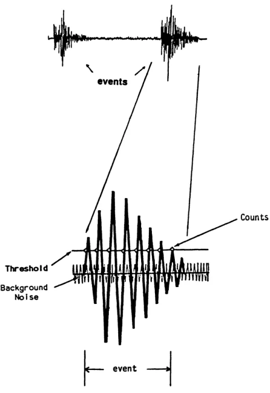
individual bursts or pulses separated by periods of relative quiescence (Fig, 2). AE monitoring systems count and

record the number of seismic events per sample interval which equal or exceed some preset threshold level of signal amplitude.

The threshold, or baseline, level is used to

distinguish between the background noise of the recording system and bursts of acoustic activity. Each time the AE signal exceeds this threshold value a count is recorded

(Fig. 2). Because the AE signal is a waveform, several counts are commonly identified within each pulse or event.

Investigators found that AE signals are emitted over a wide range of frequencies and that the range of frequencies u s e d in a s t u d y is a f u n c t i o n of the type of m a t e r i a l u n d e r

investigation (Hardy, 1972). Table 2 shows how AE

frequencies compare with other types of ground vibration studies and how the characteristic AE frequencies vary with types of m a t e r i a l .

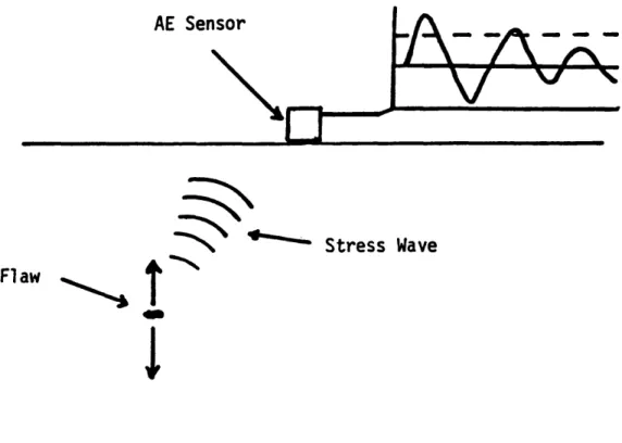
Acoustic emissions are detected by a highly sensitive accelerometer capable of measuring very minute vibrations in materials. The accelerometer converts the mechanical stress wave into a electrical signal (Fig. 3). A typical AE

monitoring system consists of, in addition to an

TYPICAL ACOUSTIC EMISSION RECORD

events

event

Counts

CM rs. 01

a

1

s

I

P i

ill

1

Iasi

i t S S S

T

^ E § i

ii

+

1

=

AE Sensor

Flaw

î

I

Stress Wave

and a recording device (Fig, 4).

2.2 Acoustic Emissions in Soils

Koerner, Lord and others at Drexel University, Philadelphia, Pennsylvania conducted several laboratory

experiments using soil samples and were able to identify two mechanisms of AE signal generation in stressed soils

(Koerner, et al, 1978).

Friction is the first, and probably most significant, mechanism for the release of acoustic energy in soils (Fig. 5). A failing soil mass undergoes several types of

deformation and at least one failure surface is developed. As the soil mass fails, individual particles of material in the failure zone(s) abrade one another. This abrasion

r e l e a s e s a g r e a t d e a l of e n e r g y in the form of heat and acoustic emissions. Abrasion activity in failure zones accounts for the greatest portion of microseismic energy in a failing soil mass.

Particle deformation is the second method by which acoustic emissions are generated (Fig. 5). This effect, while certainly present in soil masses, is best illustrated in a more brittle medium, such as rock. Studies conducted in underground coal mines have yielded a great deal of data

u « en u o c « en

FI

GU

RE

4

Sc

he

ma

ti

c

Di

ag

ra

m

of

Ac

ou

st

ic

Em

is

si

on

s

Mo

ni

to

ri

ng

Sy

s

t

em

FIGURE 5

Sliding Friction Rolling Friction

✓ V /

Degradation Dilation

Sources of Acoustic Emissions in Unconsolidated Material

on particle deformation (Obert and Duvall, 1942). When a p i llar of coal in an underground coal mine is subjected to

loads, the c o a l r e s p o n d s in s e v e r a l w a y s , one of w h i c h is coal hardening. As a pillar compresses in response to the changing stresses, the particles within the coal are

deformed and take on new characteristics. These responses result in the emission of acoustic signals. Even though particle deformation in soil masses is not a major

contributor to AE activity, it is present and must be considered •

Perhaps the most important finding of Koerner and Lord was that acoustic emissions are rapidly attenuated in

u nconsolidated materials (Koerner, et al, 1980). By

introducing a signal of known intensity into soil samples, they were able to determine that a significant portion of AE signals are lost in r e l a t i v e l y short distances.

The h i g h f r e q u e n c y AE s i g n a l s are a t t e n u a t e d m o r e r a p i d l y than the low f r e q u e n c y portion. A c c o r d i n g l y , the range of AE signals that can be detected is greatly reduced as the d i s t a n c e b e t w e e n the s o u r c e of AE s i g n a l s and the s e n s i n g d e v i c e increases. The m ost u s e f u l p o r t i o n of AE signals in soils is found in the higher frequencies (Table 2) and t h e r e f o r e the signa 1 - s e n s i n g i n s t r u m e n t s must be positioned close to the source of the AE activity. Because

f a i l u r e s in s o i l s are o f t e n d e e p - s e a t e d , p o s i t i o n i n g the accelerometer close to the source of the AE activity becomes d i f f i c u l t .

Koerner and his associates addressed this problem and tested several different methods of transmitting AE signals to a sensing accelerometer. Several types of signal

transmitters, commonly referred to as waveguides, were e v a l u a t e d (Koerner, et al, 1978). S t e e l , due to its high modulus of elasticity, was found to be the best signal c o n d u c t o r •

Several methods of mounting AE sensors, in addition to steel waveguides, have been used with varying degrees of

success (Fig. 6). Preexisting wellhead facilities hav e been used in studies at gas storage facilities. However, caution must be exercised when using well casing as a waveguide to

insure that the sensing device is not detecting AE activity related to fluid flow within the well. Borehole probes have also met with success but are also expensive. Burial of sensors has also been attempted but is limited to s h a l l o w failures or low frequency monitoring.

The California Department of Transportation investigated the possibility of using low frequency transducers placed in s h a l l o w boreholes (10 to 15 feet deep) and coupled with the soil by either filling the

FIGURE 6 1/2" steel pipe 2-200' A) Waveguide Mounting

" V m

s »

rv

1

r

E) Well bore Probe

Methods Used to Mount AE Sensors (S=Sensor, PA= Preamplifier, JB=Junction Box)(After Hardy, 1972)

borenole with water or by placing the transducer on the bottom of the hol e as shown in Figure 6 (McCauley, 1977). Because only the low frequency range of the AE activity was monitored (representing a small portion of the AE activity) a set of headphones was used by the operator to detect and count AE events.

This method of observation is presently being used by the California Department of Transportation to evaluate the stability of soil slopes which have already failed

(McCauley, 1977). This monitoring a l l o w s the operator to distinguish between various extraneous sources of noise and AE activity related to the stability of the soil slope. However, this system is limited in applications because it is not capable of detecting the higher frequency portions of AE signals that provide better resolution of AE activity and h e n c e a b e t t e r i n d i c a t i o n of the st a t e of s t r e s s of a soil m a s s .

The monitoring system employed for this Colorado Division of Highways (CDoH) investigation utilized one- half inch diameter steel piezometer tubes as waveguides but did not include headphones. The use of headphones would have greatly simplified the analysis of the records of AE activity at several of the sites. However, it would have been very difficult to count individual events emitted from

the failure surface and transmitted to the surface via the steel waveguides.

Koerner and Lord were able to quantify attenuation rates for different types of soils having various moisture contents (Koerner et al, 1980). The results of their

laboratory tests indicate that AE signal attenuation is a function of both grain size and moisture content. They f ound than a s i l t y sand at zero p e r c e n t water c o n t e n t had a lower attenuation rate than a clayey silt at the same water content (Table 3).

The moisture content of an unconsolidated material also g reatly affected the attenuation rate of AE signals. The results of laboratory tests conducted on silty sand samples of various moisture contents indicate that the presence of air in the soil voids can increase the attenuation values significantly. For example, changing the water content from zero to 12 percent lowered the attenuation by approximately 200 percent (Koerner, et al, 1980).

2.3 Monitoring Equipment Used in This Study

The AE monitoring system used for this project

consisted of the following components: (1) an accelerometer with a 30 kiloHertz resonance frequency; (2) a 15 to 45

TABLE 3 Attenuation Rates of Soils Having Various Moisture Contents

(Lord, et. a l ., 1972)

Material

Moisture Content

Attenuation Rate

_ _ _ _ _ _

(weight %)

(dB/foot)

Silty Sand

0

40

Clayey Silt

0

57

6

41

kiloHertz bandpass filter; (3) a signal conditioning unit; and (4) a signal analyzing unit. The last two pieces of equipment were contained in a single instrument. The signal conditioning/analyzer device was a single channel unit. M odel 204G, manufactured by Acoustic Emissions Technology Corporation (AET). This AET device was fully self-

contained, designed for field use, and required no modifications. It was equipped with variable gain and sampling rates, an adjustable threshold setting, and a

digital display screen. It is designed to record both the n u m b e r of c o u n t s and the n u m b e r of e v e n t s for a g i v e n s a m p l e period. This period can be selected up to a maximum of one minute, or altern a t e l y a "continuous" recording mode may be selected. An AET model AC30L accelerometer was used for this study.

In order to attach the accelerometer to the waveguide (made of one-half inch steel pipe, as described previously), a three-inch diameter steel platen was fitted with a set of pipe threads that matched those of the one-half inch pipe. This platen was constructed so that it could be easily removed from the waveguide to a l l o w access for groundwater m e a s u r i n g .

A shield designed to prevent wind-borne acoustic signals from reaching the accelerometer was used. It

consisted of a f i v e - g a l l o n plastic container lined with 2- inch foam. The container was inverted and placed over the platen and accelerometer and secured by weights to prevent noise generated by movement of the shield. Photographs of a typical AE monitoring set up are given in Figure 7.

F I G U R E 7 P h o t o g r a p h s of T y p i c a l A E M o n i t o r i n g Se t U p

ARTHUR LAKES LIBRARY COLORADO SCHOOL of MINES

3.0 DESCRIPTION OF STUDY AREAS

3.1 Preliminary Reconnaissance

Prior to the installation of monitoring equipment, a reconnaissance trip was made to each of the study areas. Mr. Robert K. Barrett, District III geologist with the Colorado Division of Highways, in whose district the study areas are located, was present and related the history of oach landslide. After inspecting each site, a set of

combined acoustic emission monitoring/groundwater piezometer stations was proposed. These stations were to be located near the crown, m i d d l e and toe areas of the Battle Mountain and Vail landslides and in the upper portion of the Wolcott Slide. An additional monitoring location was chosen

outside the boundaries of each slide so that background AE activity recordings could be made during the course of the study for comparison with the landslide AE activity

readings. Finally, locations for at least one inclinometer hole per landslide were identified. Installation of these monitoring stations was accomplished in the winter of

3.2 Battle Mountain Slide

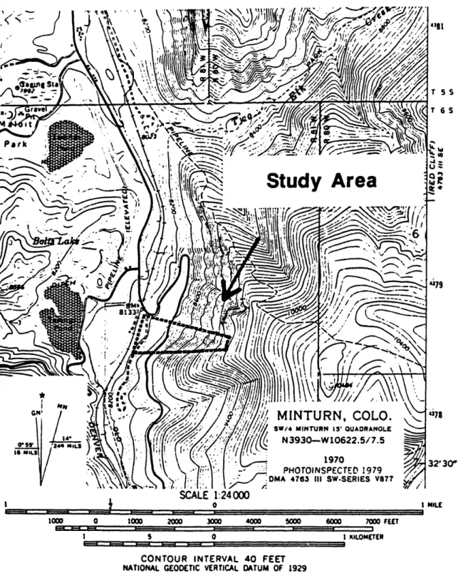
The Battle Mountain landslide is located in Section 1 of Township 6 South, Range 81 West (Sec 1, T 6S, R81W) on U.S. H i g h w a y 24 , two m i l e s s o u t h of M i n t u r n (Fig. 8).

This site, situated on the west flank of Battle Mountain, is a deep-seated rotational failure. It has been subjected to severe recurrent movement for several years that has made n e c e s s a r y the r e p e a t e d repa i r of U.S. H i g h w a y 24. In p r e v i o u s y e a r s this s l i d e has been s t a b l e t h r o u g h o u t the w i n t e r m o n t h s and b e c a m e a c t i v e in the s p r i n g and summer months. It was k n o w n that the l e v e l of g r o u n d w a t e r in the

landslide fluctuated with the seasons, with highs recorded in the s p r i n g and s u m m e r and the l ows o c c u r r i n g in the f a l l and winter months (Barrett, personal communication).

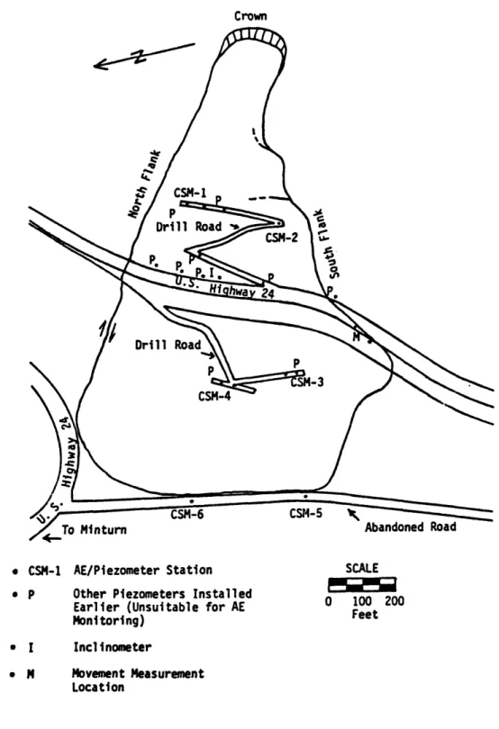
A total of six combination AE/Groundwater piezometer stations were installed at the Battle Mountain study area (Fig. 9). Two stations, CSM-1 and CSM-2, were located in the upper portion of the landslide. Station CSM-1 was l o c a t e d in the u p p e r p o r t i o n of the s l i d e and d r i l l e d to a total depth of 58 feet. Station CSM-2 was located

approximately 20 feet from the right scarp and had a total depth of 20 feet. These two stations were completed in red, micaceous, sandy, clayey silt.

% a a BUi | W.

Study Area

i

MINTURN, COLO.

DMA 4763 III SW-SERIES V877

Çÿ .

32'30"

SCALE 1:24000

o i m il e

1000 1000 2000 3000 4000 5000 6000 7000 FEET

I KILOMETER CONTOUR INTERVAL 40 FEET

NATIONAL GEODETIC VERTICAL DATUM OF 1929

FIGURE 8 Topographical Map of the Battle Mountain Slide and Surrounding Area

Crown CSM-1 Drill Road >, CSM-2 IV. Drill Road ;SM-3 CSM-4 CSM Abandoned Road To Minturn • CSM-1 AE/Piezometer Station • P Other Piezometers Installed

Earlier (Unsuitable for AE Monitoring) • I Inclinometer • M Movement Measurement Location SCALE 0 100 200 Feet

FIGURE 9 Map of the Battle Mountain Slide with AE Station

Locations

Observation stations CSM-3 and CSM-4 were located in the central portion of the slide. Station CSM-3 was 42 feet d e e p and s t a t i o n C S M - 4 was d r i l l e d to a d e p t h of 155 feet. Both CSM-3 and CSM-4 were located red micaceous, sandy, clayey slit interbedded with clasts of fine to medium grained arkosic sandstone and variegated shales.

Stations CSM-5 and C S M -6 were installed near the toe of the l a n d s l i d e on an a b a n d o n e d h i g h w a y to d e p t h s of 53 and 150 feet, respectively. Station C S M -6 was completed in the same materials as CSM-3 and CSM-4. Station CSM-5, located very close to a bedrock outcrop, penetrated a thin layer of the p r e v i o u s l y described soils before reaching a fine­

grained quartzose sandstone.

Prior to this study, several groundwater piezometers and an inclinometer test hole had been installed on the Ba ttle Mountain slide. These installations, while useful for water level and movement observations, were completed w i t h P V C c a s i n g and w e r e not c o m p a t i b l e w i t h the AE

monitoring system since they could not be used as waveguides.

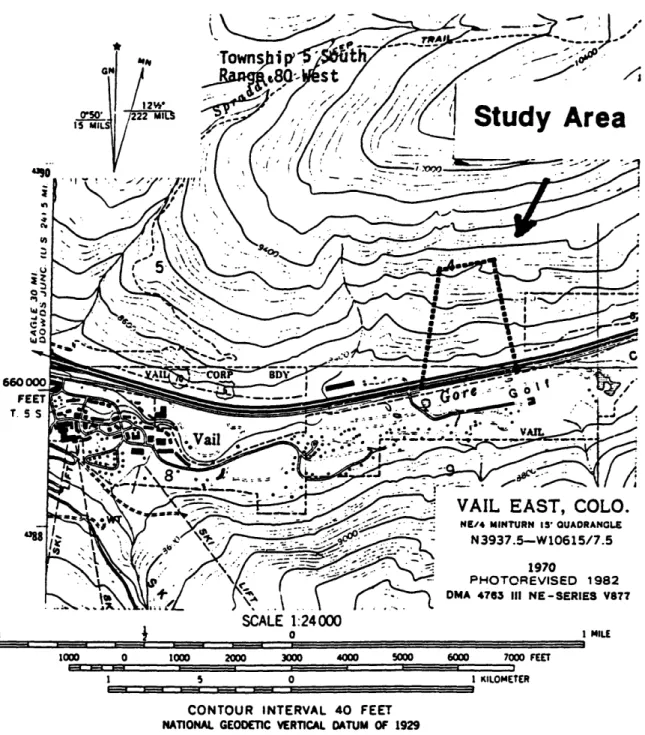
3.3 Vail Slide

side of the west-bound lanes of Interstate 70 in East Vail (Fig. 10). This was the site of significant movement in May, 1984. The CDoH wanted to determine the stability of the slope and, if it is not stable, to identify appropriate

remedial actions.

The Vail landslide was monitored with a total of five combination AE/Groundwater piezometer stations and one

inclinometer hole (Fig. 11). Two of the AE stations, CSM-1 and C S M - 2 , w e r e l o c a t e d as far up the s l i d e as p o s s i b l e w i t h the d r i l l i n g equipment. The slide is on Forest Service land and a temporary drill road was constructed, but this was regraded and mulched by early May, according to the terms of the Forest Service permit. Stations CSM-3 and CSM-4 were positioned lower in the slide along the temporary road and s t a t i o n C S M - 5 was l o c a t e d near the toe of the s l i d e on the north shoulder of the west-bound lanes of Interstate 70. The inclinometer hole was d r i l l e d near station CSM-4 in the middle portion of the landslide. All of these stations were completed in a red micaceous silt containing occasional

clasts of feldspathic sandstone.

Unexpected, and seemingly inconsistent, measurements of groundwater l e v e l s and displacement were recorded at several locations within the slide. Groundwater l e v e l s recorded at each piezometer station identified a rise in the

Township’

VAIL EAST, COLO

M E /4 MINTURN IS’ QUADRANGLE N3937.5—W 10615/7.5 1970 P H O T O R E V IS E D 1 9 8 2 DMA 4763 III N E -S E R IE S V877 V \ \ SCALE 1:24000 1000 0 1000 2000 3000 4000 5000 6000 7000 FEET 1 5 0 1 KILOMETER

CONTOUR INTERVAL 40 FEET NATIONAL GEODETIC VERTICAL DATUM OF 1929

FIGURE 10 Topographical M a p of the V a i l Slide and Surrounding Area

/

CSM-1

CSM-2

EDM-6

CSM-3

_{Slump Cracks}

EDM-3

EDM-4

CSM-4 I

EDM-1

Road Cut

CSM-5

1-70 west

1-70 east

• CSM-1 AE/Piezometer

• I

Inclinometer

SCALE

EDM-6 Movement Measurement

Location

0

100

200

Feet

p o t e n t iometrie surface in the spring. This rise in

groundwater l e v e l s appears to be responsible for the renewed movement of the slide. However, the increase was of short duration and was followed by a decline to a level several tens of feet below the identified slip surface. A decline recorded near the crown is not unusual, but the decline observed at the toe of the slide was inconsistent with the continued movement of the slide.

Upon plotting the groundwater level data on cross sections, it was observed that the extremely low

p o t e n t iometric surface coincided with a basal gravel unit which was also mapped in the v a l l e y b e l o w the slide

(Fernandez, 1986). It now seems likely that the slotted observation w e l l s acted as drains and a l l o w e d the n o r mally saturated soil to l o c a l l y drain to the more permeable

underlying gravels.

Groundwater l e v e l s recorded in the inclinometer

borehole did not f o l l o w the same pattern, but remained at a very high level for most of the study period. These

anomalously high groundwater l e v e l s were possibly an

artifact of the techniques used to install the inclinometer station. It is now b e l i e v e d probable that water trapped in the impermeable inclinometer casing during construction drained at a much slower rate than normal and resulted in

the high water level readings.

The inclinometer was not completed until after the

slope began to fail. The PVC casing was immediately sheared off. This prevented the inclinometer tool from reaching the stable base of the hole. This is critical because

displacement c alculations are based on the assumption that the bottom of the hole is not moving. Because the necessary baseline measurements could not be collected to the bottom of the hole, CDoH personnel therefore elected not to collect additional inclinometer data at this location. Measurements of surficial slide movement were conducted using a variety of traditional surveying techniques. Also six EDM

(electronic distance measuring) stations were installed on the s l i d e and read m o n t h l y f rom M a y to August.

The results of these measurement activities also proved difficult to interpret. The slide appears to have two

divergent directions of movement. While the dominant mo vements are downs lope to the south, the western half of the slide moves sl i g h t l y to the west while the eastern half of the s l i d e m o v e s s l i g h t l y to the east. W h i l e the dat a are

incomplete, features identified in both h a l v e s of tne slide indicate that the western portion is failing in a fairly deep rotational fashion and the eastern half, located

a series of wedges of soil (slumps) due to an oversteepening of the slope during highway construction. The degree to which the rotational and slump failures are related is unknown. Regardless of the situation, records of AE

activity appear to track only the rotational failure in the western portion of the slide and the discussion of the

r e s u l t s of the a n a l y s i s of the AE dat a w i l l be l i m i t e d to this portion of the study area.

3.4 Wolcott Slide

The Wolcott slide is located along the Interstate 70 right-of-way in Sections 23 and 26 of T4S, R83W; 1.5 miles east of the Wolcott exit (Fig. 12). This slide is traceable across bor.h the east- and west-bound lanes of Interstate 70 as well as the frontage road (U.S. Highway 6). This site has been subjected to recurrent movement every spring for the past several years. These movements have severely damaged all of the roadways and have made costly repairs necessary. The CDoH would like to stabilize this slide in order to minimize future repairs.

Six AE monitoring stations and three inclinometer holes were installed at the Wolcott slide (Fig. 13). Three of the AE stations, CSM-1, CSM-2 and C S M - 6 , were

Study Area

5

CONTOUR INTERVAL 40 FEET DASHED LINES REPRESENT 20-F00T CONTOURS NATIONAL GEODETIC VERTICAL DATUM OF 1929

Crown U.S Highway 6 Irrigation Canal • CSM-1 AE/Piezometer Inclinometer Movement Measurement Location SCALE Feet

FIGURE 13 Map of the Wolcott Slide with AE Station Locations

p l a c e d in what was t h o u g h t to be the u p p e r p o r t i o n of the slide. Plane-table mapping of the study area subsequently revealed that two of the stations, CSM-2 and C S M - 6 , were a c t u a l l y installed outside of the slide. Two stations, CSM- 7 and C S M -9, w e r e l o c a t e d in the c e n t r a l part of the

landslide. Station CSM-7 was installed on the south

shoulder of the east-bound lanes of Interstate 70, and CSM-9 was located in the median between the east- and west-bound

lanes of Interstate 70. Two inclinometer holes were d r i l l e d on the south shoulder of the east-bound portion of

Interstate 70 and the third inclinometer hole was positioned in the median between the west-bound portion of Interstate 70 and the frontage road. Two benchmark locations were also installed outside of the landslide for survey control

points. One of these benchmarks, constructed with one-half inch steel pipe, was used to record background l e v e l s of AE activity for the study area. All of the holes d r i l l e d at the Wolcott Slide penetrated a thin mantle of soil underlain by a gray sandy silt, a mas s i v e quartzose sandstone and

thinly bedded gray silty shales.

Drilling and coring activities conducted during the installation phase identified a r e l a t i v e l y s h a l l o w dip-slip failure located in bedrock. The failing mass of soil and rock was approximately 25 feet thick. The underlying

failure zone was located in a zone of thinly bedded sandstones, si 1 tstones and shales. The inclinometer identified at least two major slip surfaces and the data suggest that others may be present.

The s l i d e is s i t u a t e d nea r the axis of a v e r y l a r g e east-west trending syncline in the Cretaceous Dakota

sandstones, si 1 tstones and shales. The dip of the bedrock in this area is a p p p r oximate1 y 30 degrees to the north and the resultant topography is a uniformly dipping hillslope. The hummocky texture of the study area and surrounding slopes indicates that the W olcott Slide is one of many

failures that have occurred along slip surfaces found within the thinly-bedded shales.

It appears that changing groundwater conditions were a key factor in the reactivation of movement at this site. Field observations suggest several ways in which water has affected the stability of this area (Nassar, 1986). First, movement of the slide was probably triggered by rising

groundwater l e v e l s during the spring runoff. Second, the effect of the high groundwater l e v e l s was intensified by the

lack of proper surface runoff management along the

Interstate right-of-way. Surface runoff was allowed to pond along the south shoulder of the east-bound lanes and in the median between the east- and west-bound lanes of Interstate

70 and U.S. Highway 6. Third, the irrigation canal located along the toe of the slide immediately be l o w U.S. Highway 6 has been disturbed by the movement of the slide. During the spring runoff period, water overflowed the canal banks and began to pond on the slide. Such saturation no doubt

reduces the stability of the slide.

It is uncertain whether the canal, through normal leakage, caused the slide to become unstable which consequently disturbed the canal, or whether the slide became unstable due to spring runoff derived groundwater resulting in the disturbance of the canal. Regardless of the order of events, seepage from the canal is presently adding to the instability of the study area.

One natural cause of the instability is the erosive a c t i o n of the E a g l e R i v e r w h i c h has a m e a n d e r b e n d at this point. The erosive energy of the river on the outside of the meander removes material from the toe continuously, with periods of maximum erosion occurring during the high runoff season. P l a n e - t a b l e m a p p i n g at the toe of the s l i d e

identified a series of wedge-shaped slices of soil moving into the river. The measured vertical displacement of some of these slices was as great as four feet.

3.5 Summary Comparison of Study Sites

The three study sites represent a variety of slope and hydrological conditions. The Battle Mountain Slide and the Vail Slide are deep-seated rotational failures of soil and colluvium. The Wolcott Slide is a s h a l l o w dip-slope failure that is failing along a bedding plane in bedrock. Although movement of all three slides appears to be

triggered by rising groundwater associated with spring runoff, the structural setting of each of the slides is significantly different.

The Battle Mountain and the Vail slides are located on larger ancient landslides which were reactivated. At the V a i l S l i d e , this was c a u s e d w h e n a cut s l o p e was m a d e at the toe during construction of Interstate 70. At the Battle Mountain Slide, the cause of reactivation is more complex and it may never have been truely stable since the original

failure. The Wolcott Slide was probably activated by the continuous removal of material at the toe by the erosive action of the Eagle River.

These slides provide an excellent opportunity to characterize AE activity in a variety of geological conditions.

4.0 DATA COLLECTION AND ANALYSIS

4.1 Installation of Monitoring Systems

The installation of the monitoring stations at all three slides was accomplished with the use of a truck- mounted rotary dri l l rig. Each four-inch hole was d r i l l e d to bedrock and logged by a geologist.

Once the geologist was satisfied that the hole was of sufficient depth, 20-foot sections of one-half inch steel pipe were slotted, joined together and lowered into the hole to form a continuous waveguide from the surface to bedrock. The hole was then b ackfilled with sand to insure proper coupling of the waveguide with the surrounding soil. The top of the pip e was then cut off a p p r o x i m a t e l y six inches above ground level and threaded.

Because the project plan c a l l e d for continuous

monitoring through the winter when accumulations of more than four feet of snow are common, an additional five-foot section of one-half inch pipe was coupled to the in-place pipe. Finally, a standard pipe cap fitting was attached to the top of the pipe to p r e v e n t d e b r i s and f r e e z i n g wa t e r from plugging the pipe and preventing the recording of groundwater levels.

The inclinometer holes were dril l e d in a similar fashion but the one-half inch steep pipe was replaced by Sinco

inclinometer casing and the holes were backfilled with a cement slurry to ensure they would accurately reflect ground movements. The inclinometer holes were capped with a

standard inclinometer cap,

4.2 Data Collection Procedures

One of the m o s t c r i t i c a l a s p e c t s of AE m o n i t o r ing is the quality of all mechanical connections. Signal loss due to poor connections can greatly alter recordings made by the monitoring instruments.

Losses due to poor pipe connections were eliminated by tightening the couplings until the pipe joints were butted together. Similarly, the platen to which the accelerometer was mounted was tightened on the waveguide after a thin film of high speed m o l y bdenum grease was applied to the mating surfaces. After the platen was securely attached to the waveguide, an additional film of grease was applied to the base of the accelerometer which was then mounted on the platen. After all these connections were secured, the wind shield was positioned over the listening station.

all of the electronic components, signal threshold values and the gain setting (signal amplification factor) were set and recorded. These two parameters were recorded in order to provide assurance that the same electronic monitoring system settings were used for each recording period.

Fifteen one-minute recordings of acoustic emissions were made at each of the observation stations. Two recording modes of the signal analyzer were used. Both the total counts, that is, the number of times a microseismic event exceeded the preset threshold; and the number of events, that is, the bursts of microseismic energy, were recorded.

A completed sample field data sheet used to record data gathered at each station can be found in Figure 14. As can be seen, several observations in addition to time, location and electronic equipment settings were recorded. Weather and ground conditions, groundwater l e v e l s and highway traffic l e v e l s were all recorded in order to e v a luate the sensitivity of the monitoring system to recording

c o n d i t i o n s .

4.3 Data Analysis Methods

R a w f i e l d d a t a w ere e n t e r e d into a c o m p u t e r dat a b as e for easy access. Individual readings of the number of

£ o > 3 to O ' - SOx — ç o c j x ^ - 0 ° O M O x d - vt to — fs, — r->» x6 m N (0 r j — M N n Ao « 5-r'l -1 r - - r. K ^ o s n n c

H M (V, rC O U1 l.'OVOc'o -vV tj «ji ri m m V' - ") xt — -■) £^ O ^ — rj ± -AU

çc^ £r T- V 3J 2; —r? SÎ^3" N O Tx rj 0 r ;t>= — fOfJ fy'"» ►n Vt (i S' S'i.V

p

3

II

counts and events recorded for each one-minute sample were then averaged for each observation period to obtain

representative leve l s of AE activity. The averaged values of AE c o u n t s and e v e n t s w e r e then p l o t t e d at the pr o p e r calender date for each observation station at each of the

landslides. A sample of the plotted data is given in Figure 15.

Differences in the r e l a t i v e magnitude of acoustic emission activity throughout the failing soil masses were o b t a i n e d by p l o t t i n g the AE d a t a us i n g the same s c a l e for each of the observation stations within each slide.

W h i l e the c o u n t s and e v e n t s d ata were u s e d as an indication of the state of stress of the slides, an ap p a rently more revealing measure of stability can be

obtained by c a lculating the average counts/event ratio and plotting these data as a function of time.

The a v e r a g e r a t i o of c o u n t s per e v ent, in the a b s e n c e of a permanent record of AE activity, gives an indication of the duration of individual seismic events. If for example, during two sample intervals, each one minute long, the

following data were recorded.

Counts = 100 Events = 10 Counts/Event = 10

Case I Counts = 50 Events = 10 Counts/Event = 5

- 2 - 2 - 2 o O

c

<

o

£

c

co

E

F

(spuesnoni)

(amuivM/siunoo)

gv

G U R E 15 S a m p l e AE D a t a Plo t

duration events than the smaller counts/event ratio. This in turn would suggest a more active, i.e. less stable,

condition. Similarly, if for two sample intervals the following data were recorded.

Counts = 100 Events = 10 Counts/Event = 10

Case II Counts = 100 Events = 5 Counts/Event - 20

then the larger counts/event ratio would again indicate longer duration events. And finally, if for two sample intervals the following data were recorded.

Counts = 100 Events = 10 Counts/Event = 10

Case III Counts = 50 Events = 5 Counts/Event = 10

then the identical count/event ratios would represent events of the same duration and therefore similar degrees of

stability. The higher event count, however, still indicates more activity for the first data set in case III.

Measurements of both the frequency and duration of AE activity were obtained by plotting all three valu e s (the number of AE counts per unit of time, the number of AE e v e n t s per unit of time, and the a v e r a g e n u m b e r of c o u n t s per event) at the appropriate date. These data plots were then correlated with data collected from the other types of instrumentation installed at each of the study sites.

Data collected from groundwater piezometers were plotted at the appropriate dates and the patterns were

compared with the AE data patterns for possible relationships (Fig. 16). Similar correlations were

performed with measurements of movement recorded during the study period by other researchers investigating the

landslides. One example of these movement measurements is given in Figure 17.

An analysis of the sensitivity of the monitoring system to weather and traffic conditions was then attempted. The degree to which vehicle traffic affects the AE monitoring

system is of primary concern when a highway either passes through, or is in close proximity to an AE study site.

Other obvious sources of extraneous noise generated by air movement and precipitation were also e v aluated for impact on

the monitor ing system.

4.4 Analysis of Acoustic Emissions Counts Data

The number of AE counts recorded in the months of

January and February at the Battle Mountain slide were very low (Fig. 18). These low l e v e l s of AE activity, generally less than 100 counts per minute, represent baseline values characteristic of a stable condition at the study site.

W h i l e the Battle Mountain Slide was the only site monitored in the early winter months, both the Vail and Wolcott slides

Groundwater Level

(feet below surface)

o

_to

CM o - co >» o o - 5 [ L “ CM O <3> 00 CO tO CM O CM CO m a

i

(•puesnoqi)

(•inuiM/siunoo) Ahaipv

V

B

A

T

T

L

E

M

O

U

N

T

A

IN

(0

c

>%

IÏ

o

Jo

£

(saqoui)

luauiaoe|dsia leoiiJdA

§

1

k

5

0)

n

(S

>

n

Crown 1.8 *2 1.5 i 5 ■0 0 0.9 > 5 0.6 0.3 b a t t l e m o u n t a i n C S M - I 1st M o v e m e n t 0 AO 80 120 160 200 J s n { F e b r u a r y ) M a r c h I A p r il | M a y | J u n e | J u ly T im e ( O a y e l 1.8 | l . > 5 1 - 2 I I - 5O.9 2r g BATTLE MOUNTAIN C S M - 4 I AO 80 120 160 200 J a n |F e b r u a r y i M a r c h | A p ril | M a y | J u n e I J u ly T im e ( D a y s ) CSM-1 U n i I Road CSM-2 Highway 24 ^ D r i11 Road CSM-3 CSM-4 CSM-6 CSM-5 To M inturn 1.8 1.5 1.2 o c y 50.9 BATTLE MOUNTAIN C S M - 6 0.6-200

• CSM-1 AE/Piezom eter S ta tio n • P O ther Piezometers In s ta lle d

E a r li e r (U n s u ita b le f o r AE Moni to rin g ) • I In c lin o m e te r • M Movement Measurement Location Abandoned Road SCALE ■ 0” 100 200 Feet J a n |F e b r u a r y | M a r c h | A p r il | M a y | J u n e I J u ly T im e ( D a y s t BATTLE MOUNTAIN C S M - ? I 5 c_0.9 1st Movement 0 80 120 200 FIGURE 18 P lo t o f AE Counts Q ata a t th e B a t t le M o u n tain S lid e XArrows in d ic a te .tim e o f f i r s t o b served movement) J a n ( F e b r u a r y j M a r c h | A p r il | M a y j | J u n e I J u ly T im e I D a y s l i BATTLE MOUNTAIN C S M - 3 i 0.9 -0.6 -0.3 -0 40 80 120 j 160 J a n (F e b r u a r y ) M a r c h | A p ril | M a y ' | J u n e | J u ly 200 T im e ID a y s l i BATTLE MOUNTAIN C S M - 5 0.9 0 .3 40 160 200 J a n |F e b r u a r y | M a r c h | A p ril | M a y j J u n e I J u ly T im e I D a y s l

ARTHUR LAKES LIBRARY COLORADO SCHOOL of MINES

experienced similar low l e vels of AE activity in March (Figs. 19 and 20).

High l e v e l s of AE activity recorded at several of the s t a t i o n s on each of the s l i d e s e a r l y in the s t u d y p e riod appear to be unrelated to slope stability. Surface and groundwater flow and, in one case, changes in the stability of the s n o w p a c k are b e l i e v e d to be the c a u s e of the

a n o malously high level of AE activity recorded at some of the stations early in the study. The effects of these unrelated sources of noise will be discussed in greater detail in section 4.7 of this report.

AE activity increased in March and April prior to the detection of movement at each of the slides. These

increases in AE activity, interpreted as representing

changes in the stability of the slides in response to rising groundwater levels, were recorded at least 30 days before any detectable m o vements were observed at the slides.

Increases in AE activity were recorded 30 days prior to the initial movement of the Vail and Wolcott slides. An

increase in AE activity was recorded at the Battle

Mountain Slide approximately 50 days prior to the first observation of crack growth in U.S. Highway 24. The amount of such advance warning varied between stations within each slide and significant increases in AE activity were not

A E A c ti v it y (C o u n ts /M in u te ) Slump Cracks VAIL C SM -1 CSM-1 EDM-6 =r ;— =î-- i— —-1 80 120 Time (Days) Jani February| M arch | April | May

160 200

June I July Euii-4

CSM-4 I CSM-5 C S M -4 1-70 west 1-70 east » CSM-1 AE/Piezometer

• I Inclinom eter _SCALE

EDM-6 Movement Measurement Location Z x o o _o sz I—

ji

160 200 June | July 8 VAIL 7 _{C S M -3} 6 5 4 3 2 1 40 120 160 200

Jan|February| March | April | May | June | July Time (Days)

FIGURE 19 Plot of AE Counts Data at the Vail Slide (Arrows indicate time of first observed movement)

A E A c ti v it y (C o u n ts /M in u te ) A E A c ti v it y (C o im ts /M ln u te ) (T h ou s nn dc ) (T h o u s a n d s ) Crown W O L C O T T C S M -1 CSil-6 CSM-1 CSM-2 > 2 D r i l l Road 200 160 80 120 3 40

JanlFebruaryl March | April | May I June Time (Days) July U.S Highway 6 W O L C O T T Ir r ig a t i o n Canal C S M -7 LU C SI 1-1 AE/Piezometer Inclinom eter Movement Measurement Location RR 200 0 40 ' 80 120 160

JanlFebruaryl March | April | May | June | July

Time (Days) SCALE

100 200 0 Feet 5 W O LC O TT C S M -6 4 3 2 1 160 0 4 0 80 120 200

JanlFebruaryl March j April | May | June | July Time (Days)

W O LC O TT C S M -2

-2

0 40 80 120

JanlFebruaryl March | April | May Time (Days)

160 200

June | July

FIGURE 20 Plot of AE Counts Data at the Wolcott Slide (Arrows indicate tine of first observed movement)