The European Bilateral Trade. An empirical analysis on the export flows between the Baltic States and the Nordic Countries

J

Ö N K Ö P I N G

I

N T E R N A T I O N A L

B

U S I N E S S

S

C H O O L JÖNKÖPING UNIVERSITY

T h e E u r o p e a n B i l a t e r a l Tr a d e

An empirical analysis on the export flows between the Baltic States and the

Nor-dic Countries

Bachelor Thesis within Economics Author: Gintare Navardauskaite Tutor: Börje Johansson

Ph.D. Candidate Özge Öner Jönköping August 2012

- 1 -

Bachelor Thesis in Economics

Title: The European Bilateral Trade. An empirical analysis on the export

flows between the Baltic States and the Nordic Countries Author: Gintare Navardauskaite

Tutors: Professor Börje Johansson and Ph.D. Candidate Özge Öner Date: August 2012

Subject terms: Baltic States, Bilateral Exports, Gravity Model, Nordic countries

Abstract

This thesis aims to investigate the trade intensity between the Baltic States and the Nor-dic countries over a period of 14 years. The bilateral exports of 42 European countries are explored with the focus on the Baltic-Nordic trade. Since many previous studies provided support for the strong relationship between the Baltic States and the Nordic countries, this thesis aims to explore this relationship over time. The Baltic States after their inde-pendence, shifted their trade to the Western economies, including Nordic countries. The results reveal that the magnitude of the trade intensity between these two regions have become more important and is higher than expected. Furthermore, it is accounted for commodities of different values traded between the Baltic States and the Nordic coun-tries by introducing dummy variables. It has been shown that the value of commodities is not very important in the Baltic-Nordic trade and therefore there is no trend over time.

Table of Contents

Abstract ... 1

-1

Introduction ... 1

-1.1 Purpose ... 3

-1.2 Outline of the Thesis ... 3

-2

Historical Background of the Gravity Model ... 4

-3

Theoretical Framework ... 6

-3.1 The Gravity Model ... 6

-3.2 Geographical Transaction Costs ... 8

-4

Empirical Framework ... 10

-4.1 Data and Model ... 10

-4.2 Variables... 10

-4.3 Gravity Model Equation ... 12

-4.4 Hypotheses ... 13

-4.5 Descriptive Statistics ... 13

-5

Regression Results ... 15

-5.1 Results for the BalticNordic Trade ... 15

-5.2 Results for the Commodity Groups ... 16

-5.3 Analysis ... 18

Conclusions ... 21

-List of Tables:

Table 1 Exports to the Baltic States, millions of current US dollars ... 2

Table 2 Imports from the Baltic States, millions of current US dollars ... 2

Table 3 The exports as a percentage of GDP ... 3

-Table 4 Regression results for the Baltic-Nordic trade……….….- 15 -

Table 5 Regression results for the Commodity Groups……….………- 17 -

List of Figures:

Figure 1 The Theoretical Foundations of The Gravity Model ... 7

Figure 2 Transaction Costs ... 9

-List of Tables in Appendices:

Table 1A: The full list of 42 European Countries included in the analysis for Baltic-Nordic Trade……….. ...- 26 -

Table 2A: The Descriptive Statistics for the Baltic-Nordic Trade………..- 27 -

Table 3A: The Descriptive Statistics for the Commodity Groups………..- 27 -

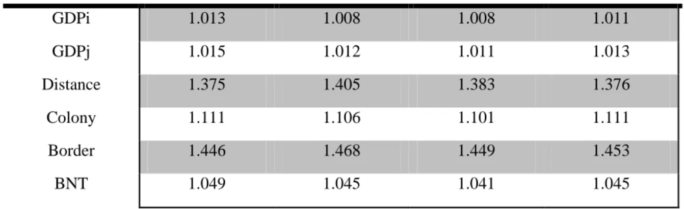
Table 4A: VIF statistics for the analysis of Baltic-Nordic Trade………- 32 -

Table 5A: VIF statistics for the analysis of Commodity Groups………- 32 -

Table 6A: Cook’s Distance Test for Normality and Mahalanobis Distance.. test for outliers for the Baltic-Nordic trade………....- 35 -

Table 7A: Cook’s Distance Test for Normality and Mahalanobis Distance test for outliers for the commodity groups……….- 36 -

Appendices:

Appendix A: The list of 42 European countries… ………..….- 26 -

Appendix B: The Descriptive Statistics………..- 27 -

Appendix C: The Regression Results………....- 29 -

- 1 -

1

Introduction

The environment for international trade has changed dramatically in the last decades: not only the volume of international trade has increased by a great extent but also the trade flows have been widely liberalized. Feenstra (1998) suggested four possible factors to explain the growth of the world trade: trade liberalization, falling transportation costs, convergence of economies and increased outsourcing. The outsourcing was caused due to the fact that international firms became more vertically specialized making the interme-diate goods to cross borders more times which led to an increase in trade relative to out-put.

The year of 1991 was crucial not only to the Baltic States (Estonia, Latvia, Lithuania) be-cause of gained independence from the Soviet Union but also for the rest of the European Continent. The new economies, including the Baltic States, were in the process of forming from centrally planned economies to market economies. Nevertheless, the trans-formation had a rough beginning; during the years of 1992-1994 the economic decline was obvious in all three Baltic countries. In the later years the accession to the EU fa-vored the economies of Baltic States’ by removing trade barriers, reducing transaction costs and shifting trade flows towards the EU markets.

During the communist period in the former Soviet Union, in Eastern Europe, including the Baltic States, the explicit goal for economy policy was the eagerness to limit any economic dependence on the Western economies. Thus, after the Baltic States had gained their independence, it was expected to lead to a major increase in the value of trade flows with the developed Western market economies (Hamilton, Hughes, Smith and Winters, 1992). Since the trade takes place only if the both trading partners believe that it will in-crease their welfare, it can be concluded that the Baltic States and the Nordic Countries had strong confidence in expectations of an increasing trade flows. This had a major im-pact not only on the Baltic States and other reforming economies but also on their new trade partners that had market economies. Moreover, trade is also seen as a primary in-strument to catch up with the established Western market economies. Therefore, opening the way for trade was one of the prime steps taken in the transition process in economies of Baltic States’. Economies with much more opened features attracted the flow of new and better technology through trade and foreign investment (Bergstrand, 1989). There-fore, the Baltic States increased their productivity levels and shifted the production to more sophisticated goods. The pattern of trade shifted from low valued goods and ser-vices to more costly commodities.

The breakup of planned economies for the Baltic States opened the way for trade liberali-zation, which was a major reform that was expected to bring the economic prosperity and future economic growth. The trade with the Nordic countries - Denmark, Finland, Nor-way and Sweden - had been the starting point for the Baltic States to penetrate into inter-national trade. Both groups of countries shared similarities in culture, climate, landscape, natural resource endowments, being geographical neighboring countries as well as shar-ing the coastline of the Baltic Sea. The economic situation includshar-ing the trade flows was of a great importance to both regions. This was reflected in the establishments of various organizations and institutions such as the Council of the Baltic Sea States. Furthermore,

- 2 - the Nordic countries adjusted their political and economic collaboration to the Baltic States after the dissolution of the Soviet Union.

Table 1 shows the exports from the Nordic countries to the Baltic States. Unsurprisingly, the exports were gradually increasing, however, there was a slight decline from 2006 to 2010. Finland showed the least growth (only 47%) while Norway increased its exports to the Baltic States by almost 280%. This visibly indicates that the economies of Baltic States became more open to imports and the importance of Nordic countries as an im-porting partner increased.

Table 1 Exports to the Baltic States, millions of current US dollars

1996 2001 2006 2010 Growth 1996 to 2010 Denmark 361 480 1005 735 104% Finland 1481 1444 3262 2171 47% Norway 156 169 470 591 279% Sweden 616 859 2301 2256 266% Source: UN Comtrade

Table 2, on the other hand, displays the imports to the Nordic countries from the Baltic States. The growth in imports was more significant than in exports suggesting that trade of the Baltic States became more liberalized. This clearly points out that the share of ex-ports of the Baltic States increased by a huge amount from 1996 to 2010. The growth percentages differ according to each of the Nordic Countries, but the Norway’s increase by 916% is worth mentioning. Although the numbers display huge growth, it is hard to tell from these figures if the Nordic countries were an important trading partner to the Baltic States. The analysis will reveal if this increase in bilateral trade between two re-gions was significant in the bilateral European exports context.

Table 2 Imports from the Baltic States, millions of current US dollars

1996 2001 2006 2010 Growth 1996 to 2010 Denmark 259 565 958 1102 326% Finland 434 1200 1866 2248 418% Norway 119 256 857 1209 916% Sweden 876 1254 2333 3245 270% Source: UN Comtrade.

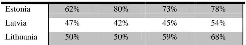
As the Table 2 showed the high increase in exports from the Baltic States to the Nordic Countries, it is interesting to look at the change of the exports as a percentage of GDP for the Baltic States. Table 3 represents the exports (% of GDP) which shows the value of all provided goods and services to the rest of the world. The exports (% of GDP) were pro-gressively increasing during the years for all States, especially Lithuania displayed growth by 18% between 1996 and 2010. The increase in the numbers also reveals that the

- 3 - trade became more central in the national policies, therefore the economies of the Baltic States became more open towards the rest of the world. It is typical for small countries like the Baltic States to have higher numbers in exports (% of GDP) than larger countries as minor economies incline to show larger participation rate in the international division of labor. Once again, Lithuania had the highest growth in share of participation compar-ing to Estonia and Latvia in 2010. As small economy’s size is not sufficient to support the higher levels of specialized production, its exports should increase. It can be seen that it was the case for all Baltic States.

Table 3 The exports as a percentage of GDP

1996 2001 2006 2010

Estonia 62% 80% 73% 78%

Latvia 47% 42% 45% 54%

Lithuania 50% 50% 59% 68%

Source: World Bank.

1.1 Purpose

The thesis aims to investigate the trade intensity between the Baltic States and the Nordic countries by examining the bilateral export flows between 42 European countries1 at 4 different years: 1996, 2001, 2006 and 2010. This is made by introducing the dummy for the Baltic-Nordic trade in order to observe how the direction and magnitude of this trade changes over time. The starting point is the year of 1996 due to the data availability and then the period of every 4-5 years should be sufficient to display the changes over time. Furthermore, the impact of differently valued commodities is taken into consideration to detect whether low, medium or high valued commodities had strongest impact on trade between the Baltic States and the Nordic countries over 14 years.

1.2 Outline of the Thesis

Having introduced the problem of this thesis, the historical background in presented in Part 2. In the following part, number 3, the theoretical framework is developed which provide more details about the gravity model application as well as geographical transac-tion costs. The fourth part is called empirical framework where the novel way of gravity model equation has been developed to investigate the bilateral exports in Europe with the focus on the Baltic States and the Nordic countries. The description of variables are pro-vided with the general summary of the descriptive statistics. Moreover, the hypotheses are presented there. The results of the regressions are displayed and the analysis of test-ing the hypotheses are given in Part 5. The main findtest-ings and the discussion are included in Part 5. In the last part, the conclusions are drawn in order to summarize the paper. The areas that need to be studied more in depth, and raise us more questions but have not been analyzed in this study, are listed after the conclusion.

- 4 -

2

Historical Background of the Gravity Model

Various forms of gravity model have been used in order to examine the trade flow pat-terns between the Baltic States and the Nordic countries. The most appealing and worth mentioning researches have been summarized below where the general form of gravity model was approached by exclusive techniques.

Byers, Isçan & Lesser (2000) used the gravity model in order to investigate the trade flows of the Baltic States after the breakup of the Soviet Union. Quite a strong assump-tion was made to predict the trade flows: in the absence of the Soviet occupaassump-tion the Bal-tic States were expected to follow the similar development pattern as the Nordic coun-tries did during the years of 1940-1990. Moreover, Byers, Isçan & Lesser (2000) estimat-ed the coefficients of the Nordic countries for the gravity model and then usestimat-ed them for the Baltic States to measure the potential trade flows. Two main conclusions for the Bal-tic States’ trade were made: the volume of trade had a sharp decline just after the gained independence (1993-1994) with a sudden increase in the following years; the trade flows shifted towards the EU countries as well as other Western economies. There have been similar approaches to predict the trade of the Baltic States where the unique difference is the novel way of calculating the gravity model parameters. For example, Borsos and Erkkila (1996) used the Baltic trade and income data, Wergeland (1997) employed the average of Western Europe or Baldwin (1994) looked at the Central and Eastern Europe-an countries. Although it is hard to compare these different approaches, one conclusion has been drawn: the trade flows shifted towards the West.

Hacker and Johansson (2001) analyzed the trade flows in the Baltic Sea region using the gravity model, with the variables that reflect the transaction costs, in order to expose the trade affinities between trading partners. The transaction costs are defined as

“transac-tion costs comprise resource consump“transac-tion when property rights are transferred between two agents (from buyer to seller)” (Hacker and Johansson, 2001, p.76). The concept of

the gravity model itself states that the cost of transaction diminishes as the distance be-comes shorter and/or the difference in trading characteristics such as language, culture, taxes or laws becomes larger. In their analysis Hacker and Johansson (2001) applied five dummy variables to reflect the trade affinities in social, geographical, and cultural con-cepts. The study revealed the existence of strong affinity between the Baltic States and Nordic countries.

For the analysis of the trade flows of the Baltic Sea region countries Paas (2002) adopted the gravity model and especially emphasized its usage “particularly in conditions of

in-terdependence between transition and integration processes of countries with different economic and political background. The latter is a typical feature of the Baltic Sea re-gion” (Paas, 2002, p.28). According to his research, the Baltic Sea region countries trade

swings in favor of a larger size economies or in other words with economies having higher GDP. Furthermore, trading inside the EU was proved to have the positive effect on the trade flows. The results of the gravity model in this analysis also indicated the ex-istence of high trade potential between the Baltic States and Scandinavian countries. In the study by Laaser and Schrader (2002) the changing trade patterns of the Baltic States were analyzed using the unique approach to the gravity model. The authors em-phasized the importance of the Russian transit trade, passing through the Baltic States,

- 5 - which positively contributes to the Baltics’ trade flows and suggested “the Baltic States

could serve as a bridge between the two Europes, having the stronger per on the western shore” (Laaser and Schrader, 2002, p.45). Although the gravitational power is not in

place to its full extent, the trade flows of the Baltic States tend to move in that pattern which characterizes the trade relations. The concluding idea of the study was the strength of the Baltic States trade links with the Scandinavian countries.

After introducing different studies in the examination of trade flows patterns, it can be observed that there are still some unanswered questions and therefore space for further research about the trade between the Baltic States and the Nordic countries.

- 6 -

3

Theoretical Framework

The trade is said to take place only if both trading parties believe it would increase their welfare. Being the main reason for trade, it is worth mentioning that countries are differ-ent from each other and therefore trade provides countries with the opportunity to ex-change of these differences and take benefit of it. Moreover, countries do trade to gain from the benefits of the economies of scale in production which expands the market area. Scale economies takes place when the countries specialize in the production of goods that they are relatively better in and thus are able to produce at a larger scale with lower costs than other countries would. Such specialization results in having the comparative ad-vantage in production of those goods. This efficiency for a country with a comparative advantage leads to sell these goods at a lower price which causes an increase in the de-mand for that particular good. Furthermore, the benefits from trade become present when the country export the goods that it produce more efficiently and import the goods for which it experience higher production costs (Krugman and Obstfeld, 2006).

It is necessary to build the theoretical framework for this analysis, more precisely, to in-troduce the gravity model and transactions costs. They are discussed in the following subsections.

3.1 The Gravity Model

The basics of the gravity model goes back to the Newton’s Law describing the force of gravity. For the first time to use gravity model for international trade was made by Tin-bergen 1962 and Linnemann 1966. Since then various approaches of the basic gravity models have been widely used in the empirical studies to investigate the changes in in-ternational trade patterns and therefore gained its popularity (see Wang Winters, 1991, Hamilton and Winters 1992, Baldwin 1994). Moreover, it is still at the center of applied research in international trade even after forty years of history. “The model explains the flow of trade between a pair of countries as being proportional to their economic “mass” (national income) and inversely proportional to the distance between them.” (Batra, 2006) .

Although, the gravity model has a strong empirical justification dating back to 17th centu-ry (Tinbergen, 1962; Pöyhönen, 1963) theoretical foundations have been debated. Figure 1 provides a broad picture of the theoretical path for the gravity model.

- 7 - Figure 1 The Theoretical Foundations of The Gravity Model

Classical Trade Theory Modern Trade Theory Comparative advantage Economies of Scale

Perfect Competition Product Differentiation The Heckscher-Ohlin Theorem Imperfect Competition

The ‘missing link’ Anderson (1979) Deardorff (1995) Bergstrand (1985 and

1989),Helpman and Krugman (1985)

Source: Iversen (2002)

It can be seen that there are two rather different approaches to the gravity model: one from the classical trade theory based on a comparative advantage; and another originating from the modern trade theory with the economies of scale where the comparative ad-vantage is seen in a more dynamic perspective. The classical trade theory assumes perfect competition in the market, where the economies of scale are absent, comparative ad-vantage and the Heckscher-Ohlin (H-O) Theorem plays important role. On the other hand, the modern trade theory is based on economies of scale, product differentiation and imperfect competition.

Starting from the classical trade theory, the comparative advantage in the H-O Theorem is seen as ‘a gift of nature’ since the production of the goods that a country has a compar-ative advantage requires to consume relcompar-atively abundant factor. However, the H-O theory did not explain the bilateral trade flows when there are no transfer costs.

Moving to the modern trade theory, Helpman and Krugman (1985) made a few very im-portant assumptions such as economies of scale, product differentiation and imperfect competition. These factors gave another approach to the gravity model. In order to combine these two points of views into one, further research was needed. That’s where Anderson (1979), Bergstrand (1985 and 1989), Helpman and Krugman (1985) and later Deardorff (1995) gave the extra-ordinary contribution to the theoretical foundations of the gravity model.

Deardorff (1995) proved the compatibility of the gravity model with modern trade theory as well as with the Heckscher-Ohlin Theorem. This relation between two theories has been approved as the most comprehensive theoretical contribution for the gravity model and therefore it is named as a ‘missing link’ (see Figure 1) by Iversen (2002). Further-more, in his later research Deardorff (1998) further developed this compatibility and

The Gravity Model Xij = αYi β1 Yj β2Dij β3

- 8 - ed that both the classical trade theory and modern trade theory fit together in modern general equilibrium theory where monopolistic competition and differentiated products do not contradict themselves. Finally, this model provides good analysis of trade flow patterns for the long run equilibrium (Nilsson, 2000).

The most basic form of the gravity model is:

Xij = αYi β1 Yj β2Dij β3 (2.1)

Or expressed in a linear function as:

ln(Xin) = α+ 1ln(Yi) + 2ln(Yj) + 3ln(Dij) (2.2)

Xij represents the trade value between a country i and country j, Yi stands for the “economic size” that is usually measured as a GDP value for a country i. Yj intuitvely is GDP for a country j and Dij shows the distance between two trading partners. Hence the trade flow between two trading agents are expected to be proportional to each country’s GDP and to diminish as the distance becomes larger.

Basically, the main idea of the gravity model is that large economies tend to have higher incomes and therefore can produce more goods and services. Furthermore, this leads for large economies to have higher spending levels on imports (Krugman and Obstfeld, 2006).

3.2 Geographical Transaction Costs

It would be naive to think that the countries trade without experiencing any costs, there-fore, the geographical transaction costs are introduced in this analysis. The definition of geographical transaction costs include all transport as well as transaction costs incurred in the bilateral trade. These expenditures occur when the property rights of particular good or service are moved from buyer to seller. In the gravity model, the geographical transactions costs is a proxy for distance variable that combines both components: trans-action and transportation costs and hence there is a positive relationship between the costs and distance (Johansson and Nilsson, 2001). Figure 2 shows the graphical way of presenting this link. Marimoutou, Peguin, and Peguin-Feiisolle (2010) interpret the tance as “an indicator of the cost of entry in a market (a fixed cost): the greater the

dis-tance, the higher the entry cost, and the more we need to have a large market to be able to cover a high cost of entry”.

The geographical transaction costs are expected to change between the various trading partners due to different geographical distances and explicit interaction links (Karlsson, Andersson, Cheshire and Stough, 2007). The expenditures tend to increase with longer distance that represents cultural differences which affect consumers’ preferences; and the way the business is done, e.g. trade restrictions or tariffs imposed by a government (Jo-hansson, 2000). The trade barriers, introduced in the gravity model by Anderson (1979) and Bergstrand (1985) are imposed in order to protect the domestic economy but it caus-es the volume of trade to diminish as well. Moving to the relationship between the differ-ently valued commodities and transaction costs, the value has contradicting effects on the geographical transaction costs. The high valued commodities are small in magnitude but large in value, thus they have positive link with the transaction costs. They can be traded

- 9 - at longer distances since the transportation costs takes rather small part of the particular commodity price. On the contrary, the low valued goods and services are large in size but small in value causing the negative impact on geographical transaction costs. It is obvi-ous that the distance becomes less important when the expensive goods and services are traded than comparing with cheaper commodities. However, usually higher valued goods require more face to face contact which tend to increase the price making them more dis-tance sensitive.

Figure 2 Transaction Costs

Geographical Transaction Costs

Transaction Costs

Distance Source: Hacker and Johansson (2001)

The Figure 2 represents the positive relationship between distance and geographical transaction costs. The geographic transaction costs tend to diminish when the distance between two trading partners is decreasing. The breaking points in the curve represent the transaction barriers for trade that usually occur at the borders, therefore the curve does not have a smooth path as it would be normally expected. It follows that trading agents having a short distance between them share lower costs and fewer trading barriers than agents with larger distance. On the other hand, there might be significant cost differen-tials at different sides of borders (Hacker and Johansson, 2001). Furthermore, Carlton and Perloff (2005) argued that the countries become more similar when the transaction costs diminish.

The transport costs determine the price wedge between the production cost at a domestic country and sales price in a foreign country and therefore define the demand for globally traded goods. (Steininger, 2001). Samuelson (1952) was first to introduce the transport sector into the trade models. Generally, the transport costs are modeled according to the iceberg model which says that transport consumes a fraction of the goods sold.

- 10 -

4

Empirical Framework

In this part of the thesis the models for the analysis are presented including the descrip-tion of all variables and dummies. The summary of descriptive statistics and hypotheses are stated in the following sub sections to provide with the full explanation of the empiri-cal model.

4.1 Data and Model

The export data has been obtained from the UN Comtrade which has been widely used in estimating the gravity model. The total values of the bilateral exports are taken between each of the 42 European countries, making it as an export matrix. For the analysis of commodity groups, the commodities only on 5 digit level were gathered.

The Ordinary Least Squares (OLS)2 method is used to investigate the bilateral exports between the Baltic States and the Nordic Countries and explore the value of commodities traded. In the first part, the bilateral exports of 42 European countries are investigated by introducing a dummy variable for the Baltic-Nordic trade to check its impact between these two regions. Furthermore, the dummies for common border and colonial ties are in-cluded in the analysis as well. The model is analyzed at four different years (1996, 2001, 2006 and 2010), which gives the period of 14 years. This time period should be sufficient to provide comprehensive analysis with satisfying results. The year of 1996 was chosen as a starting point due to the data availability and then every 4-5 years, which should clearly indicate any modifications of the impact.

Using a large number of dummy variables could lead to multicollinearity, in order to avoid it, it is necessary that there is no overlap between the categories defined by dummy variables. “ as categories of higher than average flows are dummied out, the coefficients

on GDP and distance become smaller, causing the model’s base to be lower” (Christie,

2002). Therefore, only three dummy variables are used in the analysis of the Baltic-Nordic trade and two dummies in testing the commodity groups.

The second model is introduced in order to get the further analysis of the Baltic-Nordic trade. The exports between the Baltic States and the Nordic Countries are taken on 5 digit level to investigate the impact of differently valued commodities traded for 1996, 2001, 2006 and 2010. Thus it will show if there is a pattern over time and how the value of commodities changed in 14 years. The dummy variables (LVC, MVC and HVC) are in-troduced in the second model to account for the low and high valued commodities, leav-ing the medium valued products as a benchmark.

4.2 Variables

Dependent variable:

Export, EX, is the dependent variable in the regression equation that represents all sold

goods and services in a country’s economy. The exports were chosen instead of imports

- 11 - as export values are reported as Free on Board (FOB) whereas imports are stated on the basis of Cost, Insurance, and Freight (CIF). This fact constitutes that in the import data transport costs are added to the domestic price of importing country and therefore causes to have greater and misleading values than export values. The export values are measured in billions of current US dollars. The data for exports were collected from UN Comtrade.

Independent variables:

Gross Domestic Product, Y, is an indicator of the value of all officially recognized

goods and services produced in a country at a particular time and reflects a country’s economic size. Countries with higher income tend to have higher trade flows than lower income countries due to more developed transportation infrastructure, lower tariffs etc. (Head, 2003). GDP of exporting country indicates a country’s supply capacity while GDP of importing country reflects the market potential of importing country. The varia-ble is measured at purchaser’s price instead of being estimated in Purchasing Power Pari-ty (PPP) as PPP tends to be biased and could lead to the overestimation of the exports (Gros and Gonciarz, 1996). According to Christie (2002): “trade usually happens at

in-ternational prices, and therefore GDP at PPP has no bearing in trade levels”. Normally

it is expected for the GDP to have a positive effect on exports (Bade and Parkin, 2004). GDP is estimated in billions of current U.S dollars converted from domestic currencies using the single year official exchange rate. The data were collected from World Bank.

Distance, D, is the other explanatory variable in the regression function and has been

proved to have relatively strong negative effect on trade relations in the gravity model. The distance represents the transport and transaction costs and therefore has a negative relationship with the trade flows. Thus the closer the countries are, the smaller the trans-actions costs occur due to better information and cultural similarities (Nilsson, 1999). It has been proved that the trade flows are expected to decrease by one half when the dis-tance doubles by conducting the analysis from 595 regressions functions in order to measure the significance of a distance as an explanatory variable in the gravity model (Head 2003). The specific way of measuring distance has been used in this paper since the variable was specially designed for the gravity literature by Mayer and Zignago (2011) with a wide range of gravity variables for all countries in the world. They calcu-lated the distances between two countries based on “bilateral distances between the

big-gest cities of those two countries, those inter-city distances being weighted by the share of the city in the overall country’s population”. The data for distance was gathered from

CEPII (2011).

Dummy variables:

Border, B, implies that the countries share the same border. It has been included in the

analysis in order to investigate if the neighboring countries tend to have greater trade in-tensity and thus it is expected to have the positive effect on exports (Hacker and Johans-son 2011). The common border is assumed to exist only when two countries share the border by land. That is, if there is the Baltic Sea separating two countries, they will not have the common border e.g. Sweden and Lithuania. The dummy is equal to 1 when two countries share the same border and 0 otherwise. The data was collected from CEPII (2011).

- 12 -

Colony, C, represents the colonial relationship between two countries that also captures

cultural and political ties. It includes any colonial links that ever existed between the countries with no respect to the history time. It has the positive sign since colonial link-ages are expected to increase the value of exports. According to Eichengreen and Irwin (1998), the colonialism can even cause a permanent effect on trade that cannot be ex-plained by other factors. The dummy is equal to 1 if two countries shared the colonial re-lationship and 0 otherwise. The data was obtained from CEPII (2011).

Baltic-Nordic trade, BNT, is the dummy variable that stands for the trade between

Nor-dic countries and Baltic States. It was introduced in the analysis in order to investigate if the bilateral exports between these two groups of countries were significant over the years in the context of Europe. The dummy equals 1 when the trade takes place between one of the Baltic States and one of the Nordic countries and 0 otherwise. The data col-lected from UN Comtrade.

Low valued commodities, LVC, is a dummy that accounts for the low valued

commodi-ties trading between two agents. The 5-digit level export data for the corresponding year was used to calculate the value of commodities. In order to get the value per one unit on-ly commodities measured in kilograms were chosen. This dummy is expected to have a positive sign. The low value commodities accounts for the 30 per cent of total commodi-ties with the lowest values. The dummy is equal to 1 when the products fall in the group of low valued and 0 if not. The data to calculate this dummy were used from UN Comtrade.

Medium valued commodities, MVC, is a dummy variable that represents the medium

valued commodities. It accounts for 40 per cent of total commodities with medium value. This dummy is a benchmark category in the regression model, thus, all conclusions that will be drawn in later sections will have medium valued commodities as a reference. The dummy equals to 1 when the commodity falls in the category of medium value and 0 otherwise. The data for this dummy was also collected from UN Comtrade.

High valued commodities, HVC, is a dummy which represents high value commodities.

The value of the commodities has been calculated in the same way as a dummy for low value commodities. High value commodities represents the 30 per cent of total commodi-ties with the highest values. These dummies for differently valued products were intro-duced in the analysis in order to account for different values. The dummy is expected to have negative relationship with the bilateral exports. The variable is equal to 1 when the commodity is high valued and 0 if not. The data for this variable were gathered from UN Comtrade.

4.3 Gravity Model Equation

By using the basic gravity model the following equations were constructed for this analy-sis to estimate the effects of selected variables on the bilateral exports. The exports are regressed on exporter’s GDP, importer’s GDP and distance; expecting the positive coef-ficients on both GDPs and negative for the distance.

- 13 - The log-linear models are:

ln(EXij)=lnα+β1ln(Yi)+β2ln(Yj)+β3lnDij+β4Bij+β5Cij+β6BNTij+εij (3.3.1.) ln(EXij)=lnα+β1ln(Y_i)+β2ln(Yj)+β3lnDij+β4LVCij+β5HVCij+εij (3.3.2.) where,

EXij = the value of exports between country i and country j ; Yi = the gross domestic product of exporting country i ; Yj = the gross domestic product of importing country j ; Dij = the distance between country i and country j ;

Bij = dummy variable having the value 1 if i and j share common border and 0 otherwise;

Cij = dummy variable having the value 1 if i and j have ever had a colonial ties and 0 otherwise;

BNTij = dummy variable having the value 1 if i is one of the Baltic States and j is one of the Nordic countries or vice versa and 0 otherwise;

LVCij = dummy variable assuming the value 1 if the value of commodities is low and 0 otherwise;

HVCij = dummy variable assuming the value 1 if the value of commodities is high and 0 otherwise;

εij = is an error term, assumed to be normally distributed.

4.4 Hypotheses

Hypothesis 1: The intensity of bilateral exports trade between the Nordic countries and the Baltic States have increased over 14 years. The relations between the European ex-ports and Baltic-Nordic trade are higher in 2010 than in 1996.

Hypothesis 2: The trade intensity of high value commodities have increased in the Baltic-Nordic trade due to the technological advances. That is, the trade in low value commodi-ties diminished over time.

4.5 Descriptive Statistics

The complete descriptive statistics can be found in the Appendix B. Table 2A consists of the regressions for the Baltic-Nordic trade and the Table 3A shows the descriptive statis-tics for the regressions of the commodity groups. Both tables contain the information of the mean, minimum, maximum, standard deviation and number of observations for each variable.

- 14 - Table 2A, shows that the mean values for the respective variables do not change much during the years. There is just a slight increase in all variables. For instance, the mean of the dependent variable (exports) increased only by 0.4 from 1996 to 2010. Both variables of GDPs also show the growth which had been expected as the GDP of a country is con-stantly growing. There is high standard deviation for the dependent variable which can be explained by the fact that prices of traded goods do vary. On the other hand, the deviation is rather low for the other variables: distance, GDP of exporter and GDP of importer. As the analysis is made of the European countries, it is not surprising that these variables are not far from their means. Although there are some differences in the European econo-mies, the values of their GDPs are more or less close to each other.

Table 3A displays quite similar results as the previous table did. The means of the GPDs slightly increased during the years representing the growth in the economies of the Nor-dic countries and the Baltic States. On the contrary, the means of the dependent variable show a decrease by 0.603 from 1996 to 2010. Although it is a small decline, it represents that the value of traded goods had decreased. The goods traded between the Nordic coun-tries and the Baltic States had become the ones of lower values. There is high deviation of exports variable, which represents the great value variety of goods and services ex-changed between the two trading groups.

- 15 -

5

Regression Results

In this section of the paper results of the regressions are presented to determine the sig-nificance of the independent variables and the overall goodness of the model used. The full analysis is prepared in order to draw the conclusions about the bilateral exports be-tween the Baltic States and the Nordic countries.

The tests to check for multicollinearity, heteroscedasticity as well as normality were con-ducted and it showed that there is a problem of heteroscedascity in the sample data. However, this phenomenon is commonly found in the gravity model analysis with cross-sectional data. The tests are summarized in the Appendix D.

5.1 Results for the Baltic-Nordic Trade

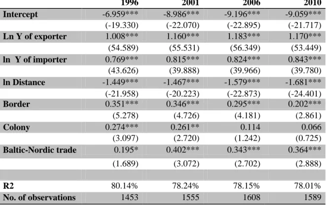
Table 4 summarizes the results of the OLS regressions for the 42 European countries’ bi-lateral exports at four different years: 1996, 2001, 2006 and 2010. The estimated parame-ter coefficients are provided in the tables and the t-statistic are given in the parentheses for each variable in order to present the strength and direction of influence. The signifi-cance level for each coefficient is illustrated by a respective number of asterisks. The last two rows show the R squared value and the number of observations for each regression. Table 4 Regressions Results for Baltic-Nordic Trade

1996 2001 2006 2010 Intercept -6.959*** -8.986*** -9.196*** -9.059*** (-19.330) (-22.070) (-22.895) (-21.717) Ln Y of exporter 1.008*** 1.160*** 1.183*** 1.170*** (54.589) (55.531) (56.349) (53.449) ln Y of importer 0.769*** 0.815*** 0.824*** 0.843*** (43.626) (39.888) (39.966) (39.780) ln Distance -1.449*** -1.467*** -1.579*** -1.681*** (-21.958) (-20.223) (-22.873) (-24.401) Border 0.351*** 0.346*** 0.295*** 0.202*** (5.278) (4.726) (4.181) (2.861) Colony 0.274*** 0.261** 0.114 0.066 (3.097) (2.720) (1.242) (0.725) Baltic-Nordic trade 0.195* 0.402*** 0.343*** 0.364*** (1.689) (3.072) (2.702) (2.888) R2 80.14% 78.24% 78.15% 78.01% No. of observations 1453 1555 1608 1589

*** significant at the 1% level, ** significant at the 5% level, * significant at the 10% level Dependent variable: ln Exports

- 16 - Most of the variables are statistically significant at 1% level, with only a few exceptions. For instance, the Baltic-Nordic trade dummy in 1996 and Colony dummy for 2006, 2010 display weak significance results. The usual dummies for gravity model estimation, the Border and Colony do not contradict with the theory showing the positive relationship with the bilateral exports. Their importance has been regularly decreasing over the years, which has also been previously expected.

Since the main focus is on the Baltic-Nordic trade, it is gladly to see that this dummy is significant over time with the strongest impact in the year of 2001. However, the value of estimate did not vary much during the years with the lowest value of 0.195 in 1996. From 2001 to 2010 it has remained almost the same which is 0.38. The first hypothesis that the Baltic-Nordic trade intensity has increased over time is confirmed since there is obvious increase in the coefficient of BNT dummy. An increase by one percent in the trade between these two regions causes for approximately forty percent increase in the European bilateral exports. The BNT dummy gives more strength to the European trade than the common border and colony do. Therefore, the BNT dummy is the most signifi-cant to the European trade than any other in this analysis.

The Y of exporter has stronger impact than Y of importer due to the higher coefficients. Since the former variable represents a exporting country’s supply capacity, it can be said that the European countries have increased their supply capacities. Both elasticities of Y are close to 1 indicating that one percent increase in Y leads to approximately the same percentage increase in exports.

The Distance variable has proved to be highly significant at all times and therefore goes in line with the theory of acquiring the negative impact on the bilateral exports. The larg-er the distance, the lowlarg-er the bilatlarg-eral exports. Moreovlarg-er, this coefficient has been gradu-ally growing over time, giving the idea that the magnitude of distance effect between the trading partners has increased. The closer countries, for instance Italy and Spain are be-lieved to have higher levels of bilateral exports than Italy and Denmark. Since the elastic-ity is more than one, approximately 1.5, the one percent increase in distance causes to decrease in the bilateral exports on average by one and a half percent.

The measure of “the goodness to fit”, R2, indicates of how well the sample regression line fits the data. The larger it is, the more percentage of total variation in bilateral ex-ports is explained by the model. Looking at the results in Table 4 this measure is around 80% which is plausible and, therefore, 80% of variation in bilateral exports in explained by the regressors (Y of exporter, Y of importer, distance) and dummy variables (colony, border and Baltic-Nordic trade).

5.2 Results for the Commodity Groups

Table 5 illustrates the OLS regressions for the 7 countries (4 Nordic countries and 3 Bal-tic States) bilateral exports at the same years used before. There are two dummy variables included in the analysis to account for the low and high valued commodities leaving me-dium valued commodities as a benchmark. The export data was disaggregated in order to get the values of commodities. They were disaggregated at 5 digit level of Standard In-ternational Trade Classification (SITC) system.

- 17 - Table 5 Regressions Results for Commodity Groups

1996 2001 2006 2010 Intercept -3.499 13.155*** -40.267*** -21.924*** (-1.311) (4.543) (-11.857) (-6.230) ln Y of exporter 0.393*** 0.127** 1.184*** 0.832*** (6.835) (2.046) (16.759) (11.476) ln Y of importer 0.299*** -0.136** 1.0158*** 0.550*** (5.167) (-2.173) (14.339) (7.532) ln Distance -0.559*** -0.564*** -0.865*** -0.605*** (-19.956) (-19.374) (-26.153) (-13.586) LVC 0.053 -0.008 0.259*** 0.605*** (1.153) (-0.170) (5.201) (10.430) HVC -0.109*** -0.217** -0.208*** -0.016 (-2.638) (-5.312) (-4.633) (-0.302) R2 4.18% 5.82% 4.40% 3.41% No. of observations 12420 18648 20064 15336

*** significant at the 1% level, ** significant at the 5% level, * significant at the 10% level Dependent variable: ln Exports

Most of the estimators are significant at 10% level or less, however, there are a few cases where the estimates were not statistically significant. For instance, LVC at 1996 and 2001, HVC at 2010.

The variables representing the economic size of a country, the Y of exporter and Y of importer show similar results as in previous regressions. Interestingly, in 2001 the Y of importer had negative effect on the bilateral exports. On the contrary, the strongest im-pact was observed in 2006. The elasticity varies from -0.127 to 1.184 indicating that the Y had different impacts over the years.

The distance variable has negative links but does not show any increasing or decreasing trend over time. The lowest coefficient of -0.865 is in 2006 saying that in the year of 2006 the increase in distance had strongest negative impact on the bilateral exports. Thus, Estonia and Norway is believed to have less trade than Finland and Estonia.

The low value commodities are expected to have positive links with the bilateral exports since they are large in size but small in value. Looking at the Table 5, it can be nearly confirmed, as the LVC dummy has positive sign for all years, except 2001. However, the LVC coefficient in 2001 is rather low, almost equal to zero, having nearly nil effect on the Baltic-Nordic exports. There is a tendency in lower valued commodities since the co-efficients of 2006 and 2010 have been increasing.

The hypothesis number two cannot be approved here, since there is no obvious increase in trade of high valued commodities. Surprisingly, the coefficient of HVC is not even sta-tistically significant in 2010. It can be concluded that there was no difference in trade in high or medium valued commodities. However, as the theory suggested that there should

- 18 - be negative links between the high valued goods and services and the bilateral exports, it can be supported due to the negative signs of HVC coefficient.

The R2 is rather low for all regressions, however, the analysis is done only for 7 countries which can be one of the reasons why this measure does not acquire high values. Moreo-ver, it is rather common to have low R2 in the social sciences, especially in the cross sec-tional analysis with low variation in the data. The number of observations varies for each year, 2006 has the highest number of observations (more than 20 thousands).

5.3 Analysis

The results shown in previous sections revealed that almost all of the independent varia-bles have statistically significant impact on the bilateral exports. The Y of both exporter and importer have positive relationship and the distance has relatively strong negative impact on exports. The distance has shown higher importance on the European exports than on the Baltic-Nordic trade. The commonly used dummies such as Border and Colo-ny go in line with the theory of having the positive effect on exports. However, their sig-nificance has decreased over time.

The variables of the high interest in this analysis are the dummies for the Baltic-Nordic trade and for low/medium/high value commodities. The expectation is that the trade in-tensity of Baltic-Nordic trade has increased over 14 years. The regression results confirm this and indicate that the magnitude of trade between those two regions is becoming more important in the European trade context.

The high increase of BNT coefficient from 1996 to 2001 can be explained by the geo-graphical transaction costs. After the Baltic States gained independence, the trade poli-cies were changed dramatically; the trade was widely liberalized. Although those trade policies opening up the trade were established in the first years of independence, their ef-fect is observed only by the year of 2001. Furthermore, BNT dummy is the most signifi-cant to the European trade in comparison to the common border or colony dummies and thus the trade between the Baltic States and the Nordic countries gives extra strength to the European trade.

The results of the second regression analysis, that is conducted to capture the impact of differently valued commodities show that the importance of value is much lighter than was previously expected. It is important to remember that all statements made about the low and high valued commodities are in comparison to the medium value since it is the benchmark category. The low valued commodities show a positive correlation with the Baltic-Nordic trade whereas the high value goods and services display the negative rela-tionship. The transportation costs for low valued commodities account for substantial part of the price which makes them being traded with short distance therefore they have higher tendency to trade. The trade intensity in low valued increased from 1996 to 2010 in the Baltic-Nordic trade. Since those two regions are rather close to each other, they do have more trade in low valued than medium valued commodities. The demand for high valued goods and services in the Baltic-Nordic trade has decreased whereas the demand for low valued commodities became higher in comparison to the medium value.

- 19 - The negative signs of HVC variable indicate that when the commodities are more expen-sive, it negatively affects the bilateral exports between the Nordic countries and the Bal-tic States. On the contrary, when the commodities are low valued, the exports between these two regions and LVC have a positive relationship. This is caused by the particular commodity group’s price. For instance, the transportation costs of high valued commodi-ty take a small proportion of that commodicommodi-ty price and thus the distance becomes less important. The opposite applies to the low valued goods and services. Therefore, there is higher trade intensity in low valued commodities than in high valued between the Baltic States and the Nordic countries. Although the hypothesis of increased trade intensity in high value commodities has been rejected, it is interesting to observe that the value does not play an important role in the Baltic-Nordic trade.

Normally, HVS are less distance sensitive since the geographical transaction costs ac-count for rather small part of their price. However, the high valued commodities usually require more personal contacts in order to finalize the deal. This necessity of face to face contact directly increase the value of particular commodity, therefore, high valued com-modities sometimes are more distance sensitive. There was higher demand for low val-ued commodities comparing with medium valval-ued in the Baltic-Nordic trade. By the same token, the demand of high valued goods and services decreased from 1996 to 2010. Due to the increasing coefficient of HVS, the high valued commodities became less distance sensitive in the Baltic-Nordic region.

The Y of exporter and Y of importer are coherent with the theory displaying statistically significant correlation with the bilateral exports. There are many previous studies that have shown a positive correlation between Y and exports, for instance, Feenstra, Markusen and Rose 1999. The Y of exporter has higher values for all years than the Y of importer. It is worth mentioning that the Y of exporter captures the export supply of an economy, telling that higher Y increases the export supply and thus country’s exports are higher.

Marimoutou (2010) signified that larger Y of importer makes distance less significant obstacle to trade. The Y of importer has negative sign for 2001, indicating that an in-crease in a partner country’s Y resulted in decline in the bilateral exports. It is an interest-ing fact that has difficulty in givinterest-ing the appropriate explanations as it contradicts with the theory. Possibly that in 2001 the countries with lower Y had larger proportion of bilateral exports than higher income countries. The other estimators for the Ys are positive dis-playing the increase in the bilateral exports when the GDP grows. The European coun-tries with larger economic size tend to trade more.

The results of the distance variable do not contradict with the theory mentioned in the previous parts, since this variable has negative signs for all years. The increase in the dis-tance results in the decrease of the European countries bilateral exports. For insdis-tance, Portugal’s and Finland’s bilateral exports were not as high as Germany’s and France’s for all years. Moreover, in the European bilateral exports, the commodities became more distance sensitive comparing 1996 and 2010. When the distance between one of the Bal-tic States and one of the Nordic States increased, the bilateral exports declined. For all four years, the effect is almost the same, around 0.6., only in 2006 the distance had stronger consequence on the exports.

- 20 - According to the theory, the border variable implies lower transport costs, close cultural links that make trade less expensive between the trading agents. This dummy showed significance for all years which supports the theory that the bilateral exports of neighbor-ing countries, i.e. Spain and Portugal, were higher. Unsurprisneighbor-ingly, the significance of a common border has diminished during the years indicating that countries has increased trade with not neighboring partners. One of the reasons could be much lower transaction costs in 2010 than they were in 1996. If a country can benefit from trade with not neigh-boring trading partner, it will capture the opportunity whether they share a common bor-der or not. Very similar can be said about the impact of colonial ties on trade. Its effect is much lower in 2010 than it was 14 years ago. Overall, the world has become more glob-alized and the facts of common border or colonial ties do not play a huge role in making decisions to trade.

- 21 -

Conclusions

The thesis aimed to explore the trade intensity of the Baltic-Nordic trade in the context of the European bilateral exports over time. Although many previous studies highlighted the importance of trade between these two regions, now it is obvious that the trade intensity between the Baltic States and the Nordic countries increased from 1996 to 2010.

Although the impact of distance was not the main focus area of the analysis, it has been surprisingly to discover that the effect of distance on trade has increased over 14 years. The commodities traded in the European countries become more distance sensitive. Therefore, despite that the Europe is united and there are many trade agreements that aim to make the trade easier, the larger distance between the trading partners do lower the trade. Moreover, the magnitude of colony and common border effects on the bilateral export has substantially decreased.

After the analysis of the differently valued commodities, it can be concluded that the trade intensity in low/medium/high valued goods and services was changing over time. In 2006 and 2010 there was more trade in low valued than medium valued commodities in the Baltic-Nordic trade. As for the high valued commodities, since they are less distance sensitive, they had negative correlation with the exports. The trade in the expensive goods and services were not as high as in medium valued.

The analysis has revealed the increasing economic significance of the Baltic-Nordic trade and therefore it suggests the policy makers to pay more attention to those regions. The trade policies should be more oriented to those regions, since the trade intensity of the Baltic-Nordic trade has increased over the years.

One of the suggestions for further research on this topic would be to use panel data in-stead of cross-sectional data since it would provide more elaborate results. In the recent decade there have been various interesting analyses on the gravity model using different approaches, for instance, monte carlo simulation. It would be interesting to see how the results from this paper would differ between cross-sectional analysis and monte carlo techniques.

Another attractive idea is to make the analysis for other group of countries. For instance, to investigate the significance of trade between the former Soviet Union countries and Russia. When analyzing the trade in the Baltic-Nordic region, the other dummies could be introduced such as the dummy for trade only between Baltic States.

- 22 -

References

Anderson, J.E. (1979). A Theoretical Foundation of the Gravity Model. American

Eco-nomic Review 69, 1, 106-16.

Bade, R. and Parkin, M. (2004). Foundations of Macroeconomics (2nd ed.). Boston: Pearson Addison-Weasley.

Baldwin, R. (1994). Towards an Integrated Europe. Centre for Economic Policy Research, London.

Batra, A. (2006). India’s global trade potential: the gravity model approach. Global

Eco-nomic Review, 35(3).

Bergstrand, J. H. (1985). The Gravity Equation in International Trade: Some Microeco-nomic Foundations and Empirical Evidence. Review of EcoMicroeco-nomics and

Statis-tics, 67, 3, 474-81.

Bergstrand, J. H. (1989). The Generalized Gravity Equation, Monopolistic Competition, and the Factor-proportions Theory in International Trade. Review of Economics

and Statistics, 71, 1, 143-53.

Borsos, J., and Erkkila, M. (1996). Foreign Direct Investment and Trade Flows between the Nordic Countries and the Baltic States. In OECD, Regional Integration of

Transition Economics. Paris:OECD.

Byers, D. A., Işcan, T. B., and Lesser, B. (2000). New borders and trade flows: a gravity model analysis of the Baltic States. Open economics review 11: 73-91(2000). Carlton, W. D., and Perloff, M. J. (2005). Modern Industrial Organization (5th ed.).

Har-per-Collins. Boston: Pearson Addison-Wesley.

Christie, E. (2002). Potential Trade in South-East Europe: A gravity Model Approach. SEER-South-East Europe Review for Labor & Social Affairs, South-East Europe Review, 4, 81 – 102, Sofia.

Cook, D. (1977). Detection of Influential Observation in Linear Regression.

Technomet-rics, Vol. 19, No. 1, pp 15-18. Published by American Statistical Association

and American Society for Quality.

Deardorff, A. (1995). Determinants of Bilateral Trade: Does Gravity Work in a Neoclas-sical World?. NBER Working Papers 5377, National Bureau of Economic Re-search, Inc.

Deardorff, A. (1998). Determinants of Bilateral Trade: Does Gravity Work in a Neoclassical World?. In Frankel, J.A. (Ed.), The regionalization of the world

economy. (p.7-32). University of Chicaco Press: Chicago.

Eichengreen, B., and Irwin, D.A. (1998). The role of History in Bilateral Trade Flows. In Frankel J.A. (Ed.)., The Regionalization of the World Economy. The University of Chicago Press.

- 23 - Feenstra, R. C. (1998). Integration and Disintegration in the Global Economy. Journal of

Economic Perspectives, Fall, 31-50.

Feenstra, R.C., Markusen J.R., and Rosem A.K. (2001). Using the Gravity Equation to Differentiate among Alternative Theories of Trade. Canadian Journal of

Economics 34(2): 430-447.

Gujarati (2004). Basic Econometrics (5th ed.). Boston:McGraw Hill.

Gros, D., and Conciarz, A. (1996). A Note on the Trade Potential of Central and Eastern Europé. European Journal of Political Economy, 12 (4), 709-721.

Hacker, S., and Johansson, B. (2001). Sweden and the Baltic Sea Region: Transaction

Costs and Trade Intensities. In J.Bröcker & Herrmann H. (Eds.)., Essays in

Honor of Karin Peschel (p.75-85). Heidelberg : Physica-Verlag.

Hamilton B.C., Hughes G., Smith A., and Winters, A.L. (1992). Opening up International Trade with Eastern Europe. Published by: Blackwell Publishing. Economic

Pol-icy, Vol 7, No 17 (April 1992), pp 77-116.

Head, K.. (2003). Gravity for Beginners. Faculty of Commerce, University of British Co-lumbia, 2053 Main Mall, Vancouver, BC, V6T1Z2, Canada.

Helpman, E. And Krugman, P.R., (1985). Market Structure and Foreign Trade:

Increasing Returns,Imperfect Competition, and the International Economy.

Cambridge, MA: MIT Press.

Iversen, S.P. (2002). Handel, Transition og Integration.- Central- og Østeuropa og det tidligere Sovjetunionen. Artikler, essays, working papers og

konferencebidrag. Ph.Thesis no. 30/2002.

Johansson, B., and Westin, L. (1994). Affinities and frictions of trade networks. Re-trieved March 5th, 2008 from

http://www.springerlink.com/content/l506856415wt8150/fulltext.pdf

Johansson, B., and Nilsson, D. (2001). Trade and transport flows in the Baltic Sea region – Workshop in Copenhagen, September 2000. JIBS Working Paper Series, No. 2001-6.

Karlsson, C., Andersson, A.E., Cheshire, P. and Stough R.R. (2007). Innovation, Dynam-ic Regions and Regional DynamDynam-ics. CESIS, ElectronDynam-ic Working Papers, No. 89. Krugman, P.R. and Obstfeld, M. (2006). International Economics Theory and Policy.

(7th ed.). Addison-Wesley, Boston.

Laaser, K., and Schrader, C.F. (2002). European integration and changing trade patterns: the case of the Baltic States. Kiel Institute for the World Economy, Kiel

- 24 - Leamer, E.E. (1983). Model Choice and Speicification Analysis. Zvi Griliches and

Mi-chael D. Intriligator, eds., Handbook of Econometrics, vol I, North Holland Pub-lishing Company, Amsterdam.

Linnemann, H. (1966). An Econometric Study of International Trade Flows. Amsterdam: North Holland Publishing Company.

Mahalanobis, P.C. (1936). On the generalised distance in statistics. Proceedings of the National Institute of Sciences of India 2 (1): 49–55. Retrieved 2012-05-03. Marimoutou V., Peguin D., and Peguin-Feissolle, A. (2010). The Distance-varying

Grav-ity Model in International Economics: is the Distance an Obstacle to Trade?.

Economics Bulletin Volume 29, Issue2.

Mayer and Zignago. (2011). Notes on CEPII’s distances measures (GeoDist). CEPII

Working Paper 2011-25.

Neter, J., Wasserman, W., and Kutner, M. (1989). Applied Linear Regression Models. Boston, MA: Richard D. Irwin.

Nilsson, K.(1999). Alternative Measures of the Swedish Real Effective Exchange Rate.

National Institute of Economic Research Working paper No. 68, Stockholm

Nilsson, L., (2000). Trade integration and the EU economic membership criteria.

European Journal of Political Economy 16(4): 807-27.

Paas, T. (2002). Gravity approach for exploring Baltic Sea regional integration in the field of international trade. HWWA Discussion Paper, No. 180.

Peschel, K. (1997). Perspectives of regional development around the Baltic Sea. Institut fur Regionalforschung, Christian-Albrechts-Universitat zu Kiel, Olshausenstras-se 40, D-24098 Kiel, Germany.

Pöyhönen, P. (1963). A Tentative Model for the Volume of Trade Between Countries.

Weltwirtschaftliches Archiv, 90 (1),93-99.

Rogerson, P. A. (2001). Statistical methods for geography. London: Sage.

White, H. (1980). A Heteroscedasticity Consistent Covariance Matrix Estimator and a Direct Test of Heteroscedasticity. Econometrica, vol. 48., p 817-838.

Samuelson, P. (1952). The Transfer Problem and Transport Costs: The Terms of Trade When Impediments are Absent. Economic Journal 62, 278-304.

Steininger, K.W. (2001). International Trade and Transport: spatial structure and

envi-ronmental quality in a global economy. UK: Edward Elgar Publishing Limited.

- 25 - Wang and Winters (1991). The Trading Potential of Eastern Europe. CEPR Discussion

Paper 610.

Tabachnick, B. G., and Fidell, L. S. (2007). Using multivariate statistics (5th ed.). Boston: Allyn and Bacon.

Wergeland, T. (1997). The Future Trade Opportunities of the Baltic Republics. In T. Haavisto (ed.) The Transition to a Market Economy. Cheltenham, UK: Edward Elgar.

- 26 -

Appendix A

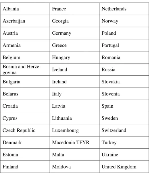
Table 1A: The full list of 42 European Countries included in the analysis for Baltic-Nordic Trade

Albania France Netherlands

Azerbaijan Georgia Norway

Austria Germany Poland

Armenia Greece Portugal

Belgium Hungary Romania

Bosnia and

Herze-govina Iceland Russia

Bulgaria Ireland Slovakia

Belarus Italy Slovenia

Croatia Latvia Spain

Cyprus Lithuania Sweden

Czech Republic Luxembourg Switzerland

Denmark Macedonia TFYR Turkey

Estonia Malta Ukraine

- 27 -

Appendix B

Table 2A: The Descriptive Statistics for the Baltic-Nordic Trade

Varia ble ln exports ln Y exporter ln Y importer ln

distance Border Colony BNT

1996 Mean 7.658 10.802 10.694 3.135 0.09 0.040 0.02 Min 2.777 9.229 9.229 1.775 0 0 0 Max 10.766 12.387 12.387 3.696 1 1 1 St. deviation 13.454 0.859 0.901 0.280 0.29 0.188 0.14 No. of Obs. 1453 1453 1453 1453 1453 1453 1453 2001 Mean 7.616 10.73 10.694 3.142 0.09 0.04 0.02 Min 1.279 9.170 9.170 1.775 0 0 0 Max 10.787 12.274 12.274 3.696 1 1 1 St. deviation 14.601 0.852 0.852 0.283 0.286 0.190 0.135 No. of Obs. 1555 1555 1555 1555 1555 1555 1555 2006 Mean 7.999 11.026 11.017 3.139 0.09 0.04 0.02 Min 1.602 9.533 9.533 1.775 0 0 0 Max 11.029 12.463 12.463 3.696 1 1 1 St. deviation 14.193 0.793 0.809 0.282 0.283 0.190 0.133 No. of Obs. 1608 1608 1608 1608 1608 1608 1608 2010 Mean 8.084 11.139 11.104 3.144 0.09 0.04 0.02 Min 2.646 9.764 9.764 1.775 0 0 0 Max 0.1392 12.156 12.156 3.696 1 1 1 St. deviation 14.017 0.759 0.785 0.281 0.283 0.191 0.134 No. of Obs. 1589 1589 1589 1589 1589 1589 1589

Table 3A: The Descriptive Statistics for the Commodity Groups

Variable ln exports ln Y exporter ln Y importer ln distance LVC HVC 1996 Mean 9.979 2.512 2.327 5.936 0.25 0.34 Min 6.217 22.277 22.277 4.394 0 0 Max 17.823 26.345 26.345 6.955 1 1 St. Deviation 20.279 1.486 1.456 0.843 0.43 0.47 No. Of Obs. 12420 12420 12420 12420 12420 12420 2001 Mean 9.556 2.478 23.89 6.056 0.25 0.33 Min 0.693 22.554 22.554 4.394 0 0 Max 19.729 26.150 26.150 6.955 1 1 St. Deviation 24.664 1.475 14.530 0.808 0.434 0.472 No. Of Obs. 18648 18648 18648 18648 18648 18648

- 28 - 2006 Mean 9.669 2.541 2.477 6.122 0.24 0.34 Min 0.693 23.545 23.545 4.394 0 0 Max 19.371 26.712 26.712 6.955 1 1 St. Deviation 28.200 1.301 1.301 0.797 0.428 0.474 No. Of Obs. 20064 20064 20064 20064 20064 20064 2010 Mean 9.376 2.542 2.517 6.328 0.24 0.34 Min 0.693 23.679 23.679 4.394 0 0 Max 18.1560 26.852 26.852 6.955 1 1 St. Deviation 28.555 1.371 1.322 0.606 0.428 0.474 No. Of Obs. 15336 15336 15336 15336 15336 15336