Training Risk Measure Models to Ascertain Which Continent’ Equity Has the Highest Risk ForInvestment Based On Randomly Selected Individual Continents’ Equities Listed On The New YorkStock Exchange

1 School of Education, Culture and Communication

Division of Mathematics / Applied Mathematics

MASTER THESIS IN MATHEMATICS / APPLIED MATHEMATICS

TRAINING RISK MEASURE MODELS TO ASCERTAIN WHICH CONTINENT’ EQUITY HAS THE HIGHEST RISK FOR INVESTMENT BASED ON RANDOMLY SELECTED

INDIVIDUAL CONTINENTS’ EQUITIES LISTED ON THE NEW YORK STOCK EXCHANGE

Author

EVELYN DELA GBADAGO

MASTERUPPSATS I MATEMATIK / TILLÄMPAD MATEMATIK

DIVISION OF MATHEMATICS / APPLIED MATHEMATICS

MÄRLARDALEN UNIVERSITY SE-72123 VÄSTERÅS, SWEDEN

2 School of Education, Culture and Communication

Division of Mathematics / Applied Mathematics

DIVISION OF MATHEMATICS / APPLIED MATHEMATICS

Master Thesis in Mathematics / Applied Mathematics Date: January 15, 2021

Project Name:

Training Risk Measure Models to Ascertain Which Continent’ Equity Has the Highest Risk For Investment Based On Randomly Selected Individual Continents’ Equities Listed On The New York Stock Exchange

Program:

Master’s Programme In Financial Engineering, 120 ECTS Credits Author:

Evelyn Dela Gbadago Supervisor: Lars Petterson Co-Supervisor: Linus Carlsson Reviewer: Richard Bonner Examiner: Achref Bachouch Comprising:

3

Abstract

Western countries, institutions, and people from all walks of land, including Africans, have carried the notion that it is riskier to invest in African countries compared to countries in other continents. This study verified if that notion is empirically established or it is just a mere notion born out of people's imagination and unfounded belief. The study did select one special metal mining company listed on the New York stock exchange from every continent using a systematic random sampling of period five. All these stocks' data were daily data spanning the period 2003-06 - 2020:06 obtained from Yahoo Finance. The said duration was used for the analysis because one of the companies selected for the study only had stock data starting from 2003-06-25.

Because of Generalized Autoregressive Conditionally Heteroscedastic (GARCH) ability to model the conditional randomly varying volatility, the study trained several of them for a different order of the GARCH terms σ2, and the order of the ARCH terms ε2 and for different distributions. Based on the AIC and BIC, the GARCH model that best fitted the data was GARCH (1,1), thus order one of the GARCH terms σ2 and order one of the ARCH terms ε2 based on student-t innovation. The study proceeded to estimate the risk measure using three of the approaches (risk metrics, Block Maxima Method under extreme value situation, and Generalized Pareto Distribution (GPD) for the tail ends of the distribution). None of the approaches or methods used in calculating VaR or conditional VaR (ES) of the stocks supported the conventional beliefs and age long-held purported gospel that African counties are the riskiest to invest on earth. In the risk metrics approach, the African stock was second riskiest to European stock. At the same time, in extreme value situations, it was third to European and South American; with GPD, it was third once again to South American and European stock. The study proceeded to verify if this founding were statistically significant. Applying analysis of variance (ANOVA), found that none of the differences established above is statistically significant. Meaning, statistically, the value and conditional value of one's investment that will be at risk is not different based on the investment's continental location. Thus, it is not statistically riskier to invest in one continent than the other.

Keywords: Continetal investment, New York Stock Exchange, Value-at-Risk, Special Metal Industry and Africa.

4

ACKNOWLEDGEMENT

My most tremendous gratitude goes to Almighty God for giving me the strength, courage, and guidance throughout the work. Completion of the thesis could not have been possible without the assistance of the following people: Anatoliy Malyareko for helping me with most of the mathematical methods, Augustine K. Osei-Fosu for his professional support and encouragement, Kofi Nyamekye, and Mr & Mrs. Korletey. I deeply appreciate their support and sincerely acknowledged it.

Lastly, to all families especially my Mum and Dad Mrs Florence Anim and Mr Dacusta A. Gbadago respectively, friends especially Abeba Gabrekidan, and others who assisted me in one way or the other with their support, physically, morally, and financially too, thank you.

Stockholm, January 2021. Evelyn Dela Gbadago

5

Contents

Abstract ... 3 ACKNOWLEDGEMENT ... 4 Contents ... 5 Table of Figures ... 7 Lists of Tables ... 8 CHAPTER ONE ... 9 Introduction ... 9 Background ... 9 Problem Statement ... 11 Research Question ... 12 Purpose ... 12 Significance ... 13 Rationale ... 13 Definition of Terms ... 14 Scope ... 15 Organization ... 15 CHAPTER TWO ... 16 Literature Review ... 16 Investment ... 16

Inadequate Investment in Africa ... 16

Reasons for Choosing a Place for Investment... 17

Types of Risk measure ... 18

Value-at-Risk (VaR) ... 18

Measuring Value-at-Risk ... 20

Variance-Covariance Method (VCM) ... 20

Historical Simulation (HS) ... 20

Monte-Carlo Simulation ... 21

6

Extreme Value Estimations ... 24

Extreme Value Theory for Peak Over Threshold Method ... 24

Expected Shortfall ... 26

Modeling the Return Distribution ... 27

ARCH Model ... 27

GARCH Model ... 32

IGARCH Model ... 33

Generalized Pareto Distribution ... 33

CHAPTER THREE ... 35

Methodology ... 35

Data and Variables Definitions... 35

Empirical Strategy ... 36

Unit root test ... 36

Chapter Four ... 38

Results and Analysis ... 38

Time Series Plot... 38

Model Selection ... 43

GARCH Model ... 43

CHAPTER FIVE ... 49

Conclusion, Findings, and Recommendations ... 49

Conclusion ... 49

Recommendations ... 50

Practical Limitation ... 52

Chapter six ... 53

Summary of reflection of objectives in the thesis ... 53

REFERENCE ... 55

Appendix 1 ... 62

Code ... 62

Appendix 2 ... 69

7

Table of Figures

FIGURE 2.1: GRAPH OF EXTREME VALUE DISTRIBUTIONS (SOURCE: JON DANIELSON (2017, P. 11)) 22 FIGURE 2.2: GRAPH OF EXPECTED SHORTFALL IN CONTRAST TO VAR (SOURCE: PORTFOLIO MASON

(2018)) 27

FIGURE 4.1: TIME SERIES PLOT OF ALL THE ADJUSTED STOCK PRICES 38

FIGURE 4.2: PLOT OF THE LOG DIFFERENCE OF THE ADJUSTED STOCK PRICES. 40

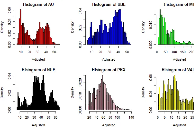
FIGURE 4.3: HISTOGRAM OF THE ADJUSTED STOCK PRICES. 41

FIGURE 4.4: HISTOGRAM OF LOG RETURNS OF THE ADJUSTED STOCK PRICES. 41

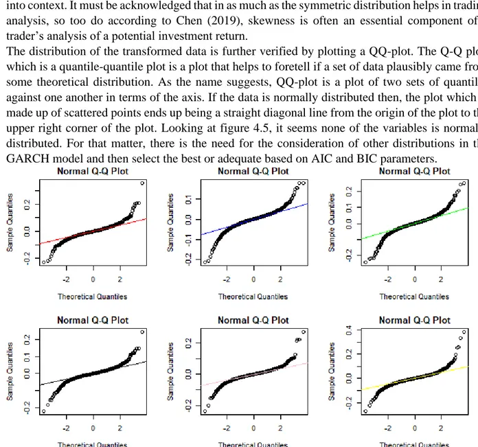
FIGURE 4.5: NORMAL QQ-PLOTS 42

8

Lists of Tables

TABLE 3.1 INFORMATION ON SELECTED COMPANIES FOR THE STUDY 36

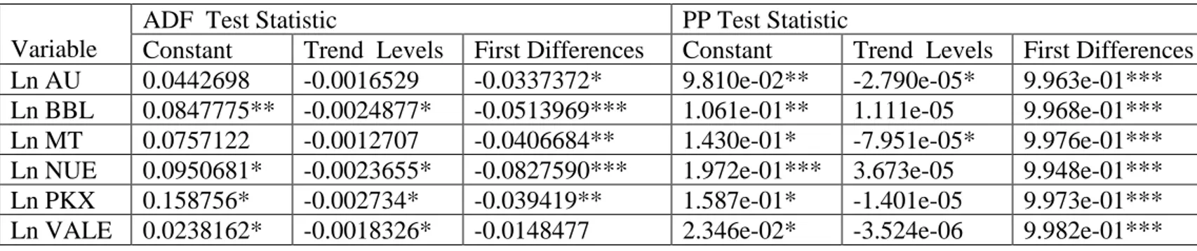
TABLE 4.1: FORMAL UNIT ROOT TEST. 39

TABLE 4.2: MODEL COMPARISON 46

TABLE 4.3: ERROR ANALYSIS 46

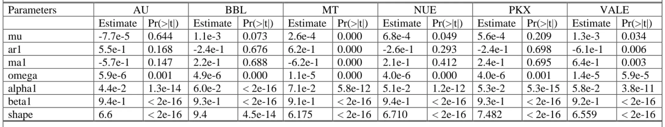
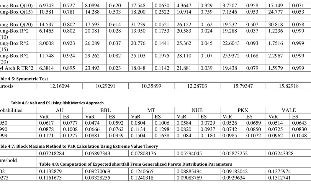
TABLE 4.4: STANDARDISED RESIDUALS TESTS 46

TABLE 4.5: SYMMETRIC TEST 47

TABLE 4.6: VAR AND ES USING RISK METRICS APPROACH 47

TABLE 4.7: BLOCK MAXIMA METHOD TO VAR CALCULATION USING EXTREME VALUE THEORY 47 TABLE 4.8: COMPUTATION OF EXPECTED SHORTFALL FROM GENERALIZED PARETO DISTRIBUTION

PARAMETERS 47

9

CHAPTER ONE

Introduction

Background

Investors' desire to make the most out of their investment can never be overestimated; this has led to investors or potential investors continually being on the lookout for better investment opportunities. This claim is empirically supported by scholars (Aharoni, 2015; Nisar, 2006; Haines Jr, Madill, & Riding, 2003 and Kelman, 2002), whose works claim that financial institutions, Due Diligence Private investors, etc. look for investment opportunities in and outside their geographical locations. The search is so intense that scholars like Zelitchenko (2009) recommend investors should go to the digital world and social network for these opportunities. While investors are seriously on the lookout, African countries' desperateness to attract foreign direct investment can never be overestimated (Osei-Fosu and Osei-Fosu, 2014). This statement is empirically supported by scholars (Constant & Tien, 2010; Thupa, 2019). In the same vein, there is a constant noise that Africa is the best place to invest if you want the most out of your investment (Arunga, 2008). It appears to be the newest destination for emerging market investors; the continent is expected to double the household consumption in the year more than 2030 (Signé, 2019). Not discounting all the above-stated investment opportunities Africa has to offer, the continent continues to struggle to attract investors (Pueyo, Spratt, Bawakyillenuo, Hoka & Osiolo, 2017; Enria, 2015). Whether local or foreign investors, they look elsewhere for investment opportunities while the continent of Africa is screaming with countless investment opportunities to offer (Troost, 2018; Boya, 2016; Ndulu, & Kiweu, 2015; Ndulu, 2010). The question as to why this continent is faced with this unfortunate treatment from all; leads to the age-old seemed-justified, but not an empirically verified argument of the continent being the riskiest place on earth to invest (Dmitriev, 2018; Mensah, 2016, March; Vasić, Bubaš, & Dario, 2016, January; Frobenius, n.d). Given the countless investment opportunities on this continent, how did the conclusion or claim regarding risk ever come about? People will quickly point to numerous armed conflicts on the continent (Berman, Couttenier, Rohner, & Thoenig, 2017; Williams, 2016), including insurgencies (Kleynhans, 2019; Bøås, 2019), militants (Awuni, 2013), insecurities (Chigbu, Paradza, & Mwesigye, 2019; Mawere, 2018), corruption (Fombad, 2020; Steytler, 2020; Adam, 2020), diseases (Iyioke, 2019). The list will go on and on to claim why the continent is the riskiest place on earth to invest (Becker & Payo, 2013). The question is, has there ever been any empirical evidence to support this age-old claim, other than what people have been made to believe will affect the value of their investment? Is there any empirical evidence of risk-comparative analysis for investment opportunities among continents in which Africa has been deemed the riskiest? Unfortunately, a search for answers to these questions and many more related questions has proved futile. I feel without legitimate and empirically verified answers to these, the continent will

10

continue to lose opportunities due to bad connotations. Good-willed individuals looking for the most out of their investments will settle for suboptimal since the optimal has been relegated from the equation. The quest to find answers to these concerns and other thought-provoking questions has led to this study's development. A study to offer legitimate answers to these questions has never been performed in Africa's demographic and psychographic representation or any part of the world. Current research has essential relevance and significance, if for no other reason than to start a conversation that could lead to the idea and/or manifestation to invest in the continent and fill this gap in the literature. This study plans to do so by examining time-series data of companies' adjusted stock prices from different continents listed on the stock market. Applying standard statistical procedures and Extreme Value Theory (EVT) to determine which continent’s company stock has the highest value at risk or conditional value at risk. The model will be evaluated by taking the data from Yahoo finance.

It is imperative to investigate, or help to estimate, the value of any would-be investment that will be at risk in purchasing stock from a country in Africa relative to other continents for the following reasons:

First, this study can contribute to already existing literature that seems to lack information about a comparative analysis of the value of an investment that is at risk, given the country or continent that the investment took place. It will also enrich and give the future literature a new dimension since it aims to tread on a never-used theoretical framework in this study of this phenomenon in a comparative manner.

Second, attitudes, behaviors, and investment decisions toward idiosyncratic countries or continents will be a critical factor influencing the development and management of “curse” resources (Paradox of Plenty) (Karl, 1997) in the future. “The resource curse, also known as the paradox of plenty, refers to the paradox that countries and regions with an abundance of natural resources, specifically point-source non-renewable resources like minerals and fuels, tend to have less economic growth and worse development outcomes than countries with fewer natural resources” Ross, (2015, p. 241). This is because if it is found that this whole categorization of the continent as the riskiest on earth is a mere myth, then probably investor could have the confidence and come in which could lead to a restructuring of resources which seems like a curse since at the moment it cannot be easily transformed to consumables.

Third, the world and most investors have been fearful of the amount of risk their investments could be subjected to if invested in Africa due to the unsubstantiated conventional belief and for that matter outsourced several companies to the east for cheaper labor which Africa could equally offer, this study could make it clear if Africa is one more option of where to outsource to if the idea is to access cheaper labor and also not expose their investment to the highest risk. If this opportunity is embraced, it will offer the world and humanity uniform distribution of consumable production centers around the globe, unlike the current situation where productions are situated in few areas hampering the world's efforts of stopping epidemics when they strike at production hops.

Again, this will help African countries who have suffered the wrath of this centuries-old unfair categorization once there is empirical liberation or confirmation. This is because investors who will be looking for only dividends out of their investment will not even bother to consider Africa as their investment location due to the riskiest tag attributed to the continent. For the same reason, it is equally suitable for the Good-willed individuals who are looking for the most out of their

11

investments since, unlike before, they will not have to settle for suboptimal with the possibility of optimal in the equation. For the same reason, it is good for the continent since it will only have to advertise about the opportunities it has to offer investors such as cheaper labor, available resource, etc. instead of spending time convincing investors about the continent been the riskiest or not. Finally, non-governmental organizations, inter-governmental organizations, individuals, etc. who care about the world's monetary system stability, poverty reduction, healthy life, etc. will benefit from this knowledge and aid in their resource allocations, campaigns, etc.

This study aims to use the extreme value theory, which seeks to assess, from a given-ordered sample of a given random variable, the probability of events that are more extreme than any previously observed. The theory is extensively used and a popular conceptual framework for the likelihood of events that are more extreme than any already found. It has been used in several studies and many areas, including structural engineering, finance, earth sciences, traffic prediction, public health, and geological engineering.

Problem Statement

The importance of uniform development across continents, regions, countries, cities, and towns can never be overemphasized (Cheema, 2005, December 08; Qureshi, 2005, December 08). The importance and demand for it have been made apparent to humanity and systems understanding in the 21st century because of the surge in economic mass migration across continents, countries, and cities (Ketola, 2017; Lundgren, 2009). In some cases, those who do not migrate and stay behind may devour the environment for their survival (Masron, & Subramaniam, 2019; Subramaniam, 2018), which contributes to the current climate situation humanity is facing (Kolo, 1991). Others see it as a grossly unfair distribution of wealth, and this may result in the selective use of violence against people or groups whom they feel are the beneficiaries (Wojciechowski, 2017; Tasgin, & Cam, 2016). Additionally, it becomes difficult or nearly impossible to stop a pandemic when it originates where production firms are situated (Didier, Huneeus, Larrain, & Schmukler, 2020). And, if these firms are the sole producers of a worldwide-needed product, it could conceivably put the whole of humanity at risk of extinction. All these happen in human history because jobs seem to have progressed in a few continents, countries, and cities, while majority of the world population is alienated from it (Ikhimwin & Obarisiagbon, 2020). These have taken place because of the lack of uniform or adequate investment in other parts of the world. The study feels some continents, countries, and cities are not getting sufficient investment to channel their growth and development because investors fear to lose their investments. The questions persist; how did investors decide to invest in some places, but not others? Are the information and resources on which the investors based their actions and inactions empirically justified and legitimate? The quest to answer these and many more mind-boggling questions have initiated this study. One of the best ways to find answers to some of these questions is to organize a comparative analysis of some financial derivatives from continent or countries that have won the benefit of the doubt of investors as compared to those that have not, and see if any of those entities are worthy of their situation discounting their growth gain as a result of the investment disparities. Studies tasked with responsibilities like these most often use extreme value theory to ascertain their outcomes.

12

Unfortunately, no research has ever taken into account the African experience, and it is the intent of this study to do so. Africa, as a continent, has its unique characteristics (Bloom et al., 1998), which makes it almost impossible to superimpose the outcomes of studies conducted in other geographical locations. Additionally, due to African history and nature (Beinart, 2013), the need to investigate factors that can impact opportunities for investment, such as investor confidence and centuries-old unfair categorization cannot be ignored. To refer to studies performed in other geographical locations in an attempt to understand Africa’s situation would be an injustice to Africa since the studies do not account for the aforementioned critical variables.

Since no study of this nature has ever been performed in Africa, it is the aim of this study to fill this gap in the literature. The study will examine which stock has the highest value at risk or conditional value at risk (expected shortfall) using standard statistical procedures and the extreme value theory.

Research Question

Through analysis, review, and presentation of data collected from prior studies and a secondary source, this study attempted to answer the question: Has Africa been fairly treated by investors by not offering it an adequate investment due to the fear of the value of their investment that could be at risk in comparison to investing it in another continent? To answer this question, the study investigated the comparative investment opportunities, the financial market, impact, and effect of lack of adequate investment in the continent; all of these have been considered in the literature review (LR) chapter. To explore factors predicted to influence the decision to invest in a place, the study employed a useful conceptual framework, the extreme value theory, and statistical procedures for identification and estimations; all have been reviewed in the literature review and methodology chapters, respectively. This investigation will lead to an inclusive and comprehensive understanding of investment opportunities and why investors should or should not invest in African countries since they have similar characteristics. This investigation will also enhance the comprehension of the influence of these factors and its generation of financial incentives.

Purpose

Many familiar scenes across the globe include inadequate infrastructural development for communities, cities, and countries; the rising unemployment figures; porous security; corruption; mass migration; etc. It is ubiquitous for people to conclude that most of the above-listed problems are a result of each other. But could there not be some other explanation for these problems. Many scholars, researchers, and laymen have suggested (Antwi‐Boateng, 2017; Isacson, Meyer, & Morales, 2014; Mawadza, 2008), or justified in some occasions that these factors affect chances of attracting investment. To date, no study has been conducted regarding a comparative analysis of risks relative to a value of an investment, nor has any study justified or scientifically proven how favorable or not favorable places relative to investment opportunities. It is the purpose of the study to fill this gap by assessing areas that have the highest value or conditional value at risk.

13

Specifically, the study aims at the following:

To seek a more precise understanding as to whether individual continents, countries, and cities deserve the faith embraced or embraced from investors.

To verify if individual continents, countries, and cities have been fairly or unfairly categorized, and how that has affected or is affecting their well-being.

Several studies (Bradshaw, 2007; Agrawal, & Redford, 2006) and reputable institutions (UN-ECA, 2012; UNDP, 2006) have drawn a link between poverty and lack of development or between the age of the continent, Africa, and its lack of progress. The study intends to ascertain as to whether the outcomes from the above-stated studies are the reasons for the lack of a fair proportion of the world investment to the continent.

Several studies and reputable institutions have established a link between poverty, development, unemployment, security, corruption, mass migration, etc. without looking at the possibility of lack of investment leading to all of these. The study aims to consider the direction of causality.

Significance

The contribution of this study to the body of research is multifaceted. It will be one of the first-ever studies to inquire about the rfirst-everse causality of lack of adequate investment opportunity leading to a lack of development, corruption, poverty, etc. Several studies have established unidirectional causality or link from insecurity, poverty, corruption to lack of investment opportunity. Could it not be that the reverse is the case? The study will be able to fill that gap in the literature by finding answers to that part of the relationship.

Studies have shown that the EVT model is useful and successful in examining value at risk and expected shortfall of stocks. It will be the first study to use EVT in a comparative analysis of stocks from different continents or countries.

Several studies and reputable institutions have established a link between poverty, development, unemployment, security, corruption, mass migration, etc. without looking at the possibility of lack of investment leading to all these. This study aims to provoke conversion about that direction of causality. The significance of the study lies in the provocation of argument about the course of the link, if there is one, and initiate a new conversation about the potential outcome and the need to reconsider our investment choices in the interest of humanity.

Rationale

Discussion about why there is inadequate investment in Africa relative to the rest of the world is hardly informed by rigorous evidence. Results from the present study should help to clarify this essential relationship, and thus contribute to our understanding as to why the issue exists and what can be done going forward to procure needed investments, and hopefully remedy the existing deficit created due to years of neglect.

The question as to whether the factors that influence decisions to invest in a place are similar across countries and continents is an important one. While previous research (Dmitriev, 2018; Mensah,

14

2016, March; Vasić, Bubaš, & Dario, 2016, January; Frobenius, n.d) regarding essential factors that influenced decisions to invest in non-Sub Saharan African (SSA) countries primarily suggests the security of that investment is paramount, it is not clear whether or not the evidence holds in all cases, when looking at current or past occurrences of places that have had investments. With the increasing emphasis on the importance of holistic economic growth in the world in general (Zeybek, 2018), it is essential that conclusions drawn regarding the factors used in the investment decision-making in all these other countries be validated in a context different than that used in SSA. Results from this study may contribute immensely to our knowledge in this regard.

The study should enhance the comprehension of interrelations of humans, their works, the biosphere, and the physical and other laws by which they are governed. This may, in effect, disprove the assumption that corruption, conflict, insecurity, etc. are repelling measures concerning attracting investment. These are the very reasons why these places should get investments so that people involved in these can get engaged in productive activities that the investments will create.

To meaningfully study the essential relationship between predictor variables and the decision to invest, the study must utilize the most rigorous method in establishing this relationship. This method should aid and guide policymakers in the region to make more informed decisions and formulate effective policies to attract foreign direct investment to the region. Hopefully, the study will bring broader understanding that the continent of Africa has been unfairly categorized over the years and justify that investments could help revert the current occurrences.

Definition of Terms

Generalized Autoregressive Conditional Heteroskedasticity (GARCH): statistical model used in analyzing time-series data where the variance error is believed to be serially autocorrelated. Autoregressive Conditional Heteroskedasticity (ARCH): statistical model for time series data that describes the variance of the current error term or innovation as a function of the actual sizes of the previous time periods’ error term and often the variance is related to the squares of the previous innovations.

Generalized pareto distribution: family of continuous probability distributions and it is often used to model the tails of another distribution. It is specified by three parameters that is the location, scale and shape.

(IGARCH)

Extreme value theorem: in calculus, it gives the existence of continuous function defined on close and bounded interval.

Student-t innovation (t-test): is any statistical hypothesis test in which the test statistic follows a student’s t- distribution under the null hypothesis.

15

Scope

This study tries to look at the empirical investigation of the difference in the value of investors’ investment that will be at risk, given the continent it is invested. Detailed theory and empirical review of variables will be taken into consideration. In order to predict the difference in the value of investors’ investment that will be at risk given the continent, it is invested the study will use most of the powerful and recent used economic techniques and identification strategies. The study will examine the stationarity or otherwise of the individual series by applying standard unit root test to each of the time series, giving that the series is stationary or corrected the study will train several Generalised Autoregressive Conditionally Heteroskedasticity (GARCH) models, because of its ability to model the conditional randomly varying volatility. The several GARCH models will be for a different order of the GARCH terms 2and the order of the ARCH terms 2and different distributions. The best GARCH model will be selected using the Akaike Information Criterion (AIC) and Bayesian Information Criterion (BIC). Data on the adjusted price of a systematic randomly selected stock from each continent will be taken from Yahoo finance, which will be used to test the validity of the model. Critical analysis of all the results that will be obtained from the said applied strategies will be presented. Finally, give useful recommendations that could go a long way to help in future research, investment market, investors, financial institutions, and policymakers.

Organization

The study is organized into six chapters. Chapter one is the introduction and gives a brief background to the study, statement of the problem, purpose, significance, rationale of the study, research question, definition of terms, the scope of the study, and the organization of the study. Chapter two discusses concepts and reviews relevant literature on the subject. Chapter three presents the methodology adopted for the study, including data and variable descriptions, and sources of data and statistical procedures for identification and estimations. Chapter four is devoted to the presentation and discussion of the empirical results. Chapter five concludes the study with summaries of significant findings and recommendations to set the agenda for future research in the same area. Chapter six presents the summary of reflection of objectives in the thesis.

16

CHAPTER TWO

Literature Review

This chapter places the study in context by reviewing the relevant literature and theories on investment, value-at-Risk, the various methodologies involved, and the assumptions underlining the measure. This chapter of the study seeks to find out what others have found and written about the subject under investigation. It focuses on the main issue under study, namely Value-at-Risk. It will proceed with brief definitions used to explain Value-at-Risk, then explores techniques in measuring value-at-Risk, and finally review other relevant theories for VaR estimation.

Investment

The term investment appears to be a common word whose understanding has been taken for granted. However, it is so robust that it needs to be explicitly explained on every occasion it is mentioned. The definition of investment is very relative and dependent on the context in which it is invoked. However, some ideas are constant in the description, regardless of the context: in every investment, it is understood to hold (through either purchase, embraced, etc.) some interest (which could be economic, psychological, emotional, physical, etc.) for future fulfillment (which could be economic gain, emotional gain, etc.). In terms of continents, countries, cities, etc. all the above multi-dimensional facets of investment hold, in the sense that others can invest for gain or the resources of the place can be invested in other areas for the present and or future fulfillments and so on.

For a better understanding of the terminology over the years, a lot of scholars, theorists, practitioners, etc. have tried to classify investment. Due to the reasons listed above, their efforts have never led to a uniformed consensus at which they are referring to the term determines it; thus, classification of the term is contingent upon individual definition and context. Based on the above, it is imperative to have an acute understanding of the concept of investment relative to the background, for fundamental or holistic understanding, there is the need for further research and comparisons, as this is where the field falls short.

Inadequate Investment in Africa

Even though it appears as if the continent of Africa has inadequate investment opportunities, how can one tell? One way to justify this is to examine what adequate investment leads to, compare it to the current African situation, and see if they align. Conversely, scrutinize the contemporary African situation, and see if it is reminiscent of adequate investment. The latter is what this section will take into consideration.

17

Several researchers and scholars (Rahman, 2020; Khan, Khan, Jiang, & Khan, 2020; Shaikh, Shaikh, & Talpur, 2019; Nanda, & Samanta, 2018; Gaal, & Afrah, 2017) have established that lack of infrastructure leads to a reduced standard of living, economic deficit, and poverty. Without any element of doubt, every individual will agree that all the effects of the lack of infrastructural development as listed above are the current definition of Africa (Dano, Balogun, Abubakar, & Aina, 2019; Chakamera, & Alagidede, 2018; Pieterse, Parnell, & Haysom, 2018). Knowing the devastating effect of lack of infrastructural development on a country and appreciating the idea that these are the typical scene in Africa, the next question is, what causes lack of infrastructure? Several scholars, institutions, and researchers (Yilema, & Gianoli, 2018; Sewell, & Desai, 2016; Mowarin, & Tonukari, 2010) will ascribe to several answers to this question, which include corruption, political influence, the inefficiency of the labor force, absence of incentives, poor accountability, and less political concern given to the sustainability of infrastructure service provision (Ngatia, Njoka, & Ndegwa, 2020; Kamoh, & Gyemang, 2018; Lawrence, 2016). All the above are legitimate causes of lack of infrastructure development, but what we lose sight of is they can also be classified as byproducts of lack of needed investment. For example, if the countries' institutions are strengthened through the right education, personnel, resources, legislation, etc., issues of corruption will be halted with these investments. If we agree on the fact that those mentioned above are the causes of lack of infrastructure development, and it is empirically established that they exist predominantly in African countries, and also agree that they are the result of inadequate investment, then we can empirically and existentially determine by transitivity that African countries are suffering from lack of needed investment.

Reasons for Choosing a Place for Investment

The fundamental reason why everyone invests is to ensure their present and future financial security that they need for the acquisition of other services and fulfillment. The fact that the idea to invest incorporates present and future needs or, to a more considerable extent, wants to make the decision very crucial. Due to the importance that surrounds the reason why in the first place, people invest makes understanding the factors that influence their decision of where and what to invest more vital. This section is seeking to understand the factors that influence investors' choice of where and what to invest.

According to several scholars (Joshi, 2013; Horner & Aoyama, 2009), the cardinal factors that influence almost every investors' decision of what and where to invest are risk and reward, and those two are highly intertwined (Bruce, Potter, & Roy, 1995). Thanks to a lot of body of knowledge, a lot of work has been done, and markets, continents, countries, cities, towns, places, etc. have been classified in terms of how risky it is to invest in them (Butt, 2015; Rufino, Cariňo, Ong, & Orbeta, 2013). Investment experts always advocate investors should make sure their places of investment match the same level of risk they are willing or capable of taking on their portfolio (Pula, Berisha, & Ahmeti, 2012; Schooley, & Worden, 2003). Again, great work has been done on how to foretell a place's level of risk and how to align them with an individual's levels of risk (Leiss, & Nax, 2016, June; Terzić, & Milojević, 2013, June). In terms of assessing individuals’ places level of risk is by using the accepted norm, which is classifying places into developed and

18

emerging markets (Worthington, & Higgs, 2004). Within these two big umbrellas, other factors such as security, economy, sector, market collapses, political upheaval, etc. should be considered to perceive the risk level. Once the place to invest has been identified, further investigation is needed based on other investment characteristics (demand, supply, security, stability, history, etc.) to determine the sector and down to the very organization, the investor wants to invest in (Leiss, & Nax, 2016; Butt, 2015).

It must be acknowledged that investors can make choices of places, sectors, and the exact organizations they want to invest based on the risk, as discussed above, and their associated rewards. This idea welcomes the concept of investors' risk tolerance level, and most of the time, the higher the risk the investment imposes the higher the returns of reward it offers and vice versa (Zhang, Huang, & Zhang, 2015; Pula, Berisha, & Ahmeti, 2012). Hence having all these at investors' disposal, the investors need to evaluate their willingness to lose their investment should all things go wrong in exchange for its equivalent rewards should every go according to plan (Pula, Berisha, & Ahmeti, 2012). This is the trickiest part of investment decisions, but most of the time, investors are guided through these by professionals. It must be noted that all the above is the conventional investment search by investors. Still, there are situations where others invest in a place or organization for other uncountable reasons such as nonprofit purpose, emotional attachment, control, etc. (Dreyer, 2014; Micheels, Katchova, & Barry, 2004).

Types of Risk measure

The study aims to review and use the two most used risk measures, which are value at risk (VaR) and conditional value at risk, also knowns as expected shortfall (ES). In both risk measures, the study will also review the types of ways they can be estimated.

Value-at-Risk (VaR)

VaR is a measure of the risk of investments. It estimates how much a set of investments might lose, given normal market conditions, in a set period such as a day. In its most general form, the VaR measures the potential loss in value of a risky asset or portfolio over a defined period for a given confidence interval. VaR measures the maximum expected loss over a given period at a given confidence level that may arise from uncertain market factors.

In its adapted form, the measure is sometimes defined more narrowly as the possible loss in value from “normal market risk” as opposed to all risk, requiring that we draw distinctions between normal and abnormal risk as well as between market and non-market risk.

While Value-at-Risk can be used by any entity to measure its risk exposure, it is used most often by commercial and investment banks to capture the potential loss in value of their traded portfolios from adverse market movements over a specified period. The major challenge in implementing VaR analysis is the specification of the probability distribution of extreme returns used in the calculation of the VaR estimate.

19

While the term “Value at Risk” was not widely used before the mid-1990s, the origins of the measure lie further back in time. The mathematics that underlies VaR was developed mainly in the context of portfolio theory by Harry Markowitz and others. However, their efforts were directed towards a different end – devising optimal portfolios for equity investors. In particular, the focus on market risks and the effects of the co-movements in these risks are central to how VaR is computed.

The impetus for the use of VaR measures, though, came from the crises that beset financial service firms over time and the regulatory responses to these crises. The first regulatory capital requirements for banks were enacted in the aftermath of the Great Depression and the bank failures of the era when the Securities Exchange Act established the Securities Exchange Commission (SEC) and required banks to keep their borrowings below 2000% of their equity capital. In the decades after that, banks devised risk measures and control devices to ensure that they met these capital requirements. With the increased risk created by the advent of derivative markets and floating exchange rates in the early 1970s, capital requirements were refined and expanded in the SEC’s Uniform Net Capital Rule (UNCR) that was promulgated in 1975, which categorized the financial assets that banks held into twelve classes, based upon risk, and required different capital requirements for each, ranging from 0% for short term treasuries to 30% for equities. Banks were required to report on their capital calculations in quarterly statements that were titled Financial and Operational Combined Uniform Single (FOCUS) reports.

The first regulatory measures that evoke Value at Risk, though, were initiated in 1980, when the SEC tied the capital requirements of financial service firms to the losses that would be incurred, with 95% confidence over a thirty-day interval, in different security classes; historical returns were used to compute these potential losses. Although the measures were described as haircuts and not as Value or Capital at Risk, it was clear that SEC required financial service firms to embark on the process of estimating one-month 95% VaRs and hold enough capital to cover the potential losses. At about the same time, the trading portfolios of investment and commercial banks were becoming more significant and more volatile, creating a need for more sophisticated and timely risk control measures. Ken Garbade at Banker’s Trust, in internal documents, presented advanced measures of Value at Risk in 1986 for the firm’s fixed income portfolios, based upon the covariance in yields on bonds of different maturities. By the early 1990s, many financial service firms had developed rudimentary measures of Value at Risk, with wide variations on how it was measured. In the aftermath of numerous disastrous losses associated with the use of derivatives and leverage between 1993 and 1995, culminating with the failure of Barings, the British investment bank, as a result of unauthorized trading in Nikkei futures and options by Nick Leeson, a young trader in Singapore, firms were ready for more comprehensive risk measures. In 1995, J.P. Morgan provided public access to data on the variances of and covariances across various security and asset classes, that it had used internally for almost a decade to manage risk, and allowed software makers to develop software to measure risk. It titled the service “RiskMetrics” and used the term Value at Risk to describe the risk measure that emerged from the data. The proposal found a ready audience with commercial and investment banks, and the regulatory authorities overseeing them, who warmed to its intuitive appeal. In the last decade, VaR has become the established measure of risk exposure in financial service firms and has even begun to find acceptance in non-financial service firms.

20

Measuring Value-at-Risk

Three basic approaches are used to compute Value-at-Risk, though there are numerous variations within each strategy. The measure can be calculated or estimated with the use of the Variance-Covariance method (VCM), Monte Carlo simulation (MS), and historical simulation (HS), all showing specific advantages and disadvantages. Jorion (1997) and Dowd (1998) present a detailed treatment of these methods. Manfredo and Leuthold (1999) discuss the pros and cons of these estimation procedures. In this section, we describe and compare the approaches.

Variance-Covariance Method (VCM)

The variance-covariance method (also called the parametric approach or delta-normal method) determines VaR directly as a function of the volatility of the portfolio return. The VCM is the analytical approach used for calculating VaR, and it is the most straightforward formula used for the calculation since VaR gives a measurement of the maximum loss that financial firms are likely associated with, within a specific period. During the process of the forecast, the variance-covariance observes the movement of the instrument over time and uses the probability theory to evaluate the associated maximum loss.

An apparent advantage of the VCM is its ease of computation. If the normality assumption holds, VaR figures can be simply translated across different holding periods and confidence levels. Moreover, time-varying volatility measures can be incorporated, and what-if –analyses are easy to conduct. On the other hand, the normality assumption is frequently criticized. There is empirical evidence that return distributions are fat-tailed, and in that case, the VCM will underestimate the VaR for high confidence levels. Further problems occur if the portfolio return depends in a nonlinear way on the underlying risk factors, which is typically the case when options are included in the portfolio.

Historical Simulation (HS)

HS resembles the Monte Carlo simulation regarding the iteration steps. The difference is that the value changes of the portfolio are not simulated employing a random number generator but directly calculated from observed historical data. That means VaR estimates are derived from the empirical profit-and-loss distribution. Hence, no explicit assumption about the return distribution is required. However, this procedure implicitly assumes a constant (stable) distribution of the market factors. Among all the approaches for estimating VaR, historical simulation is the simplest way of estimating VaR when it comes to many portfolios. With this approach, a hypothetical time series of returns on the portfolio is created by running the portfolio through the actual historical data. Then the changes in each period are computed. Also, since the portfolio over time yields all the information needed to calculate the VaR, there is no need to use the data to estimate the variance and covariance.

21

Monte-Carlo Simulation

With this method, the entire distribution of the portfolio's value change is generated, and VaR is measured as an appropriate quantile from the relative frequency distribution. Among the two approaches mentioned above, Monte-Carlo simulation is the most complicated one. It has several advantages and disadvantages to deterministic analysis. Some of the benefits are:

The probabilistic result shows not only what happens but also how likely each outcome will be. The graphical results: since the Monte-Carlo simulation generates a lot of data, it is easy to create graphs of different issues and their chance of occurrence, and it is vital for communicating findings to other stakeholders.

Scenario analysis: in deterministic models, it is not straightforward to model different inputs to precisely see which inputs had values together when specific outcomes occur; it is invaluable for further analysis. Sensitivity analysis: with just a few cases, the deterministic analysis makes it difficult to see which variables impact the other. In this simulation, it is easy to see which inputs had the most significant effect on the bottom-line results.

Extreme Value Theory

In the review of VaR, some pitfalls of traditional methods of VaR estimation became apparent, in particular, if the prediction of infrequent events is desired and leptokurtic distributions are involved. Now we turn to the Extreme Value Theory (EVT) to improve the estimation of extreme quantiles. EVT provides statistical tools to estimate the tails of probability distributions. Much more comprehensive treatment can be found in Embrechts, Klüppelberg, and Mikosch (1997). Embrechts, Klüppelberg, and Mikosch (1997, p. 364) cite that the main objective of the EVT is to make inferences about sample extrema (maxima or minima). The extreme value theorem focuses only on the tails of distribution-extreme rare events, especially useful for calculation of high-confidence level VaR, which reflects the sporadic losses in the distribution tail. Key inputs for the EVT model are the tail index and the inverse of the tail index (shape) parameters. Usually, for risk calculations, one of the three types of tails are considered: finite endpoint, normal, and fat-tailed (Student-t).

22 Figure 2.1: Graph of Extreme Value Distributions (Source: Jon Danielson (2017, p. 11))

From the above graph, the black line indicates the Weibull distribution, which has a finite endpoint. The red line also shows the Gumbel distribution, which has a normal tail, and one can see that the Frechet tail is thicker done that of the Gumbel. Lastly is the blue line, which indicates the Frechet tail distribution, which also has a fat tail. We know that in most applications in finance, the returns are fat-tailed, and hence we limit our attention to the Frechet case.

If we assume that, the return r , where _t t=1, 2, 3,...,n are serially independent of periods and has a common cumulative distribution function F x where x is the set of all real numbers, then the

( )

range of the return r is given as _t

 

l u which defines the extreme values of the function, where l , stand for the infinitesimal minimum and u stands for the infinitesimal maximum of the function. For a log return, we will have l = − and u =  . The cumulative density function (CDF) of r is ₁ denoted as F_n,1

( )

x is given as

( )









,1 Pr 1 1 Pr 1 n F x = r x = − r  x 2.1 = −1 Pr



r₁ x r, ₂ ,...,r_n  n



(

)

1 1 Pr n j j r x =

= −



 under independent assumption

(

)

1 1 1 Pr n j j r x =   = −



_ −  _

( )

1 1 1 n n j F x = = −



_ − _ = − −1 _1 F x

( )

_ n.

23

The above equation shows that as n increases to infinity, F_n,1

( )

x declines that are F_n,1

( )

x → if 0 1

x  and F_n,1

( )

x → if 1 x  as n approaches infinity. Also, the declination of the CDF has no 1 practical value. Under the independent assumption, the limiting distribution of the normalized minimum r_{( )1}* is given as:

 





( )

1 * 1 exp 1 , 0 1 exp exp , 0 k kx k F x x k  ₋ _{− +}  _  _ _ =   − _− _ =  2.2 For x 1 k  − if k  and 0 x 1 k  − if k  0 Where

The subscript * signifies the minimum k and k is referred to as the shape parameter which controls the tail behavior of the limiting distribution.

1 k

 = − is called the tail index of the distribution.

Type I: k = , is called the Gumbel Family and its CDF is given as, 0

 

 

* 1 exp exp

F x = − _− x _,

Where −   x .

Type II: k  , is called the Frechet family and its CDF is given as, 0

 





1 * 1 1 exp 1 , 1, k kx x F x k otherwise  ₋ _{− +}  _{ −}  _{ } =_{  }  2.3

Type III: k  , is called the Weibull family and its CDF is given as 0

 





1 * 1 1 exp 1 , 0, k kx x F x k otherwise  ₋ _{− +}  _{ −}  _{ } =_{  }  2.4

Risk managers are most interested in the Frechet family, which involves stable and student-t distribution. The probability density function (pdf) of the generalized extreme value theory can be obtained by differentiating equation 2.2 which is given as,

 









 

1 1 1 * 1 exp 1 , 0 exp exp , 0 k k kx kx k F x x x k −  ₊ _{− +}  _  _ _ =   _{ −  =}    2.5

24

Extreme Value Estimations

There are two types of extreme value estimations, which are the block maxima (minima) and the peak over the threshold.

Parameter Estimation Using Block Maxima Method

For a given sample, we have one maximum, which means estimation for the three parameters

(

  , _n, _n

)

will be very difficult since it has only one extreme observation. To rectify this problem, one needs alternative ways to solve it. The alternative way to do this is to divide the sample into subsample and then apply the extreme value theory (EVT) to the subsamples.

Suppose that we have T returns that are

 

1

T j _j

r

= , then we divide the sample into g non-overlapping

subsamples each with n-observation that is if we assume simplicity that T =ng. From a practical viewpoint, there are 21trading days in a month, which implies that the daily return n =21.

Let r be the maximum of the n i,

th

i subsample that is the largest return, where the subscript n represents the size of the subsamples. Therefore, the new variable r from each of the subsamples n i,

is given as: , , n i n n i n x r   −

= , where x_{n i,} =



x_{( )i j n j− +}



for 1 j n , and i=1, 2, 3,...,q. 2.6 The data we get from the collection of the subsample max



r_{( )i j n j− +}



are used to estimate the unknown parameters of the extreme value theory. Also, one can use the maximum likelihood method or the regression method to determine the unknown parameters



  , _n, _n



when the probability density function of r is known since the sub-periods maxima n i, max



x( )i j n j− +



follows

a generalized extreme value (GEV) distribution.

Extreme Value Theory for Peak Over Threshold Method

As we described above, the block maxima method to VaR calculation using extreme value theory has its defaults, that is, the sub-period length n is not clearly defined.

The method is also unconditional and does not take into consideration the effects of other explanatory variables.

To improve the defaults, we introduce a new approach which is called the Peak Over Threshold (POT) method, which focuses mainly on the exceedances of the measurement over some high specific threshold. Also, the peak over threshold uses information more efficiently by considering more than one sample.

25

The peak over threshold method considers the conditional distribution of x= − given the r_t  information that  for a long position and the occurrence of the event r_t  which follows a r_t Poisson distribution.

Now we consider the conditional distribution of r= + which is the basic theory of the peak x  over threshold method given that r , since that process of the peak over threshold does not  need the choice of sub-period length n hence no need to use the subscript of the parameter. We now define the probability of the conditional distribution of r + given rx   as 

(

)

Pr

(

₍

₎

)

Pr

(

₍

)

Pr

(

₎

)

Pr | Pr 1 Pr r x r x r r x r r r           +  + −   +  = =  −  2.7

Now let denote the cumulative density function as F which implies that _*

(

)

*

(

)

_{( )}

*

( )

* Pr | 1 F x F r x r F      + −  +  = − and defined F as _*

( )

(

)

1 * 1 exp , 0 exp exp , 0 n k n n n n n n n k r k F r r k       _{ − − }   _{− }  _   _{ }   _{ }   _{  − }  _{−   =}  _{  }  2.8

Then in the case of k  we have, 0

(

)

(

)

(

)

(

)

1 1 1 1 1 exp exp Pr | 1 1 exp k k k k x k r x r k                − + − − −     _{− } ₋ _{− }   _{ }   _{ }           +  =  _{ − − }    − _{−  }      

(

)

₍

₎

1 Pr | 1 1 k kx r x r k         +   − −_{ } − −   2.9 Where x  and 0 1 k

(

 

)

0  − − 

26

(

)

exp exp exp exp

Pr | 1 exp exp x r x r            ₋  + − ₋ ₋  −       _{ } _{  }_    +  =   −  − _− _{ }    

(

)

Pr r x  1 exp x     +  − _− _   2.10

Expected Shortfall

Many authors have criticized the adequacy of VaR as a measure of risk. Artzner et al. (1997, 1999) propose, as an alternative measure of risk, the Expected Shortfall, which measures the expected value of portfolio returns given that some threshold (usually the Value at Risk) has been exceeded. The expected shortfall is a risk measure that is a measure used to determine the amount of asset or set of assets to be kept in reserve. It is also a tool that is used in financial risk measurement to evaluate the amount of market risk and credit risk of a portfolio. The expected shortfall is also known as the expected tail loss (ETL), conditional value at risk (cVaR), and the average value at risk (AVaR). For expected shortfall with confidence level  we can see that when the average loss exceeds the value at risk at the same confidence level  , then we can write expected shortfall mathematically as

 

1 1

 

1 t ES L VaR L dt   = −



2.11

For a loss L, the continuous loss distribution from the above equation can be rewritten as

 

|

 

ES_ L =E L L_ VaR L _ 2.12

where the expected value is taken throughout the equation and integrated. The diagram below shows the expected shortfall in contrast to VaR.

27 Figure 2.2: Graph of Expected shortfall in contrast to VaR (Source: Portfolio Mason (2018))

The Expected shortfall, in contrast to VaR, gives information about the losses that occur when the confidence level is exceeded and thus can potentially evaluate the extreme losses in the distribution tail.

Modeling the Return Distribution

If a parametric approach to VaR estimation is utilized, the question arises which distribution function fits best to the observed changes of the market factors? As mentioned above, it is widely recognized in the literature that fat tails characterize empirical return distributions of financial assets. Concerning modeling the underlying stochastic process, two consequences can be deduced (Jorion, 1997, p. 166 f.): either one uses a leptokurtic distribution, e.g., at -distribution or one resorts to a model with stochastic volatility and both approaches can be combined. The observation of volatility clusters in high frequency (i.e., daily) data favors the use of models with stochastic volatilities. For example, the changing of phases of relatively small and relatively high fluctuations of returns can be captured with GARCH models.

ARCH Model

The ARCH model was the model proposed by Engle (1982), which was invented purposely to provide a systematic framework for volatility models. To be more precise, the general ARCH (m) model assumes that,

28 t t t a =  , 2 2 2 0 1 1 ... t at m t ma  = + ₋ + + ₋ . 2.13 so for an ARCH (1) model, we will have

1 1 1 a =  , 2 2 1 0 1 0a  = + Where t

a is a function of the stochastic error term,

0 0

  and _i  for 0 i  0

t

 is the error term which is a sequence of independent and identically distributed (iid) random variables with mean 0 and variance 1.

For simplicity and easy understanding of the properties under the ARCH Model, the following Stationarity and Normality assumptions will later be used for our equations.

1) It is assumed under the stationarity assumption,



1|



t t t

a =E a₊ I

2) It is assumed under the stationarity assumption,

 

2

var

t t

E a  =_{ } a

3) It is assumed under stationarity assumption,

 

2 2

1 var 1 var

t t t

E a_{ −} _= _a₋ _= a

4) The normality assumption states that the expectation of the error term is zero. That is

 

_t 0

E  =

The mathematics below will explain the properties of the ARCH model, and we will begin with the first property, which states that the unconditional mean of the shock

( )

a remains zero. From _t the first assumption above and knowing that

at = t t

Then we have,



| 1



t t t t t

a =  =E a I₋

where I_t−1 denotes the information set, which is the set containing all the past returns up to and including time t − . 1

29

 

t



t 1| t





t t



E a =E a₊ I =E  

since _t is entirely determined by the filtration at t+1 from equation 2.13, hence we can only take expectation on the error term, and this gives,

E a

 

_t =_tE

 

_t

From the normality assumption, the expectation of the error term is zero. This implies that,

0 0 t   = Therefore

 

t



t 1| t



t

 

t 0 E a =E a₊ I = E  =

Secondly, the unconditional variance of the shock

( )

a can be seen as _t

2 2

1|

t t t

E a _{ }=E a_{ +} I _

From the second assumption in the stationarity assumption above,

 

2

var

t t

E a  =_{ } a This implies that,

 

2 2 1 var a_t =E a_{ } _t =E a_ _t+ |I_t_ but 2 2 0 1 1 t t a = + a₊

and substituting this into the above equation gives

 

2 0 1 1 var a_t =E_ + a_t+ _

 

2 0 1 1 var a_t = + E a_{ t+} _

From the third assumption above,

 

2 2

1 var 1 var

t t t

E a_{ +} _= _a₊ _= a

and substituting it into the above equation gives,

 

0 1

 

var a_t = + var a_t

 

1

 

0 var a_t − var a_t =

 

1



0 var a_t 1− =

 

0 1 var 1 t a   = − . 2.14

the variance of a must be positive and this means that _t ₁ should be between 0 and 1 that is

1

0  . 1

Lastly, in some applications, one might need a higher-order moment of a . In such cases, _t ₁ must satisfy some additional constraints. This means that we need the fourth moment of a to be finite. _t

30

From equation 2.13 and the normality assumption of _t, the general equation for the ARCH model was given as,

t t t

a =  , _t2 = ₀+ _ta_t2₋₁+ +... _{m t m}a2₋ .

To understand the ARCH model, one needs to carefully study the law of iterated expectation on the conditional distribution (LIE).1 This is because the ARCH model extensively use the law of iterated expectation in its model especially when it comes to its fourth moment.

To begin with, 4 4 1 1| t t t E a_{ +} _=E a_{ +} I _ By definition, 4 4 4 1 1 1 t t t a₊ = _{+ +}

Substituting the definition of a_t4₊₁ into the equation gives,

4 4 4

1 1 1|

t t t t

E a_{ + }=E_ _{+ +} I _

since _t4₊₁ is entirely determine by the filtration to t + , hence we only take expectation on the 1 error term, and this gives,

4 4 4 1 1 1| t t t t E a_ _{+ }=₊E_₊ I _ 2 4 2 4 1 1 1| t t t t E a_ _{+  } = ₊ _ E_ ₊ I _ Substituting 2 2 1 0 1 t at

₊ = + into the equation gives,

2

4 2 4

1 0 1 1|

t t t t

E a_ _{+  } =  + a _ E_₊ I _

In this case, the error term is a standard normal variable, and we need to take the fourth moment of it. For the calculation of the error term, we will need the formula below

In this case, X is our error term

 

_t+1 from the equation of the LIE and the error term is an independent and identically distributed (iid) with mean 0 and variance 1 that is  = , P is 4, 1





4 4 1 4 1 !! t E_₊  =_  −





4 4 1 1 4 1 !! t E_₊  =_ − 4 1 3!! t E_₊  =_

The double factorial of 3 is 3

Therefore, the fourth moment of the error term is 3 and substituting this back into the previous equation gives,

1 _{The law of iterated expectation is defined as the unconditional expectation of a random variable say Y is equal to} the expected of the expected value of Y given some other variable X. which is mathematically written as

 



|

