Abstract—This paper explores the possibility of using the Hierarchical Temporal Memory (HTM) machine learning technology to create a profitable software agent for trading financial markets. Technical indicators, derived from intraday tick data for the E-mini S&P 500 futures market (ES), were used as features vectors to the HTM models. All models were configured as binary classifiers, using a simple buy-and-hold trading strategy, and followed a supervised training scheme. The data set was divided into a training set, a validation set and three test sets; bearish, bullish and horizontal. The best performing model on the validation set was tested on the three test sets. Artificial Neural Networks (ANNs) were subjected to the same data sets in order to benchmark HTM performance. The results suggest that the HTM technology can be used together with a feature vector of technical indicators to create a profitable trading algorithm for financial markets. Results also suggest that HTM performance is, at the very least, comparable to commonly applied neural network models.
I. INTRODUCTION
URING the last two decades there has been a radical
shift in the way financial markets are traded. Over time, most markets have abandoned the pit-traded, open-outcry system for the benefits and convenience of the electronic exchanges. As computers became cheaper and more powerful, many human traders were replaced by highly efficient, autonomous software agents, able to process financial information at tremendous speeds, effortlessly outperforming their human counterparts. This was enabled by advances in the field of artificial intelligence and machine learning coupled with advances in the field of financial market analysis and forecasting. The proven track record of using software agents in securing substantial profits for financial institutions and independent traders has fueled the research of various approaches of implementing them. This paper incorporates technical indicators, derived from the E-mini S&P 500 future market, with a simple buy-and-hold trading strategy to evaluate the predictive capabilities of the Hierarchical Temporal Memory (HTM) machine learning technology.
Chapter II gives background information on technical analysis, predictive modeling and the HTM technology, followed by a review of related work in chapter III. Chapter IV details the methodology used to train, validate and test HTM classifiers. The results are presented in chapter V. Chapter VI contains conclusions and suggested future work.
School of Business and IT, University of Borås, Sweden (e-mail: {patrick.gabrielsson, rikard.konig, ulf.johansson}@hb.se).
II. BACKGROUND A. Technical Analysis
The efficient market hypothesis was developed by Eugene Fama during his PhD thesis [1], which was later refined by himself and resulted in the release of his paper entitled
“Efficient Capital Markets: A Review of Theory and Empirical Work” [2]. In his 1970 paper, Eugene Fama
proposed three types of market efficiency; weak form, semi-strong form and semi-strong form. The three different forms describe what information is factored into prices.
In strong form market efficiency, all information, public and private, is included in prices. Prices also instantly adjust to reflect new public and private information. Strong form market efficiency states that no one can earn excessive returns in the long run based on fundamental information. Technical analysis, which is based on strong form market efficiency, is the forecasting of future price movements based on an examination of past movements. To aid in the process, technical charts and technical indicators are used to discover price trends and to time market entry and exit. Technical analysis has its roots in Dow Theory, developed by Charles Dow in the late 19th century and later refined
and published by William Hamilton in the first edition (1922) of his book “The Stock Market Barometer” [3]. Robert Rhea developed the theory even further in “The Dow
Theory” [4], first published in 1932. Initially, Dow Theory
was applied to two stock market averages; the Dow Jones Industrial Average (DJIA) and the Dow Jones Rails Average, which is now the Dow Jones Transportation Average (DJTA).
Modern day technical analysis [5] is based on the tenets from Dow Theory; prices discount everything, price movements are not totally random and the only thing that matters is what the current price levels are. The reason why the prices are at their current levels is not important. The basic methodology used in technical analysis starts with an identification of the overall trend by using moving averages, peak/trough analysis and support and resistance lines. Following this, technical indicators are used to measure the momentum of the trend, buying/selling pressure and the relative strength (performance) of a security. In the final step, the strength and maturity of the current trend, the reward-to-risk ratio of a new position and potential entry levels for new long positions are determined.
Hierarchical Temporal Memory-Based Algorithmic Trading of
Financial Markets
Patrick Gabrielsson, Rikard König and Ulf Johansson
B. Predictive Modeling
A common way of modeling financial time series is by using predictive modeling techniques [6]. The time series, consisting of intra-day sales data, is usually aggregated into bars of intraday-, daily-, weekly-, monthly- or yearly data. From the aggregated data, features (attributes) are created that better describe the data, e.g. technical indicators. The purpose of predictive modeling is to produce models capable of predicting the value of one attribute, the dependent variable, based on the values of the other attributes, the independent variables. If the dependent variable is continuous, the modeling task is categorized as regression. Conversely, if the dependent variable is discrete, the modeling task is categorized as classification.
Classification is the task of classifying objects into one of several predefined classes by finding a classification model capable of predicting the value of the dependent variable (class labels) using the independent variables. The classifier learns a target function that maps each set of independent variables to one of the predefined class labels. In effect, the classifier finds a decision boundary between the classes. For 2 independent variables this is a line in 2-dimensional space. For N independent variables, the decision boundary is a hyper plane in N-dimensional space.
A classifier operates in at least two modes; induction (learning mode) and deduction (inference mode). Each classification technique employs its unique learning algorithm to find a model that best fits the relationship between the independent attribute set and the class label (dependent attribute) of the data.
A general approach to solving a classification problem starts by splitting the data set into a training set and a test set. The training set, in which the class labels are known to the classifier, is then used to train the classifier, yielding a classification model. The model is subsequently applied to the test set, in which the class labels are unknown to the classifier. The performance of the classifier is then calculated using a performance metric which is based on the number of correctly, or incorrectly, classified records. One important property of a classification model is how well it generalizes to unseen data, i.e. how well it predicts class labels of previously unseen records. It is important that a model not only have a low training error (training set), but also a low generalization error (estimated error rate on novel data). A model that fits the training set too well will have a much higher generalization error compared to its training error, a situation commonly known as over-fitting.
There are multiple techniques available to estimate the generalization error. One such technique uses a validation set, in which the data set is divided into a training set, a validation set and a test set. The training set is used to train the models and calculate training errors, whereas the validation set is used to calculate expected generalization errors. The best model is then tested on the test set.
C. Hierarchical Temporal Memory
Hierarchical Temporal Memory (HTM) is a machine learning technology based on memory-prediction theory of brain function described by Jeff Hawkins in his book On
Intelligence [7]. HTMs discover and infer the high-level
causes of observed input patterns and sequences from their environment.
HTMs are modeled after the structure and behavior of the mammalian neocortex, the part of the cerebral cortex involved in higher-level functions. Just as the neocortex is organized into layers of neurons, HTMs are organized into tree-shaped hierarchies of nodes (a hierarchical Bayesian network), where each node implements a common learning algorithm [8].
The input to any node is a temporal sequence of patterns. Bottom layer nodes sample simple quantities from the environment and learn how to assign meaning to them in the form of beliefs. A belief is a real-valued number describing the probability that a certain cause (or object) in the environment is currently being sensed by the node. As the information ascends the tree-shaped hierarchy of nodes, it incorporates beliefs covering a larger spatial area over a longer temporal period. Therefore, higher-level nodes learn more sophisticated causes in the environment [9].
In natural language, for example, simple quantities are represented as single letters, where the higher-level spatiotemporal arrangement of letters forms words, and even more sophisticated patterns involving the spatiotemporal arrangement of words constitute the grammar of the language assembling complete and proper sentences.
Frequently occurring sequences of patterns are grouped together to form temporal groups, where patterns in the same group are likely to follow each other in time. This contraption, together with probabilistic and hierarchical processing of information, gives HTMs the ability to predict what future patterns are most likely to follow currently sensed input patterns. This is accomplished through a top-down procedure, in which higher-level nodes propagate their beliefs to lower-level nodes in order to update their belief states, i.e. conditional probabilities [10, 11].
HTMs use Belief Propagation (BP) to disambiguate contradicting information and create mutually consistent beliefs across all nodes in the hierarchy [12]. This makes HTMs resilient to noise and missing data, and provides for good generalization behavior.
With support of all the favorable properties mentioned above, the HTM technology constitutes an ideal candidate for predictive modeling of financial time series, where future price levels can be estimated from current input with the aid of learned sequences of historical patterns.
In 2005 Jeff Hawkins co-founded the company Numenta Inc, where the HTM technology is being developed.
Numenta provide a free legacy version of their development platform, NuPIC, for research purposes. NuPIC version 1.7.1 [13] was used to create all models in this case study.
III. RELATED WORK
Following the publication of Hawkins' memory-prediction theory of brain function [7], supported by Mountcastle's unit model of computational processes across the neocortex [14], George and Hawkins implemented an initial mathematical model of the Hierarchical Temporal Memory (HTM) concept and applied it to a simple pattern recognition problem as a successful proof of concept [15]. This partial HTM implementation was based on a hierarchical Bayesian network, modeling invariant pattern recognition behavior in the visual cortex.
Based on this previous work, an independent implementation of George's and Hawkins' hierarchical Bayesian network was created in [16], in which its performance was compared to a back propagation neural network applied to a character recognition problem. The results showed that a simple implementation of Hawkins' model yielded higher pattern recognition rates than a standard neural network implementation, hence confirming the potential for the HTM concept.
The HTM model was used in three other character recognition experiments [17-19]. In [18], the HTM technology was benchmarked against a support vector machine (SVM). The most interesting part of this study was the fact that the HTM's performance was similar to that of the SVM, even though the rigorous preprocessing of the raw data was omitted for the HTM. A method for optimizing the HTM parameter set for single-layer HTMs with regards to hand-written digit recognition was derived in [19], and in [17] a novel study was conducted, in which the HTM technology was employed to a spoken digit recognition problem with promising results.
The HTM model was modified in [20] to create a Hierarchical Sequential Memory for Music (HSMM). This study is interesting since it investigates a novel application for HTM-based technologies, in which the order and duration of temporal sequences of patterns are a fundamental part of the domain. A similar approach was adopted in [21, 22] where the topmost node in a HTM network was modified to store ordered sequences of temporal patterns for sign language recognition.
Few studies have been carried out with regards to the HTM technology applied to algorithmic trading. Although, in 2011 Fredrik Åslin conducted an initial evaluation [23], in which he developed a simple method for training HTM models for predictive modeling of financial time series. His experiments yielded a handful of HTM models that showed promising results. This paper builds on Åslin research.
IV. METHOD A. Selection
The S&P (Standard and Poor’s) 500 E-mini index futures contract (ES), traded on the Chicago Mercantile Exchange's Globex electronic platform [24], is one of the most commonly used benchmarks for the overall US stock market and is a leading indicator of US equities. Therefore, this data source was chosen for the research work. Intra-minute data was downloaded from Slickcharts [25] which provides free historical tick data for E-mini contracts.
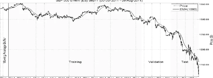
Twenty-four days worth of ES market data (6th July – 8th
August) was used to train, validate and test the HTM classifiers. The first day, 6th July, was used as a buffer for
stabilizing the moving average calculations (used to create lagging market trend indicators), the first 70% (7th – 28th
July) of the remaining 23 days was used to train the classifiers, the following 15% (29th – 3rd August) was used
to validate the classifiers and the last 15% (3rd – 8th August)
was used to test them. The dataset is depicted in Fig 1.
Since the test set (3rd – 8th August) demonstrated a
bearish market trend, additional market data (9th August –
1st September) was downloaded, containing a horizontal
market trend (15th – 17th August) and a bullish market trend
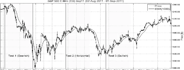
(23th – 25th August). Fig 2 displays the three test sets chosen in order to test the classifiers. The 1000-period exponential moving average, EMA(1000), is plotted in the figure together with the closing price for each 1-minute bar. For the minute-resolution used in this paper, the EMA(1000) can be considered a long term trend.
Test set 1 shows a bearish market trend, where most price action occurs below the long-term trend. This downtrend should prove challenging for classifiers based solely on a buy-and-hold trading strategy. Although, a properly trained model should be able to profit from trading the volatility in the market. The closing price shows a high degree of market volatility between 5-8 August.
Test set 2 shows signs of a horizontal market, in which the long term trend displays a flat price development. In the horizontal market, the long term trend is mostly centered over the price action. There is plenty of market volatility.
Test set 3 characterizes a bullish market with plenty of volatility. In a bullish market, the price action occurs above the long term trend. Trading the volatility in such a market should be profitable using a buy-and-hold strategy.
B. Preprocessing
The data was aggregated into one-minute epochs (bars), each including the open-, high-, low- and close prices, together with the 1-minute trade volume. Missing data points, i.e. missing tick data for one or more minutes, was handled by using the same price levels as the previous, existing aggregated data point.
Once the raw data had been acquired and segmented into one-minute data, it was transformed into ten technical indicators. These feature sets were then split into a training
set, a validation set and three test sets. The data in each data set was fed to the classifiers as a sequence of vectors, where each vector contained the 10 features. One vector relates to 1-minute of data.
The classification task was defined as a 2-class problem: Class 0 – The price will not increase by at least 2
ticks at the end of the next ten-minute period Class 1 – The price will increase by at least 2 ticks
at the end of the next ten-minute period
A tick is the minimum amount a price can be incremented or decremented for the specific market. For the S&P 500 E-mini index futures contract (ES), the minimum tick size is 0.25 points, where each tick is worth $12.50 per contract.
The trading strategy utilized was a simple buy-and-hold, i.e. if the market is predicted to rise with at least 2 ticks at the end of the next ten minutes, then buy one lot (contract) of ES, hold it for 10 minutes, and then sell it at the current price at the end of the 10-minute period.
Confusion matrices were used to monitor performance: False Positive (FP) – algorithm incorrectly goes long
when the market moves in the opposite direction. True Positive (TP) – algorithm correctly goes long
(buys) when the market will rise by at least 2 ticks at the end of the next 10-minute period.
False Negative (FN) – algorithm does nothing when it should go long (buy), i.e. a missed opportunity. True Negative (TN) – algorithm correctly remains
idle, therefore avoiding a potential loss.
A simple performance measure, the rate between winning and losing trades, was derived from the confusion matrices. This measure, the ratio between TP and FP (TP/FP), was used to measure classifier performance. Another relevant measure is PNL, the profit made or loss incurred by a classifier. These, somewhat unconventional, measures were adopted from [23] for comparison purposes.
C. HTM Configuration
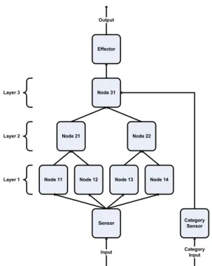
Configuring an HTM as a binary classifier entails providing a category (class) vector along with the feature vector during training. For each feature vector input there is a matching category vector that biases the HTM network to treat the current input pattern as belonging to one of the two classes; 0 or 1. Obviously, during inference mode, the HTM network does not use any category input. Fig 3 shows an HTM with 3 layers configured as a classifier.
The set of feature vectors were fed to the HTM’s sensor, whereas the set of class vectors (category input) were fed to the category sensor during training. The top-level node receives input from the hierarchically processed feature vector and from the class vector via the category sensor. The output from the top-level node is either class 0 or 1. Developing an HTM is an iterative process in which parameters are refined to produce a more accurate classifier. The 4 HTM parameters considered were:
Maximum Distance - the sensitivity, in Euclidean distance, between two input data points.
Network Topology – a vector, in which each element is the number of nodes in each HTM layer.
Coincidences - the maximum number of spatial patterns an HTM node can learn.
Groups – the maximum number of temporal patterns an HTM node can learn.
The network topology setting is self-explanatory, but the other three parameters warrant a further explanation. During training, similar and frequently occurring spatial patterns are grouped together to form clusters, in which the cluster centers are called coincidences in HTM terminology.
Likewise, frequently occurring sequences of spatial patterns (or coincidences to be more precise) are grouped together to form temporal groups. Patterns in the same group are likely to follow each other in time. During inference, spatial patterns are compared to cluster centers (coincidences), where the Maximum Distance parameter setting determines how close (similar) a spatial pattern must be to a specific cluster center in order to be considered part of that cluster. For example, with the maxDistance setting as shown in Fig 4, pattern Pa belongs to cluster center C1. If maxDistance is
gradually increased, pattern Pb will eventually be considered
as part of the cluster too.
The choice of HTM parameters, training method and performance measures were borrowed from Aslin [23].
D. Experiments
The initial HTM experiments targeted the maxDistance parameter, which was varied from 0.001 to 0.5. The classifier with the best compromise between highest profit and TP/FP ratio was chosen for the remaining experiments (this is obviously not the optimal solution, since the optimal
maxDistance setting will vary slightly with the network
topology, but to keep the method simple this approach was adopted from [23]).
In the second set of experiments, the network topology was varied while keeping the number of coincidences and groups constant. Four 2-layer, nine 3-layer and sixteen 4-layer network topologies were used in the topology experiments. Two classifiers from each network topology order (highest profit and TP/FP ratio respectively) were chosen for the third set of experiments.
The number of coincidences and groups were varied during the third set of experiments. The same configuration per layer was used for both the coincidences and the groups. The HTM model with the highest TP/FP ratio was selected for the testing phase.
In order to benchmark the HTMs against a well known machine learning technology, multiple ANNs were created using the pattern recognition neural network (PATTERNNET) toolbox in MATLAB (R2011a). The invariant part of the ANN configuration consisted of a feed-forward network using the scaled conjugate gradient training algorithm [26], mean squared error (MSE) performance measure and a sigmoid activation function in the hidden- and output layers. These default settings were
Node 21 Node 31
Node 22
Node 11 Node 12 Node 13 Node 14
Effector Category Sensor Sensor Input Output Category Input Layer 1 Layer 2 Layer 3
Fig. 3. HTM network configured as a classifier.
X Y Pa Pb C1 Max Distance
considered appropriate according to [27]. The only variable configuration parameter considered in the ANN experiments was the network topology, including 10 runs per topology with different, randomly initialized weights and biases. The ANN model with the highest TP/FP ratio during the validation phase was chosen for the testing phase.
In the final tests, the candidate HTM and ANN models from the validation phase were tested on the three test sets. Contrary to the training and validation phases, a fee of $3 per contract and round trip was deducted from the PNL to make the profit and loss calculations more realistic, since an overly aggressive model incurs more fees (this penalty was a late addition, and should really have been incorporated from the beginning, i.e. while optimizing in the parameter space).
V. RESULTS
Unless specified, all tables below include the columns;
No (model number), Topology (HTM network topology), Coincidences & Groups (maximum number of coincidences
and groups a node can learn per layer), TP/FP (ratio between true- and false positives), PNL (profit and loss).
A. Max Distance
Nineteen models were trained and validated with different maxDistance settings. Table I shows three models from the validation phase; model 1.1 yielding the highest profit, model 1.3 with the highest TP/FP ratio and model 1.2 with the best compromise between the two performance measures. The maxDistance setting of 0.005 for model 1.2 was chosen for the remaining experiments.
B. Network Topology
Twenty-nine models were trained and validated with different network topologies (2-4 layers). Table II shows the six models with the best performance scores from the validation phase. Two models from each network topology order were selected. Models 2.2, 2.4 and 2.5 demonstrated the highest profits and models 2.1, 2.3 and 2.6 the highest TP/FP ratios within their topology order. These six models were selected for the coincidences and groups experiments.
Comparing the performance measures between the training- and validation sets, showed that a high node count in each layer resulted in over-fitting, i.e. a substantial drop in performance between the training- and validation sets.
C. Coincidences and Groups
Using the six models obtained from the topology experiments, fifty 2-layer, seventy 3-layer and over a hundred 4-layer models were trained and validated with different settings for their coincidences and groups. The two models with the best performance, one with the highest profit and one with the highest TP/FP ratio, from each of the six network topologies are presented in Table III.
One 2-layer and one 3-layer model had both the highest profit and TP/FP ratio, yielding ten models in total. Models 3.1 and 3.5 were eliminated due to their low transaction tendencies (e.g. model 3.5 only had 6 TPs and 1 FP). In fact, any model with a transaction rate under 1% was eliminated (this penalty was a late addition, and should really have been incorporated from the beginning, i.e. while optimizing in the parameter space). The remaining model (3.4) with the highest TP/FP ratio was chosen as the candidate model for the final set of tests.
Comparing the performance measures between the training- and validation sets, showed that a high number of coincidences and groups resulted in over-fitting. Conversely, a low number resulted in under-fitting.
D. ANN Validation Results
The PATTERNNET command in MATLAB (R2011a) was used to create benchmark ANN models using the same training and validation sets. The validation results of the six best ANN models (two from each network topology) are shown in Table IV. Models A.1-3 and A.5 had low transaction tendencies and were therefore eliminated. Model A.6 was chosen as the candidate ANN model.
TABLEI
HTM MAXDISTANCE VALIDATION RESULTS
No Coincidences & Topology + Groups MaxDistance TP/FP PNL 1.1 [10,2] [512,256] [0.001,0.001] 0.917 $2612.50 1.2 [10,2] [512,256] [0.005,0.005] 1.087 $2350.00 1.3 [10,2] [512,256] [0.5,0.5] 1.500 $237.50 TABLEII
HTMTOPOLOGY VALIDATION RESULTS
No Topology Coincidences & Groups TP/FP PNL
2.1 [10,2] [512,256] 1.087 $2350.00 2.2 [10,10] [512,256] 0.879 $3675.00 2.3 [10,10,1] [512,256,128] 0.750 (-$50.00) 2.4 [10,10,10] [512,256,128] 0.581 $1137.50 2.5 [10,10,10,2] [512,256,128,128] 0.581 $412.50 2.6 [10,10,10,10] [512,256,128,128] 0.607 $250.00 TABLEIII
HTMCOINCIDENCES &GROUPS VALIDATION RESULTS
No Topology Coincidences & Groups TP/FP PNL
3.1 [10,2] [256,128] 3.500 $2950.00 3.2 [10,2] [1024,64] 1.077 $5762.50 3.3 [10,10] [1024,512] 1.118 $8937.50 3.4 [10,10,1] [128,128,64] 1.261 $1325.00 3.5 [10,10,1] [1024,256,256] 6.000 $200.00 3.6 [10,10,10] [64,64,64] 1.059 $3975.00 3.7 [10,10,10,2] [128,128,128,128] 0.753 $3525.00 3.8 [10,10,10,2] [1024,512,256,128] 0.606 $3950.00 3.9 [10,10,10,10] [512,512,64,64] 0.613 $850.00 3.10 [10,10,10,10] [512,512,512,512] 0.599 $1212.50
E. Testing the Models in Three Market Trends
The candidate HTM and ANN models were exposed to three test sets; a bearish (set 1), a horizontal (set 2) and a bullish market (set 3). $3 per contract and round trip was deducted from the PNL to make the profit and loss calculations more realistic. The results are presented in Table V, where the accumulated PNL is shown in column
ACC PNL.
The results show that the HTM model was profitable in all three market trends whereas the ANN model struggled in the bearish market. The HTM model also demonstrated good TP/FP ratios with little decay from the training- and validation sets (only the ratio for the bullish market was lower than 1.00). Thus, the HTM models generalized well. More erratic behavior was observed for the ANN model.
F. HTM Parameter Settings
Observations made during the training- and validation phases show the importance of choosing the correct set of parameter settings for the HTM network. The maxDistance setting, network topology and the number of coincidences and groups all have a great impact on classifier performance. By choosing a low value for the coincidences and groups, the HTM model lacks enough memory to learn spatial and temporal patterns efficiently. Conversely, choosing a high value leads to over-fitting, where the HTM model’s performance is high in the training phase but shows a substantial degradation in the validation phase. This relationship was also evident during the network topology experiments, where a high number of layers, and nodes in each layer, resulted in classifier over-fitting.
VI. CONCLUSION AND FUTURE WORK A. Conclusion
The results show that the Hierarchical Temporal Memory (HTM) technology can be used together with a feature vector of technical indicators, following a simple buy-and-hold trading strategy, to create a profitable trading algorithm for financial markets. With a good choice of HTM parameter values the classifiers adapted well to novel data with a minor decrease in performance, suggesting that HTMs generalize well if designed appropriately. Indeed, the HTMs learned spatial and temporal patterns in the financial time-series, applicable across market trends. From this initial study, it is obvious that the HTM technology is a strong contender for financial time series forecasting. Results also suggest that HTM performance is at the very least comparable to commonly applied neural network models.
B. Future Work
This initial case study was intended as a proof of concept of using the HTM technology in algorithmic trading. Therefore, an overly simplistic optimization methodology was utilized and primitive evaluation measures employed. Only a small subset of the HTM's parameter set was considered in the optimization process. Furthermore, the penalizing of excessive models, with either too aggressive- or modest trading behavior, was applied after the training phase. Finally, the ANNs, used as the benchmark technology, were trained using the default parameter settings in MATLAB. A more meticulous tuning process needs to be applied to the neural networks in order to justify explicit comparisons between ANNs and HTMs.
A future study will address these shortcomings by employing an evolutionary approach to optimizing a larger subset of the HTMs' and ANNs' parameter sets simultaneously, while utilizing standard evaluation measures, such as accuracy, precision, recall and F1-measure. Excessive models will be penalized in the parameter space.
REFERENCES
[1] E. Fama, "The Behavior of Stock-Market Prices," The Journal of
Business, vol. 38, pp. 34-105, 1965.
[2] E. Fama, "Efficient Capital Markets: A Review of Theory and Empirical Work," The Journal of Finance, vol. 25, pp. 383-417, 1970.
[3] W. P. Hamilton, The Stock Market Barometer: Wiley, 1998. [4] R. Rhea, The Dow Theory: Fraser Publishing, 1994.
[5] J. Murphy, Technical Analysis of the Financial Markets: New York Institute of Finance, 1999.
[6] P.-N. Tan, et al., Introduction to Data Mining: Addison Wesley, 2009. [7] J. Hawkins and S. Blakeslee, On Intelligence: Times Books, 2004. [8] D. George and B. Jaros. (2007, The HTM Learning Algorithms.
Numenta Inc. Available:
http://www.numenta.com/htm-overview/education/Numenta_HTM_Learning_Algos.pdf [9] J. Hawkins and D. George. (2006, Hierarchical Temporal Memory -
Concepts, Theory and Terminology. Numenta Inc. Available:
http://www.numenta.com/htm-overview/education/Numenta_HTM_Concepts.pdf TABLEIV
ANNVALIDATION RESULTS
No Topology TP/FP PNL A.1 [10,10] 9.000 $945.00 A.2 [10,10] 2.800 $1580.50 A.3 [10,1,1] 4.500 $879.50 A.4 [10,10,10] 1.164 $4015.50 A.5 [10,10,5,1] 6.000 $991.50 A.6 [10,10,10,2] 2.500 $1745.00 TABLEV TEST RESULTS
No Test Set TP/FP PNL ACC PNL FEES
3.4 1 ↓ 1.145 $2687.50 $2687.50 $399.00 2 ↔ 1.162 $1487.50 $4175.00 $240.00 3 ↑ 0.776 $900.00 $5075.00 $261.00 A.6 1 ↓ 1.062 (-$1900.00) (-$1900.00) $600.00 2 ↔ 5.500 $1250.00 (-$650.00) $39.00 3 ↑ 0.909 $762.50 $112.50 $63.00
[10] D. George, et al., "Sequence memory for prediction, inference and behaviour," Philosophical transactions - Royal Society. Biological
sciences, vol. 364, pp. 1203-1209, 2009.
[11] D. George and J. Hawkins, "Towards a mathematical theory of cortical micro-circuits," PLoS Computational Biology, vol. 5, p. 1000532, 2009.
[12] J. Pearl, Probabilistic reasoning in intelligent systems: networks of
plausible inference: Morgan Kaufmann, 1988.
[13] Numenta. (2011). NuPIC 1.7.1. Available: http://www.numenta.com/legacysoftware.php
[14] V. Mountcastle, "An Organizing Principle for Cerebral Function: The Unit Model and the Distributed System," V. Mountcastle and G. Edelman, Eds., ed Cambridge, MA, USA: MIT Press, 1978, pp. 7-50. [15] D. George and J. Hawkins, "A hierarchical Bayesian model of invariant
pattern recognition in the visual cortex," in Neural Networks, 2005.
IJCNN '05. Proceedings. 2005 IEEE International Joint Conference on, 2005, pp. 1812-1817 vol. 3.
[16] J. Thornton, et al., "Robust Character Recognition using a Hierarchical Bayesian Network," AI 2006: Advances in Artificial Intelligence, vol. 4304, pp. 1259-1264, 2006.
[17] J. V. Doremalen and L. Boves, "Spoken Digit Recognition using a Hierarchical Temporal Memory," Brisbane, Australia, 2008, pp. 2566-2569.
[18] J. Thornton, et al., "Character Recognition Using Hierarchical Vector Quantization and Temporal Pooling," in AI 2008: Advances in Artificial
Intelligence. vol. 5360, W. Wobcke and M. Zhang, Eds., ed: Springer
Berlin / Heidelberg, 2008, pp. 562-572.
[19] S. Štolc and I. Bajla, "On the Optimum Architecture of the Biologically Inspired Hierarchical Temporal Memory Model Applied to the Hand-Written Digit Recognition," Measurement Science Review, vol. 10, pp. 28-49, 2010.
[20] J. Maxwell, et al., "Hierarchical Sequential Memory for Music: A Cognitive Model," International Society for Music Information
Retrieval, pp. 429-434, 2009.
[21] D. Rozado, et al., "Optimizing Hierarchical Temporal Memory for Multivariable Time Series," in Artificial Neural Networks – ICANN
2010. vol. 6353, K. Diamantaras, et al., Eds., ed: Springer Berlin /
Heidelberg, 2010, pp. 506-518.
[22] D. Rozado, et al., "Extending the bioinspired hierarchical temporal memory paradigm for sign language recognition," Neurocomputing, vol. 79, pp. 75-86, 2012.
[23] F. Åslin, "Evaluation of Hierarchical Temporal Memory in algorithmic trading," Department of Computer and Information Science, University of Linköping, 2010.
[24] CME. (2011). E-mini S&P 500 Futures. Available:
http://www.cmegroup.com/trading/equity-index/us-index/e-mini-sandp500.html
[25] Slickcharts. (2011). E-mini Futures. Available: http://www.slickcharts.com
[26] M. F. Møller, "A scaled conjugate gradient algorithm for fast supervised learning," Neural Networks, vol. 6, pp. 525-533, 1993.
[27] G. Zhang, et al., "Forecasting with artificial neural networks:: The state of the art," International Journal of Forecasting, vol. 14, pp. 35-62, 1998.