Nr 196 - 1993
Comparison of partial and general equilibrium analysis of benefits from a road improvement
Imdad Hussain
Paper prepared for The Fourth CGE Modeling Conference to be held on October 28-30, 1993 at the University of Waterloo, Ontario, Canada
VTl särtryck
Nr 196 - 1993
Comparison of partial and general equilibrium analysis of benefits from a road improvement
Imdad Hussain
Paper prepared for The Fourth CGE Modeling Conference to be held on October 28-30, 1993 at the University of Waterloo, Ontario, Canada
Väg- och Trafik-/
Ins'Z'tutet
COMPARISON OF PARTTAL AND GENERAL EQUILIBRIUM
ANALYSIS OF BENEFTTS FROM A ROAD IMPROVEMENT
by Imdad Hussain
Swedish Road and Transport Research Institute
S - 50195 Linköping, Sweden
THE PAPER PREPARED FOR THE FOURTH CGE MODELING CONFERENCE
TO BE HELD ON OCTOBER 28 - 30, AT THE UNIVERSITY OF WATERLOO,
COMPARISON OF PARTIAL AND GENERAL EQUILIBRIUM ANALYSIS OF BENEFITS FROM A ROAD IMPROVEMENT
by Imdad Hussain
Swedish Road and Transport Research Institute, S - 581 95 Linköping, Sweden Phone no. Int + 46/2041 73. Telefax no. Int + 46/20 43 80
( September, 1993 )
ABSTRACT
Since the 19505 the CBA has been used in the appraisal of road schemes in a more or less similar shape as it is applied in the known practical manuals today. Transport cost savings for existing traffic completely dominate the welfare side of the benefit
calculation models used in road planning in various countries. However, it is widely beleived that substantial benefits beyond the transport cost savings may arise in the form of industrial growth and employment. This paper attempts to analyse this issue by using an applied general equilibrium model of a regionalized economy, integrating goods and passenger traffic in the model. A comparison of transport cost savings for goods and passenger traffic and general equilibrium benefit measure of equivalent variation is made to note the gap between the two measures. The paper also pinpoints the conditions for making the gap larger.
1. INTRODUCTION
The measurement and evaluation of benefits likely to arise from an investment in transport infrastructure may be primarily motivated in order to make decisions about the total amount of investment in a transport project, which could be justified in pursuit of the efficient allocation of available resources. When there are no indivisibilities and externalities and no public good cases and other price distorting market imperfections in an economy, the ordinary cost-revenue-analysis approach based on marginal cost pricing will suffice for measuring the social costs and total net benefits of a public road
investment [ Friedlaender , 1965 ]. However, the economic conditions similar to those referred to in the above hardly exist in real world economies. Therefore, the so called competitive optimum rule of setting price equal to marginal cost of a service or good usually may not be applicable while assessing the social desirability of a public transport investment 1.
Moreover, investments in new road networks or in existing road improvement projects often claim large amounts of resources. Besides that such investments also happen to be of an irreversible character. This makes a rather correct knowledge of demand for services of such facilities, and an estimate of all possible benefits which may accerue to the investment in question, a rather compelling necessity. It may also be remembered that users of road services simultaneously contribute in the production of these services and in this process they impose costs on themselves and on other users. Under such conditions an efficient road investment policy will be the one which gives rise to maximum net social benefits for the society as a whole [Jansson , 1984].
The efficiency and financial cost covering considerations of a road investment project, typically give rise to an intricate discussion about the problems of road pricing and thus the computation of optimal road user charges. The essence of the theory of road user's charges is that if the price paid for the services of a road reflects its cost of provision, then the resources will be efficiently distributed among the use of road and consumption of other commodities and services 2. However, an interesting question in this regard is whether the services of a road can be regarded as a public good or not. The important conclusion of the theory suggests that optimal road user charges usually do not provide full coverage of investment costs to a road authority 3,
The economic system has the property that "everything depends upon everything else". This suggests that in a simultaneous consideration of costs and benefits the size of benefits from a road investment will also depend upon what kind of charges and taxes are raised in order to finance the investment. Since different types of charges and taxes lead to different levels of price distortions in the economy, the size of net benefits would vary according to the chosen tax regime. Therefore, in a more realistic scenario, the benefits of an investment ought to be seen with due consideration to the cost of
investment and how this cost is allocated among different individuals and groups in the society. However, as a practical rule the assessment of benefits is in general made independently from the cost of investment. A formal comparison of the investment cost and the benefits is then made as the last step of the evaluation and decision making process.
2. THE PROBLEM
The economic theoretic principles implied by the practical CBA of road investments have been derived from the theory of welfare economics 4. The core idea of the theory behind these methods suggests that total willingness of users to pay for a new facility or
for an upgrading investment in transport system may be seen to represent the true magnitude of its socio-economic benefits. Formally this type of analysis requires the specification of suitable transport demand models. However the practical road appraisal manuals recognize the absence of a system of pricing the services of roads in the
ordinary sense of economic theory. Therefore, in the absence of transport demand models, traditional transport cost models based on generalized transport cost approach are used to estimate the social rate of return in the real world appraisal of transport investments 7. As a consequence the benefits of a road investment are estimated by measuring transport cost savings for exsisting or initial traffic, in connection with road planning in different countries. These benefits in fact completely dominate the welfare side of the road appraisal manuals. Take for example, OBJEKTANALYS and COBAS. Transport costs in this particular context are comprised of various user cost components. The most important components entering in the costs account are : traffic accident cost, travel time cost, vehicle operating cost and cost of discomfort due to the journey taken'.
Note that the negative externalities of road traffic in terms of increased polution of air, noise and deterioration of natural beauty may possibly also be included as components of the generalized cost to the extent these can be quantified and evaluated [ see Mishan, 1966]. However, such cost factors are not explicitly considered in the appraisal manuals used in practise. It may also be mentioned that the cost elasticity of the volume of transport is believed to be very low and therefore, any possible gains associated with increased traffic or newly generated traffic are neglected in the practical appraisal manuals. In the usual transport planning jargon, the benefit analysis is said to have based on fixed trip matrix approach. Which means that the volume of traffic is assumed to remain unchanged after the road improvement, as visible changes in traffic volume are usally assumed to be taking place only through the shifts in route assignment 8, Consequently, transport cost savings for initial traffic are regarded to be a reasonable approximation of the total net welfare gains for the society as a whole. The issue concerning the true appraisal of investments in road infrastructure has been in the focus for many studies, using various types of models and methods, in several countries of the world. Due to the cross-disciplinary nature of this problem, researchers from different scientific disciplines have been contributing to the growth of knowledge in this area. However, every discipline has had the tendency to consider the complexities of the problem in a somewhat different perspective. Some important examples of the research in the area of transportation and economic development are: Tinbergen (1957), Bos and Koyck (1961), Friedlaender (1965), Brown and Harral (1965), Wilson et al (1966), Mohring and Williamson (1969), Cleary and Thomas (1973), Dickey and Sharpe (1974), Dodgson (1974), Peaker (1976), Thornton (1978), Friedlaender and Spady
(1981), Sasaki (1983), Liew and Liew (1984), Dodgson (1984), Kanemoto and Mera (1985), Mackie and Simon (1986), Quarmby (1989), Aschauer (1989), Anderstig and Mattson (1989), Peterson (1989), Binder (1989), Forkenbrock and Foster (1990),
Hulthen (1991) and Weisbrod and Beckwith (1992). In fact the only safe conclusion that can be drawn from these references is that the opinions among the researchers, about the existence and magnitude of development effects and how they should be treated in the evaluation process, are still very much divided.
In some studies referred to in the above, the view has been expressed that investments in road transport infrastructure may give rise to substantial benefits over and above the traditional measure of transport cost savings for existing traffic. Road investments in most of these studies are considered to be qualitatively and quantitatively unique as compared to other investment activities in a national or regional development
programg-Extra benefits of road investments are believed to arise due to their perceived impact on
the growth of industrial productivity and possibly increased employment level in the
economy.
Then the important question is whether there is something crucial, from the welfare
point of view of a society, that the practical benefit calculation models have been
omitting in the appraisal of transport investments. How important could be the gains
associated with prospective newly generated traffic ? In order to be more specific the
problem can be split in three separate parts :
(i ) Is the traditional measure of transport cost savings a reasonable approximation of
all benefits which may accerue to a road investment?
( ii ) How important are the welfare gains associated with newly generated traffic.
( iii ) Given that the welfare gains associated with newly generated traffic have also
been identified, quantified, evaluated and added to transport cost savings for existing
traffic. Could there be still more benefits over and above this extended measure, which
must be taken into account in the welfare analysis of a road investment ?
Now the thesis that infrastructural road investments will play an important role in the
economic development of countries and regions with largely unexploited resources, has
been agreed upon in general. A careful passage through the course of economic history
reveals that transports, during the earlier stages of the economic development, formed a
bottleneck hindering industrial expansion. Smaller markets for final goods and limited
access to natural resources at that time were obvious causes of the slowness of speed
and inadequate capacity of transport system. This phenomenon thus excercised a hard
break on the growth of economic activity 10, Therefore, the large scale investments in
transportation infrastructure at that stage naturally facilitated on one hand, the access to and exploitation of otherwise idle natural resources, and on the other helped extending markets for agricultural and industrial products. That process, in turn, lead to economies of scale and specialization in the production of industrial goods. Under such economic conditions, transport cost savings for existing traffic plus gains to generated traffic will usually underestimate the true size of economic benefits which may arise due to a road investment [ Friedlaender , 1965 ].
Whether the same phenomenon could still exist in the case of mature and developed economies with almost full employment of resources, is a question that still lacks a clear answer. A rather usual problem faced by the contemporary modern economies seems to have been the underutilization of existing industrial capacity. Therefore, opinions about the long-standing issue of the nature and size of socio-economic effects of large scale investments in transport infrastructure, in developed countries, are in fact much divided.
3. PERCEPTIONS ABOUT THE NATURE OF BENEFITS
For any one concerned with the task of road investment appraisal the following three stage arrangement may be the point of departure :
(i) To identify all possible effects of a transport investment, for example, of a new road investment or of an investment aimed at the qualitative improvement, repair and maintenance of old transport infrastructure.
(11) To quantify all the effects. ( i1 ) To evaluate all the effects
In principle the effects of an investment in transport infrastructure may be considered in a local, regional or a national perspective. This in turn requires a detailed analysis of the problem which would litterally speaking lead one to strife for capturing of innumerable effects of different types and nature. An added difficulty is raised by the absence of general rules to determine the level of detail in the course of analysis. The practical road appraisal manuals in use consider transport cost savings for existing traffic adjusted for some environmental effects as a measure of total benefits accruing to a road investment. This practice has been useful for empirical impact studies with regard to user cost aspects of the problem such as accessibility, traffic safety and vehicle costs etc . Nevertheless, a thorough understanding of any prospective effects over and above transport cost savings for existing traffic has been difficult to reach within the framework of these manuals. In fact there has not even been a generally agreed upon nomenclature used to describe the full range of effects of different types. For example, the prospective impact which a road investment may have on the possible economic
development of regional and national economies, have been mentioned in the literature using different terminologies.
Some examples are: "Indirect Benefits" [ Tinbergen (1957), Bos and Koyck (1962) and Friedlaender (1965) ], "Indirect and Secondary Benefits" [ Margolis (1957) and
Gwilliam (1970) ], "External Benefits" [ Brown and Harral (1965) ], "Reorganization Benefits" [ Mohring and Williamson (1969) ] and "External and Secondary Benefits" [ Dodgson (1973) ] and "Development Effects" [ Keuhn and West (1971) and Weisbrod and Beckwith (1992) ]. In more recent research in this area several other designations have been used to emphasize the nature of such effects. These are for example, System Effects, Network Effects, Synergy Effects, Growth Effects, Dynamic Effects and Nonuse Values etc. [ See for example, Andersson and Strömquist (1988), Aschauer (1989) and (1990), Petersson (1989), Westin (1990), Lundqvist (1991), Johansson (1992) and Tapper (1992) ]. To the extent such effects are present and can genuinely be identified, quantified and given a value, it may be important to take them into account in terms of net welfare gains to the society as a whole. The emergence of such effects is beleived to depend on changes in the pattern of resource allocation, relocation in space of economic activities and changes in overall productivity of an economic system. In this study the term "development benefits" will be used to cover all those positive effects of a road investment which may arise beyond the benefit measure of transport cost savings for existing traffic.
Regarding the assertion that, road investments in addition to transport cost savings for existing traffic also give rise to substantial development benefits, three major arguments have usually been put forward in the relevent litterature :
(i ) It has been argued that cheaper transports in relation to other inputs used by some industries, will generally lead to the substitution of transports for some other kinds of the production outlays. In particular, if production is characterized by economies of scale a reduction in the cost of distribution may induce the industry to concentrate its production in fewer but larger plants, thus materializing the benefits due to economies of scale in production. Mohring and Williamson (1969) have analysed this aspect of the problem taking the example of a firm operating under the conditions of monopoly. The main conclusions of their study are that total gains to the industry arising through such a spatial reorganization of the production plants may be measured by considering the change in area to the left of transport demand curve for the firm. Dodgson (1984) has considered the similar problem although for a firm operating under perfect competition. He reached the similar conclusion to that drawn by Mohring and Williamson (1969) and has used a different name for their "reorganization benefits" expressing such benefits as "benefits due to newly generated traffic". Similar views have also been expressed by
other researchers. In particular, they confirm that the above conclusions may be true when the scale of the transport investment is very small. This is because induced changes in prices under such cases may cancel out each other. Whether the similar conclusions may also be drawn in case of large scale transport investments, has not been thoroughly investigated [see Harberger (1971) , Boadway (1975) and Lesourne (1975)].
( ii ) The second argument is that in case production of commodities requires transport of intermediate goods so that transport service itself becomes an intermediate input, then any reduction in the transport cost of the intermediate goods will cause the relative prices of final goods in the economy to change. These price changes will in turn bring about further variations in the structure of production and consumption in the economy, with a subsequent impact on the level of welfare in a society. The traditional benefit measure of transport cost savings for existing traffic, it has been argued, can not grasp the benefits associated with such allocational changes in the economic structure. This aspect of the benefit assessment problem suggests an investigation of the welfare impact of such changes in a comprehensive general equilibrium analysis of the economy in question. Such attempts have been made before by researchers such as: Tinbergen (1957), Bos and Koyck (1961), Liew and Liew (1984) and Kanemoto and Mera (1985).
( iii ) Thirdly, the view has occasionally been expressed by some researchers in this area that the traditional practice of measuring benefits in terms of transport cost savings is based on a static type of analysis and therefore, it can not take into account the benefits which may be identified in a dynamic analysis of the investment. It has been established by the researchers that regional patterns of economic activity response to changes in transport infrastructure only at a very low pace [Mackett (1985) and Lundqvist (1991)].
By the notion "dynamic effects" in this context is usually understood as a positive effect on the overall productivity of production system in an economy. In fact, such views seem to have been fetched from the economic historical argument emphasizing that at the early stages of industrial growth and expansion, innovations in the transport system played a very important role in transforming industrial structures of the developing economies of that time. Transport improvements in such models are usually assumed to generate a positive technological externality, which may result into an increment in the overall productivity1 ! of the production system. However, the causal relationship assumed between transport infrastructure and industrial productivity in this type of analysis has not been accepted in general. But even if transport infrastructure could be established as key determinant of growth in the industrial productivity, the large scale investments in transport infrastructure can not be able to repeat the early processes of
industrial transformation in general. [ Wilson (1986), Binder (1989), Aschauer (1990), Forkenbrock and Foster (1990) and Winston (1991) ].
The controversy over the nature and magnitude of the benefits accruing to a transport improvement makes it necessary that the problem be considered within two different scopes of analysis : ( i ) a partial equilibrium analysis by looking at transport cost savings and gains to generated traffic due to a transport improvement and ( ii ) an analysis of the problem using a general equilbrium approach where the benefits are measured in terms of equivalent variation.
This study is based on a comparative static analysis of the benefit assessment problem and attempts to make its contribution by using the framework of an interregional computable general equilibrium model ( ICGFE ). As a first step in this direction the analysis is conducted under the usual assumptions of a perfect market economy framework. The analysis is then extended to conditions of different kinds of market imperfections and the possibility of interregional commuting. The analysis ends up into the comparison between the partial- and the general equilibrium measures of benefits due to different degrees of transport cost reductions.
4. THE MODEL
The model used in this study considers an economy with two final goods, two factors of production and two geographically separated regions. According to the conditions of the model the homogeneous consumer group in one region owns all the capital while the consumer group in the other region has the only endowment of all the available labour [ This phenomenon may be interpreted in terms of "rich" consumers and "poor" consumers as has been done in Shoven and Whalley, 1984 ].
Further the model assumes that the consumers do not have any initial endowments of goods. Suppose that the production of both consumer goods takes place in the region which supplies capital, henceforth called region 1. Each good is produced according to a Cobb-Douglas constant-returns-to-scale production function. The consumer preferences in both regions are characterized by the usual Stone-Geary type of utility functions and the consumer demands in the model are derived through maximizing the consumer utility subject to respective budget constraints. It is also assumed that consumers in region 1 demand both goods whereas the consumers in region 2 [the region supplying the labour force] consume one of the consumer goods - good 1 - and demand also leisure. Good 1 is therefore demanded in both regions for consumption, although good 2 is only consumed in region 1.
The transportation of good 1 from region 1 to region 2 gives rise to a transport cost which is incurred by the consumers in region 2. The unit transport cost of the good is given by a transportation coefficient. This coefficient is equivalent to the money value of a certain amount of good 2
multiplied. by its price. However, in this model
good 2 is treated as a numeraire and therefore, the transportation coefficient and
the unit transport cost accounted in monetary units become one and the same
thing.
Since the production of both goods, according to the assumption of the model,
takes place in region 1, the consumers in region 2 - supplying the labour - must
commute to region 1 to be able to work. The cost of the passenger trip is usually
measured in generalized cost terms which is traditionally expressed in time units
instead of a monetary value [ For the detailed discussion about the generalized cost
term and the various travel time components etc the reader may be recommended
to see Jansson (1984) and Jansson (1991)]. Consequently, the amount of the time
devoted to commuting during a production period may be expressed as a fraction
of total time endowment. Provided that a transportation system improvement leads
to a reduction in the amount of time spent on commuting the time saved in this
way can be used in production and for leisure. The value of the time savings in the
commuting may then be compared with the general equilibrium benefits of the
transport improvement measured in terms of the equivalent variation. How to
determine the relative value of time devoted to different activities, for example,
work, travel and leisure, is certainly an important and difficult question in real life.
For the sake of simplicity, this study uses wage rate as the standard criterion for
the measurement of the value of time spent on all activities.
In case the transport system improvement implies also a reduction in the unit transport
cost for the movement of goods, then the aggregate traffic benefits in terms ay travel
time savings for commuters and transport cost savings for the goods transport could
simultaneously be measured and compared with the general equilibrium benefits. The
section below gives the equations of the interregional general equilibrium model used in
the analysis. The mathematical model uses the following notations:
notations
Uj = utility index for the consumer in region j
Xcij = consumer demand for good i in region j
10
Xij = committed consumption of good i in region j
H,
0. . = committed leisure in region j
= demand for leisure in region j
X: = quantity produced and supplied of good j
distributional parameter in the production function for good j
9 1
L* = endowment of labour
Lj= demand for labour in sector j
K= endowment of capital
Kj = demand for capital in sector j
Pj = producer price of good j
P;; = price of good i in region j inclusive of the relevent transport cost
w = going wage rate in the economy
p = price of the capital
kj = variable coefficient of capital for sector j
lj = variable coefficient of labour for sector j
B; = share of income of region j spent on the consumption of good i
B,; = share parameter for leisure in region j
t= commuting time coefficient
tjj= transport cost coefficient for the movement of good i to region j
5.
EQUATIONS OF THE MODEL
Consumers ( region 1 )
Preferences
Uj = By lf (Xq -X) + Paj in (XC; - X2])
(1)
Pri + Bar = 1
Budget constraint
p K+n- P; X*;; - P9 X*2; = 0
(2)
11
Demand for good 1
X1 = X11+ B1 [p Xj - P2 X2q ]
Demand for good 2
X©21= X2[+ [p K+n- P; X;; - P2 X2] ] Consumers ( region 2 ) Preferences Uj = Bjz In Bpz in (Hg - 02) Bi2+ Bp2= 1 Budget constraint w (1-1) L* - w Hg - P; X"q2 = 0
Demand for good 1
X2 = Xj2 + Bpa/Pp2 [w (1-1) L* - w 09 - Pp ] Demandfor leisure
H = 097 + BhZ/W [w(1-t)L* WOLZ P12X12]
Producers
Factor input coefficients
Good 1 kj = [9;/(1- 9; ) (w /p)]** i - 91 1 = [(1-@1)/@1 ( p/w )]** 9; Good 2 ka = [ q2 / (1 - @2 ) ( w / p )]** 1 - P3 19= [( 1- 92 )/ 92 (p / w )]** 92 (3 ) (4 ) (5) (6) (7 ) (8 ) (9 ) (10 ) (11) (12)
Unit price equations P; = p kj + w l; P = p ka + w ID Factor demand Good 1 Kj = kj Xj Lj = l; Xj Good 2 Ko = kr X2 Lo = 19 X Commodity balance X1= X1 + X*]2 X3= XS +
th
Factor market balance
K = Kj + Ko
L* = Lj +14 +H + tL*
Definition
P12 =Pj +t17 P7
Transport demand
X9= t12 X"q7
12
(13)
(14)
(15)
(16)
(17)
(18)
(19)
(20)
(21)
(22)
(23)
(24)
13
Variables and Parameters
Equations 3 and 4 and equations 7 through 24 above provide a simultaneous system of 20 independent equations in 20 endogenous variables. The model considers P» as a numeraire. The endogenous and exogenous variables of the model are listed below. Endogenous variables
X3 X42 , X1 , X9 , H2 , X1 , X2 . 4 , L9 . 11 . 12 , Kj , KQ , K1 . k2 , P1 , P2 , w , p and P17 .
Exogenous variables
Pri» Bar» P12. Bn2. 91. 92-X11-X21-X12, 02 ,L* , K,t and tj. Numeraire
P> = 1
6. Numerical values of the model inputs
K = 40 L* = 120 t = 0.20 tj = 0.30
B]] = 0.45 Bj = 0.55 Bj; = 0.65 Bpp = 0.35
Q] = 0.6 99 = 0.4 X;j; = 1 X1 = 2
X71 = 2 Mp = 5
7. The benefit measurement
The model is solved by using GAMS / MINOS system and the equilibrium values of the prices, quantities, incomes and utility indices etc have been obtained from the solutions before and after the transport improvement. These values are then used to measure the value of commuting time savings, transport cost savings for existing traffic, gains to generated traffic and the equivalent variation in the relevent cases. The summary of the results obtained from different cases of the benefit analysis are presented in the tables below. A key to the columns follows:
At = change in the commuting time coefficient
At17 = change in the unit transport cost of good 1 from region 1 to region 2 TS = amount
VTS = monetary value of the time savings
TCSG = transport cost savings for initial goods traffic GGTG = gains to newly generated goods traffic
GGT% = gains due to generated traffic as a percentage of GGTG PEG = TCSG + GGTG
14
EV = the general equilibrium benefit measure of equivalent variation TBM = the true benefit multiplier defined by the ratio EV / PEL
8. Summary of the results
First-best economy model with passenger-
land goods
Table 1
transport. Only unit transport cost for goods changes
- At; |- At
TS
|[VTS
|TCSG|GGT |GGT%
|PEG
|PEL
|EV
TBM
G
10 %
0-544 |0-005
0-895
|0- 549 |0-549 |0-552 |1:006
20 %
1-088 [10-020
14821
|1+108 |1:+108 1-121 1-012
30 %
1-632 |0-045
2781
|1:677 |1:677 1-708 1-018
40 %
2+176 |0-082
3:777
|2258 |2:258 |2:313 1:024
File
50 %
2720 [10-131
4809
|2:851 |2:851 |2:937 |1:030 |PSG2
Table 2
First-best economy model with passenger- and goods
transports. Only commuting time coefficient changes
- At12 - At
TS
VTS
|TCSG|GGT |GGT%
|PEG
|PEL
|EV
TBM
G
10 %
2:40 |0-986
0-986 |0-991 1-005
20 %
4:80 |1.952
1.952 1.972 1-010
30 %
7:20 |2:899
2+899 |2:942 |1:015
40 %
9:60 |3:829
3-829 |3:903 1-019
50 % 12:00 |4-741
4741 14-855 1-024
15
Table 3 First-best economy model with passenger- and goods transport. Unit transport cost for goods and commuting time coefficient both change
- Atjg |- At TS VTS |TCSG|GGT |GGT% |[PEG |[|PEL |EV TBM G 10 % 10 % 2400 0-984 |0-544 |0-008 1:458 0-552 |1:536 |1:550 1-009 20 % 20 % 4-800 1:943 |1:088 |0-032 2:953 1+120 [13-063 [3:118 1-018 30 % 30 % 7200 2:88 1:632 |0-073 4-485 1:705 [4585 [4708 1:027 40 % 40 % 9:-600 3:793 [2:176 [10-132 6:057 2:308 16-101 |6:319 1:036 50 % 50 % |12:000 4:685 [2:720 [0:209 7:671 2:929 [7:614 |7:953 |1:045
Table 4 Second-best economy with passenger and goods transports. 25% tax on labour employment. Unit transport cost for goods and commuting time coefficient both change
- Atjg |- At TS VTS |TCSG|GGT |[|GGT% |PEG |PEL |EV TBM G 10 % 10% 2:400 10.792 [10.529 [10-008 1:499 0-537 |1:329 11.380 1-038 20 % 20 % 4-800 1.565 |1:058 |0-032 3.038 1.090 [2.655 [2.780 1:047 30 % 30 % 7:200 2.319 |1.587 |0-073 4.618 1.661 13.980 |4.201 1-055 40 % 40 % 9:600 3.055 |2:116 |0:-132 6.244 2.248 |5.303 5.644 1:064 50 % 50 % 12:000 3.773 |2.645 |0-209 7.915 2.855 |6.628 |7.111 1-073
16
Table 5 Second-best economy with passenger and goods transport. 35% tax on labour employment. Unit transport cost for goods and commuting time coefficient both change
- Atjgq |- At TS VTS |[TCSG|GGT |GGT% |[PEG |PEL |EV TBM
G . 10 % 10 % 2400 0.735 |0.522 |0-008 1.512 0-530 |1:265 1.324 1-047 20 % 20 % 4800 1.452 1:044 |0-032 3.066 1.076 |2.528 |2.669 1-056 30 % 30 % 7-200 2.152 1.566 |0-073 4.664 1.639 |3.791 |4.034 1-064 40 % 40% 9:600 2.835 (2.088 |0:-132 6.307 2.219 |5.054 |5.422 |1:073 50 % 50 % 12-000 3.502 |2.610 |0:-209 7.998 2.818 |6.320 |6.834 1-081
The results of the perfect market economy model where a transport investment leads to a reduction only in the unit transport cost of goods are presented in table 1 above. The TBM multiplier in this case shows values different to 1 for different degrees of the unit transport cost reduction. However, this difference between the partial equilibrium benefit measure PEL and the general equilibrium benefit measure EV is still very small under the assumption of perfect maket framework. For a 50% reduction in the unit transport cost the PEL measure underestimates the EV by 3%. This small deviation between the benefit measures in the case of two regions model seems to have come up due to the possibility of factor substitution. Benefits to generated traffic amount to about 5% of transport cost savings for existing traffic in this case.
The results of the perfect market economy model when a transport investment leads to a change only in the travel time coefficient are shown in table 2. The partial equilibrium measure of benefits in this model is the value of travel time savings VTS which is to be compared with the EV. The model provides very much similar values of the TBM to those achieved in the perfect market model where only the unit transport cost of goods are reduced due to the transport investment. The deviation of the partial measure VTS from EV is very small (about 2.5%) and may be attributed to the possibility of factor substitution in the model. In table 3 the results of the model, when the transport
investment leads to a reduction both in the unit transport cost for goods as well as in the commuting time cefficient, are shown. The model still continues to assume perfect
17
markets. The partial equilibrium benefit measure in this case is comprised of the VTS and the PEG together. The true benefit multiplier TBM in this case acquires slightly higher values than those cases when the changes in unit transport cost and in the commuting time coefficient took place independently from each other. However, the difference between the PELÅL and the EV even in this case is not substantial. For example, the EV measure overestimates the PEL measure by less than 5% for a reduction of 50% in the unit transport cost of goods as well as in the commuting time coefficient. The results of the model show an upward change in the ratio of generated traffic gains to the transport cost savings as compared to the similar ratio computed by the earlier models. For a 50% reduction in commuting time coefficient and unit transport cost of goods the gains to generated traffic amount to about 7.7% of the transport cost savings for existing traffic.
A labour employment tax is now imposed on producers and the tax revenues raised in this way are given back to the consumers in the labour supplying region. The results of this model for cases of a 25% and a 35% labour tax are shown in table 4 and table 5 respectively. The transport investment is assumed to cause a reduction both in the unit transport cost for goods and the commuting time coefficient. It can be seen from table 4 that a 25% labour tax under such conditions leads to about 3% higher values of the TBM for various scales of transport investment. For a 50% simultaneous reduction in the unit transport cost and commuting time coefficient, the EV now overestimates the PEL by slightly more than 7%. For a 35% labour tax the similar figure is about 8%. As in the taxless case the relative significance of gains to generated traffic increases as the scale of transport investment gets larger.
Tables 6 through table 12 below present the results from different cases of the two regions model under the conditions that a possitive technological externality associated with transport investment exists. It has also been assumed in the model that the magnitude of the externality is directly proportional to the size of the transport investment. Thus a proportional shift in the supply of a production factor (capital) has been assumed to take place due to a given transport investment. Such an assumption may be justified on account of the possibility of a transport investment to facilitate access to productive resources which in the the absence of the given transport investment would have remained unexploited. The similar benefit analysis as in the above is then carried out under varying assumptions about the strength of the externality. The summary of the results of this analysis follows:
18
Table 6 The case of externalities.
Only commuting time coefficient changes
10 % reduction in t leads to 1 % shift in capital supply
- Atjg |- At [TS VTS |[TCSG|GGT |GGT% |PEG |[|PEL |EV TBM G 10 % 2:40 |0:990 0-990 1:272 1:285 20 % 480 |1:968 1:968 [2:548 1:294 30 % 7:20 |[2:935 2:935 [3:813 1:299 40 % 9:60 |3:891 3:891 |5:068 1:302 PEC 50 % 12-00 |4-842 4-842 |6-399 1-321 |21 *
Table 7 The case of externalities
Only commuting time coefficient changes
10 % reduction in t leads to 2 % shift in capital supply
- At; 3 - At TS VTS |TCSG|GGT |GGT% |PEG |PEL |EV TBM G 10 % 240 |0-994 0-994 |1:552 |1:561 20 % 4:80 1:984 1:984 |3:118 1:571 30 % 720 |2:973 2973 |4:725 |1:589 40 % 9:60 |3:960 3:960 |6:-346 1-603 PEC 50 % 12:00 |4:945 4:945 [7:967 |1:611 |22 *
19
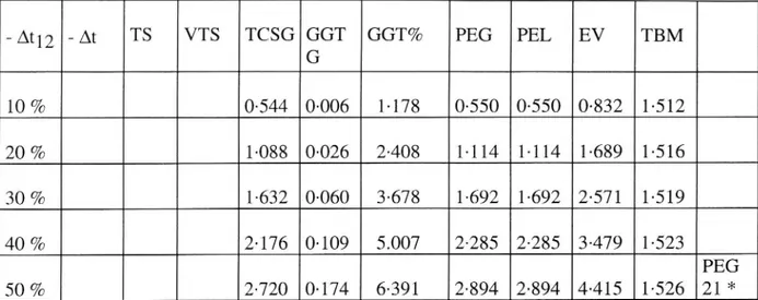
Table 8 The case of externalities
Only unit transport cost for goods changes
10 % reduction in tjz Leads to 1 % shift in capital supply
- Atjg |- At [TS 'VTS [TCSG|GGT |GGT% |[PEG [PEL |EV TBM G 10 % 0-544 |0-006 1:178 0-550 |0-550 |0-832 |1:512 20 % 1-088 |0-026 2408 14-114 1:+114 1-689 |1:516 30 % 1-632 |0-060 3:678 1-692 |1:692 |2:+571 |1:519 40 % 2176 [10-109 5.007 2285 2285 [13-479 1:523 PEG 50 % 2720 [10174 6391 2:894 [12-894 14-415 |1:526 [21 *
Table 9 The case of externalities
Only unit transport cost for goods changes
10 % change (reduction) in tj3 leads to 2% shift in capital supply
Atjg |-At |TS |[VTS [TCSG|GGT [|GGT% |PEG [|PEL [EV TBM G 10 % 0-544 [10-008 1460 10-552 10-552 |1-111 |2:013 20 % 1-088 [10-033 2-989 |1:120 |1:120 |2:258 |2:015 30 % 1-632 |0-075 4-619 |1:707 |1:707 |3:471 |2:033 40 % 2:176 [10-138 6328 |2:314 |2:314 |4-724 |2:042 PEG 50 % 2720 |0:220 8:105 |2:940 |2:940 |6-:004 |2:042 2
20
Table 10 The case of externalities
10 % change (reduction) in t and t; leads to 1% shift in capital supply
- Atjg |- At [TS VTS |[|TCSG|[GGT |[|GGT% |PEG |[PEL |EV TBM G 10 % 10 % 240 |0-988 |0-544 |0-009 1745 0-553 |1:541 |1:834 |1:190 20 % 20% 4:80 |1:960 1-088 |0-039 3:553 1-127 |3:086 |3-707 1-201 30 % 30 % 7:20 |2:915 |1:632 |0-088 5411 1:720 |4:635 |5:608 1:21 40 % 40 % 9:60 |3:855 |2:176 [0159 7323 2:335 |6:-190 |7:536 1217 50 % 50 % [12:00 14785 [|2:720 [10-255 9387 22-975 |7:760 |19:586 1:235
Table 11 The case of externalities
10 % change (reduction) in t and tj7 leads to 2 % shift (increase) in capital supply
- At12 - At TS VTS |TCSG|GGT |GGT% |PEG |PEL |EV TBM G 10 % 10 % 24 |0:-992 |0- 544 |O0-011 2:030 0-555 |1:547 2117 1-368 20 % 20 % 4:80 |1:976 |1:088 |0-045 4:147 1:133 |3:109 4-289 1-380 30 % 30 % 7:20 |2:952 |1:632 |0:-104 6-385 1-736 |4:689 6-550 1-397 40 % 40 % 9:60 |[3:923 |2:176 |0:-190 8-721 2:366 |6:288 8-872 1-411 Pecg 50 % 50% |12:00 |4:-886 |2:720 |0-303 |11:145 3-023 |7909 |11:245 1422 |22
21
Table 12 The case of externalities
10% reduction in t and tj7 leads to 4% shift (increase) in capital supply
- Atjg |- At [TS VTS |TCSG|GGT |[|GGT% |PEG |[|PELÅL |EV TBM G 10 % 10% 2-4 1.000 |0-544 [0-014 2.597 0-558 |1:558 2.677 1.718 20 % 20 % 4:80 [2.007 |1:088 [0-058 5.338 1-146 [3:153 5.450 1.728 30 % 30% 7:20 [3.023 |1:632 [0134 8.233 1-766 |4.789 8.325 1738 40 % 40 % 9:60 (4.046 |2:176 |0.246 11.292 [2.422 |6.468 1.748 11.307 Pecg 50 % 50 % [12-00 15.078 [2:720 |0:395 14.529 3.115 18.193 [14.401 1.758 |22
The results from the case of externality where only commuting time coefficient changes are shown in table 6. In this version of the model it is assumed that a 10% reduction in the commuting time coefficient TR leads to an upward shift in the supply of capital. The partial equilibrium benefit measure PEL in this case is comprised of the monetary value of time saved in comuting VTS. The value of time savings is then compared to the the general equilibrium benefit measure of EV. The TBM values in this version of the model are substantially higher as compared to the corresponding first-best case. In other words the presence of the externality in the model economy leads to a considerable gap between the partial- and general equilibrium benefit measure such that the VTS measure now substantially underestimates the EV. For a 20% reduction in the commuting time coefficient this degree of underestimation is about 29% and slightly increases with the size of the transport investment. For a 50% reduction in the commuting time coefficient the EV overestimates the VTS by about 32%. The corresponding figures according to the first-best case in table 2 are about 1% and 2% respectively. The similar analysis is repeated by assuming a 2% shift in capital supply for every 10% reduction in the TR. The results of this version of the model are shown in table 7. It can be seen from the results that for a given reduction in the commuting time coefficient, the doubling of the size of the externality has lead to almost doubling the corresponding values of the TBM. The scale of the transport investment is however not a significant factor in determining the relative size of the gap between the partial- and general equilibrium benefit measures in this version of the model.
22
Table 8 shows the results of the model when similar externalities are created by reductions in the unit transport cost of goods. It is assumed that a 10% reduction in the unit transport cost of goods leads to a 1% upward shift in the capital supply. The model produces relatively higher TBM values as compared to both the first-best case as well as the case when the externality is created by reductions in the commuting time coefficient. However, the relative size of the gap between the PELÅ and the EV in this case is not much influenced by the size of the transport investment. Smaller as well as bigger reductions in the unit transport cost for goods provide the TBM values of about the same size. For a 10% reduction in the unit transport cost the PELÅL underestimates the EV by about 51% whereas the corresponding figure for a 50% reduction is about 53%.
The results in table 9 reflect the findings of the benefit analysis when every 10% change in the unit transport cost leads to a 2% shift in the capital supply. Thus for any given change in the unit transport cost of goods the magnitude of external effect is doubbled as compared to the earlier case. This shows that the transport cost savings for existing traffic plus gains associated with generated traffic together make only about half the size of the equivalent variation EV. The results of the model also show that the relative significance of gains to generated traffic increases as the scale of transport investment becomes larger. For a 20% reduction in the unit transport cost the gains to generated traffic make about 3% of the transport cost savings for existing traffic. This figure rises to more than 8% for a 50% reduction in the unit transport cost. The benefit analysis is repeated by assuming that a transport investment leads to reductions in the commuting time coefficient as well as in the unit transport cost for goods. The results of the model where it is assumed that a 10% reduction in the unit transport cost as well as in the commuting time coefficient is accompanied by a 1% upward shift in the capital supply are shown in table 10. The results from the benefit analysis when the similar reductions in the unit transport cost and commuting time coefficient lead to 2% and 4% shifts in the capital suply are presented in table 11 and table 12 respectively. These results show that the size of the true benefit multiplier TBM grows with the size of the external effect with an elasticity which is a little less than 1. Moreover the size of the TBM in these cases is generally smaller than that in the cases where unit transport cost and commuting time coefficient are not allowed to change simultaneously. In the case where a 10% reduction in the unit transport cost and commuting time coefficient leads to a 4% shift in the capital supply, the PELÅ underestimates the EV by about 72% when the reduction is at the level of 10% of the initial values. The corresponding figure for a 50% reduction is about 76%. In all these cases, the relative importance of the gains to generated traffic is substantial. For example, a 50% reduction in the unit transport cost as well as in the commuting time coefficient accompanied by a 4% shift in the capital supply shows a
23
ratio of generated traffic gains to transport cost savings for the existing traffic to be equal to about 15%. The existence of a technological external effect of the type
considered in the study is essentially an empirical question. To the extent such an effect can be identified, quantified and evaluated, it may be internalized in a carefully
conducted partial equilibrium analysis of a road investment.
9. CONCLUSIONS
The results of the different versions of the model used in the analysis of nature and size of benefits due to a road investment have been shown in tables 1 through table 12 and discussed above. On the basis of these findings some broad conclusions may be drawn in the below.
1. In the first-best model economy the partial equilibrium measure of road investment benefits, defined as transport cost savings for existing traffic plus gains to generated traffic on the road, is almost exactly equal to the general equilibrium measure of the benefits computed in terms of equivalent variation. This conclusion has been drawn under conditions when no factor substitution is allowed in production. A limited factor substitution leads to a very small discrepancy between the partial- and the general equilibrium benefit measures and, therefore, does not change the above conclusion to a considerable extent. Moreover, these two benefit measures tend to be equal for small scale as well as large scale investments. For a small scale investment, a change in the national income is closely approximated by the equivalent variation. However, for large scale investments the change in national income tends to slightly exceed the equivalent variation.
A:s regards the importance of generated traffic the relative significance of gains to the generated traffic is low for small reductions in transport cost. For larger reductions in the transport cost the gains associated with generated traffic become more significant and may amount upto about 5% of the transport cost savings for existing traffic. The transport cost savings for existing traffic will uderestimate the equivalent variation as well as the national income changes under such conditions.
2. In the first-best case when passenger- as well as goods transports take place in the economy the benefit analysis of a certain reduction in the transport cost for goods and in the commuting time, due to a road investment, does not add more to the above findings. In the case where the road investment leads to a reduction only in commuting time, the value of the time savings will reasonably approximate the equivalent variation. The same is true when only transport cost for goods is reduced due to a road improvement. When both the transport cost for goods and the commuting time is reduced at the same
24
time, the partial benefit measure tends to underestimate the general equilibrium benefit measure for large scale road improvements. However, the degree of underestimation in such cases is not substantial (less than 5%). When a payroll tax on the producer is imposed and the tax revenues are transferred to the labour supplying region by a policy aimed at redistribution of income, the gap between the partial- and general equilibrium benefit measures seem to increase. This increment is not large (about 3%) and slightly changes with variations in the tax rate. These cases show that the relative significance of generated traffic benefits considerably increases with the size of a road investment.
3. In the case when a road investment creates a positive technological externality, for example by allowing an access to productive resources which, in the absence of the road investment would have remained completely or partly unexploited, the partial
equilibrium measure of benefits from the road investment substantiallly underestimates its general equilibrium counterpart. The discrepancy between the two measures of the benefits will depend upon the relative strength of the external effect. However, it may be emphasized that the existence of the externalities of this type is definitely an empirical question and therefore, must only be considered from case to case basis. To the extent such externalities can be identified, quantified and properly evaluated, the benefits associated with them could be internalized in a comprehensive partial equilibrium analysis of the benefit.
NOTES
1. It is a well establish view that provision of transportation infrastructure is usually associated with conditions characterized by externalities, scale economies,
indivisibilities and public good cases. [ See Mishan (1965), Gwilliam (1970) and Dodgson (1973) ]. Moreover, even the most thorough-going laissez-faire economy would be required to make some minimal amount of collective expenditures in order to provide essential institutional services to society, for instance to enforce business and legal contracts. See Samuelson (1954) and (1958) for similar issues related to public expenditure theory.
2. This in fact means that for a road investment to be efficient, its capacity and durability may be promoted to a level where the marginal benefit of an increased investment equals its marginal cost. See Walters (1968) for a detailed discussion of this topic.
3. Actually this conclusion is rather dichotomous ; in case of urban roads it is likely that marginal cost pricing would generate a surplus over cost due to a huge discrepancy
25
between the social and private short-run marginal cost of road use. The similar pricing practice in context of inter-urban and rural roads may lead to large financial deficits due to underutilization of road capacity, which in turn implies zero or near zero optimal road user charges. See Jansson (1984) and (1993). This subject is also thoroughly discussed by Mishan (1971) and Walters (1968).
4. According to Mishan (1975) the logical basis of CBA is provided by the familiar thesis that what counts as benefit or loss to one part of an economy - to one or more persons or groups - does not necessarily count as benefit or loss to the economy as a whole. Prest and Turvey (1965) put it as " a practical way of assessing the desirability of projects where it is important to take a long view ( in the sense of looking at
repercussions in the further as well as in the near future ) and a wide view ( in the sense of allowing for side effects of many kinds on many persons, industries and regions etc ) i.e. it implies the enumeration and evaluation of all the relevent costs and benefits ". 5. In practice the transport cost is usually termed as generalized transport cost. The concept of generalized cost is a useful speciality of transport economics. It builds upon the phenomenon that users of a road have the ambivalent role of being : ( i ) consumers of the services of the road and ( ii ) a factor in the generation of traffic. In this process they not only incur costs on themselves but also impose costs on each other. Thus the generalized transport cost is the sum of a user's own monetary cost and an average user cost computed for all users [ See, for example, Jansson , 1984, for a detailed discussion of this concept].
6. OBJEKTANALYS and COBA are the computer based cost-benefit manuals used by the national road administration boards in Sweden and Great Britain respectively. 7. The share of these components in the total benefits of road investments during the period of 1991 - 2000 in Sweden has been estimated by Lindberg (1992). For travel time savings it is 42%, for improved traffic safety 26%, for vehicle cost reductions 12% and for all other savings it is 20%.
8. Traveller's response to road improvements has been discussed in an article by Mackie and Bonsall (1989).
9. See for example Mohring and Harwitz (1962) : Highway Benefits ; An Analytical Framework. Evanston.
10. See the monumental work by Braudel (1979) on the role of transports in the history of economic development. Grubler (1990) provides a useful account of the rise and fall of infrastructures.
11. By dynamic perspective in this context is generally understood the possibility of transport system improvements to make factors of production more productive through creating technological externality. Otherwise processes of economic development are known to have been making adjustments to changes in transport infrastructure only at a
26
very slow rate. See Lundqvist (1991).
REFERENCES
Aschauer, D.A. (1989): Is public expenditure
productive? Journal of monetary
economics, 23.
Binder, S. (1989); Highways - The fast lane to productivity growth? Unpublished
research paper, Federal Highway Administration. U.S. Department of
Transportation, Washington D.C.
Bohm, R.A. and Patterson, D.A. (1972): Interstate highways and the growth and
distribution of population, In proceedings of the American Statistical
Association 1971, Washington D.C.
Bos, H.C. and Koyck, M. (1961): The Appraisal of Road Construction projects - A
practical example, Review of economics and statistics No.1.
Botham, R.M. (1980); The regional development effects of road investment,
Transportation Planning and Technology, vol.6.
Braudel, F. (1979); Les Structures du Quotidien: Le Possible et l'Impossible. Librarie
Armand Colin, Paris. Svensk utgava, Gidlunds (1982) Ordfront, Stockholm.
Briggs, R. (1980); The Impact of Interstate highway system on non-metropolitan
growth.Report prepared for the office of university research, Research and
special programs administration, U.S. Department of Transportation,
Washington D.C.
Brown, R.T. and Harral, C.G. (1965); Estimating highway benefits in underdeveloped
countries, Highway research record 115.
Casson, L. (1959); The Ancient Mariners: Sea farers and sea fighters of the
Mediterranean in ancient times. Gollancz.
Clay, J.W., Stuart, A.W. and Walcott, W.A. (1988): Jobs, Highways and regional
development in North Caroline. Charlotte NC: Institute for Transportation
research and education, UNC Charlotte office.
Cleary, E.J. and Thomas, R.E. (1973); The economic consequences of the Severn Bridge
and its associated motorways, Bath University Press.
Coburn, T., Beesley, M. and Reynolds, D. (1960); The London Birmingham
Motorway-Traffic and Economics. Road research technical paper No. 46, Road Research
Laboratory, Crowthorne.
Chymera,
A.
(1976)
Motorway
Investment
and
Regional
Development
Policy.Unpublished dissertation in town planning, Leeds Polytechnic, Great
Britain.
Dawson, R.F.F. (1958): The economic assessment of road Improvement schemes. Road
research laboratorytech. paper No. 75, Ministry of Transport, HMSO, London.
27
Dickey, J.w. and Sharpe, R. (1974): Transportation and urban and regional development impacts. High speed ground transportation journal, vol. 8, Planning Transport Assoc., Inc.
Dodgson, J.S. (1973); External effects and secondary benefits in road investment appraisal, Journal of Transport Economics and Policy.
Dodgson, J.S.(1974); Motorway investment, Industrial transport costs and sub-regional growth: A case study of the M62, Regional studies, vol. 8.
Dodgson, J.S. (1984): The economic assessment ofroad improvement schemes, Road research technical paper No. 75, HMSO, London.
Eagle, D. and Stephnedes, Y. (1987): Dynamic highway impacts on economic development. TransportationResearch Record, 1116.
Eberts, RW. (1986); An assessment of the linkage between public infrastructure and economic development. Paper prepared for the national council on public works improvement, Washington D.C.
Fishlow, A. (1965); American railroads and the transformationof Ante-Bellum economy. Cambridge, Mass., U.S.A.
Fogel, R.W. (1964); Railroads and American economic growth. Essays in econometric history, John Hopkins. Baltimore. 1970 edition.
Fogel, R.W. and Engerman, S.L. (1971): The reinterpretation of economic history (eds). New York cop.U.S.A.
Forkenbrock, D.J. and Foster, N.S.J. (1990); Economic benefits of a corridor highway investment, Transportation research, vol. 24A.
Friedlaender, A.F. (1965); The inter-state highway system, North Holland, Amsterdam Friedlaender, A.F. and Spady, R.H. (1980): Freight transport regulation,equity, efficiency
and competition in the rail and trucking industries, MIT Press.
Gaegler, A.M., March JW. and Weiner, P. (1979): Dynamic social and economic effects of the connecticut turnpike. Transportation Research Record 716.
Gillhespy, N.R. (1968); The Tay road bridge - A case study in cost-benefit analysis. Scotish Journal of Political Economy No. 15.
Gräbler, A. (1990): The rise and fall of infrastructures - Dynamics of evolution and technological change in transport. Physica-Verlag Heidelberg, Germany.
Gwilliam, KM. (1970): The indirect effects of highway investment. Regional studies, vol. 4.
Gwilliam, K.M. (1979): Transport infrastructure investments and regional development. In JJK. Bowers (ed) Inflation, development and integration - Essays in honour of A.J. Brown. Leeds University Press.
Hansen, N.M. (1973): The future of non-metropolitan America. Lexington, MA: D.C. Heathand Co.
Hau, T.D. (1987): Using a Hicksian approach to costbenefit analysis in discrete choice -An empirical analysis of a transportation corridor simulation model. Transportation Research - an International Journal, vol. 21B No. 5, October.
28
Hawke, G.R. (1970); Railways and economic growth in England and Wales, 1840-1870. Clarendon Press, Oxford, England.
Hilewick, C.L., Deak, E. and Heinze, E. (1980); Rural development: A simulation of communications and transportation investments. Growth and Change - a journal of regional development, vol. II No. 3.
Hultén, S. (1991); Infrastruktur, Industriell omvandling och produktivitet, EFI. Stockholm School of Economics, Stockholm, Sweden.
Hussain, L. (989): En interregional numerisk allmänjämvikts modell. VTI working paper no. T71, 58195 Linköping, Sweden.
Hussain, I. and Jansson, J.O. (1990): Välfärdseffekter av väginvesteringar utöver trafikantkostnadseffekterna. VTT preliminary report no. 616, 581 95 Linköping, Sweden.
Jara-Diaz, S.R. and EFriesz, T.L. (1982); Measuring the benefits derived from a transportation investment. Transportation Research, vol. 16B, no. 1.
Kanemoto, Y. and Mera, K. (1985); General equilibrium analysis of the benefits of large transportation improvements, Regional science and urban economics, 15.
Knowles, L.C.A. (1932): Economic development in the nineteenth century: France, Germany, Russia and the U.S.A. London, George Routledge and Sons, London. Kuehn, JA. and West, J.G. (1971); Highways and regional development. Growth and
change, 2.
Liew, C.K. and Liew, C.J. (1984): Measuring the development impact of a proposed transportation system, Regional science andurban economics, 14.
Mackie, P.J. and Simon, D. (1986); Do road projects benefit industry? The Humber Bridge. Journal of Transport Economics and Policy.
Margolis, J. (1957): Secondary benefits, external economies and the justification of public investment. Review of Economics and Statistics No. 3.
Marshall, A. (1890); Principles of Economics, eighth edition. The MacMillan Press Ltd., London.
McKain, W.C. (1965); The Connecticut Turnpike: Ribbon of Hope. The social and economiceffects of Connecticut turnpike in eastern Connecticut, Storrs, C.T. Agricultural experiment station, University of Connecticut.
Miernyk, W.H. (1980); The tools of regional development policy - An evaluation. Growth and Change, 11(2).
Millward, R. (1968); Road investment criteria - A case study. Journal of Transport economics and policy, 2.
Mohring, H. and Harwitz, M. (1962): Highway benefits - An analytical framework.North-western University Press.
Mohring, H. and Williamson, H.F. (1969); Scale and "Industrial reorganisation" economies of transport improvements, Journal of Transport Economics and Policy, September.
Munro, JM. (1969): Planning the Appalachian development highway system. Land economics, 45:2.
29
Moon, H.E. (1987): Interstate highway interchanges reshape rural communities. Rural development perspectives, 4:1, October.
Neuburger, H. (1971); User benefits in the evaluation of transport and land use plans.Journal of transport economics and policy, January.
Parkinson, M. (1981): the effect of road investment on economic development in the U.K. Government economic service working paper No. 43. Department of transport, 2, Marsham street, London, S.W . 1.
Peaker, A. (1976); New primary roads and sub-regional economic growth .... Regional studies, vol. ITIL.
Peterson, G.E. (1989); Lagging infra-structure Investments: What do they mean? Paper prepared for ERU Conference: The challenges facing Metropolitan areas and possible policy responses, Stockholm, Sweden, November 16-17.
Prest, A.R. and Turvey, R. (1965): Cost-benefit-analysis: A survey. Surveys of economic theories, vol. III.
Quarmby, D.A., (1989); Developments in the retail market and their effect on freight distribution. Journal of Transport Economics and Policy, January.
Ray, L. (1986); An econometric approach to the planning of road development in developing countries. Transport reviews, vol. 6, No. 3, July-September.
Robbins, M. (1965); The railway age, Penguin books Ltd., Harmondsworth, Middlesex, England.
Samuelson, P.A. (1952): Spatial price equilibrium and linear programming. American economic review, 42.
Sasaki, K. (1983); A household production approach to the evaluation of transportation system change. Regional science and urban economics 13. North Holland.
Sasaki, K. (1979): A description and evaluation of changes intransportation system. Discussion paper series 10, Research center for applied information sciences, Tohoku University Sendai, Japan.
Sharp, C. (1980): Transport and regional development with special reference to Britain. Transport policy and decision making: an international journal, vol. 1; No. 1,
1980.
Shafran, I. and Wegman, F.J. (1969): The influence of the highway network structure on the economic development of West Virginia. Highway Research Record, number 285. National research Council, National Academy of Sciences, U.S.A.
Shoven, JB. and Whalley, J. (1984); Applied general equilibrium models of taxation and international trade: An introduction and survey. Journal of economic litterature, september.
Simmons, J. (1961); The railways of Britain: an historical introduction. Routledge and K. Paul, London.
Smith, A. (1776): The wealth of nations. Sth edition, New York. Modern Library, 1937. Steptoe, R. and Thornton, C. (1986): Differential influence of an interstate highway on
the growth and development of low-income minority communities. Transportation research record 1074.Transportation research board, Washington, D.C.
30
Straszheim, M.R. (1972): Researching the role oftransportation in regional development. Land economics, 48(3).
Taggart R.E., Walker N.S. and Stein M.M. (1979); Estimating socio-economic impacts of transportation systems. Transportation Research record 716. Transportation Research board, Washington, D.C.
Takayama, T. and Judge, G.G. (1964); Equilibrium among spatially separated markets - a reformulation. Econometrica, vol. 32, No. 4, October.
Tapper, H. (1985); Hur bedöma transporters regionala effekter? Expertgruppen för forskning om regional utveckling (ERU) rapport 45, Stockholm.
Thornton, P. (1978); Roads: The price of developments? Issues occassional paper No. 3, ___ School of Science and Society, University of Bradford.
Tinbergen, J. (1957): The appraisal of road construction: two calculation schemes. The review of economies and statistics, No. 3.
von Thiänen, JH. (1826); Die isolierte Staat in Beziehung auf Nationalökonomie und Landwirtschaft (Stuttgart: Gustav Fischer, 1966), reprint.
Waters, W.G. (1980): Transportation and regionaldevelopment - The persistant myth. The Logistics and Transportation Review, vol. 15. No. 4.
Watterson, W.T. (1985); Estimating economic and development impacts of transit investments. Transportation research Record 1046. Transportation Research Board, Washington, D.C.
Wheat, L.F. (1969); The effects of modern highways on urban manufacturing growth. Highways on urban manufacturing growth. Highway research record No. 277. National Research Council, Washington, D.C.
Wilson, G.W. (1966): Case studies of effects of roads on development. Highway research record No. 115. National Research Council, publ. 1337, Washington, D.C.
Wilson, F.R., Graham G.M. and Aboul-Ela M. (1985): Highway Investment as a regional development policy tool. Transportation Research record 1046. Transportation research board, Washington, D.C.
Wilson, G.W. (1986); Economic analysis of transportation - a twenty-fiveyear survey. Transportation Journal, 26(1).
Winston, C. (1991); Efficient transportation infrastructure policy. Journal of economic perspectives - vol. 5, No. 1.