Evidence from an Investment Experiment on the Disposition Effect : Does experience always work to your advantage?

(1)

Evidence from an Investment Experiment

on the Disposition Effect

Does experience always work to your advantage?

Master thesis within: Business Administration, Finance

Number of credits_: _{30 ECTS} Programme of study_: Civilekonomprogrammet

Authors_: _{Aron Frieman & Etiosa Richmore}

(2)

Acknowledgments

The authors of this study would like to declare their sincerest gratitude towards tutor Fredrik Hansen and Toni Duras who both provided great support and advice throughout the process of writing this thesis. The insight and advice from the other students in the seminar group is also greatly appreciated. Furthermore, Dr. Marc Wierzbitzki at WHU - Otto Beisheim School of Management help regarding the programming was invaluable. Finally, the authors would like to greatly thank all of the participants who participated in the study.

(3)

Master thesis within Business Administration, Finance

Title:

Evidence from an Investment Experiment on the Disposition

Effect.

Authors:

Frieman, Aron & Richmore, Etiosa

Tutor:

Hansen, Fredrik

Date:

18-05-2020

Key terms:

Behavioral Finance, Disposition effect, Loss aversion,

Endowment effect, Prospect theory.

Abstract

Background: _{The disposition effect is a well-documented effect in behavioral finance, first} brought to light in 1985 by Shefrin and Statman. The effect is caused by investors valuating unrealized gains and losses differently which can be connected to concepts like the prospect theory, Tverksy and Kahneman (1979), and loss aversion Kahneman et al. (1991). To examine the existence of the disposition effect in Sweden, the authors of this thesis performed a study where the participants played a stock simulation game.

Purpose: _{The purpose of this study is to examine whether the investor experience plays a} crucial part in the mitigation of the disposition effect.

Method: _{The study of this thesis is conducted by collecting primary data using a quantitative} research strategy by utilizing a virtual trading game and a post-experiment survey. Following this, the data derived from this experiment is used to calculate the disposition effect by calculating the Proportion of Gains Realized and Proportion of Losses Realized of the participants. To fulfill the purpose, t-tests in the form of one-sample t-tests and independent samples t-test were used to determine if the results of our study were statistically significant. Furthermore, Spearman correlations were also implemented to test for correlations between subgroups and the disposition effect.

Conclusion:_{Statistically significant results confirm that there was a disposition effect among} the subject group at a 1% confidence level. While there was a difference in disposition effect between the experienced and inexperienced groups, the difference was not statistically significant which could be explained by a small sample size and a subjective measure of experience.

(4)

1. Introduction

The aim of this chapter is to introduce the disposition effect as a concept and deliver a background of how the topic has been debated since it came of existence. Additionally, the problem, purpose, and delimitations are introduced as well.

1.1 Background

Cut your losses short and let your winners ride is a well-known trading rule which has been circulating the stock market for decades. A piece of advice simple in its form but inherently psychologically challenging to follow when hard-earned money is at stake. The consequences of disobeying this rule have been documented and researched for years but are still present to this day as will be explained in this study. The theoretical framework behind this dates back to Kahneman and Tversky (1979) and Shefrin and Statman (1985). The phenomenon of selling winners too quickly and keeping on to losers too long was labeled the disposition effect in 1985 by Shefrin and Statman and has been discovered both in laboratory setting experiments by e.g., Weber and Camerer (1998) and Corneille et al. (2018) and on real-life stock exchanges by e.g., Odean (1998) and, Talpsepp et al. (2014).

The _{disposition effect (DE) is tied closely to the prospect theory (Kahneman and Tversky,} 1979) which proposes a theory for decision making under risk. The prospect theory challenged the expected utility theory to provide an explanation of how decision-makers act when they are faced with choice under uncertainty. In fact, Kahneman received the Nobel prize in economics in 2002 for his work on the prospect theory (Nobel prize, 2002). In contrast to the expected utility theory, the prospect theory does not assume agents to value monetary gains and losses similarly. Instead, the prospect theory suggests the utility derived from gains and losses follow a S-shaped value function which is concave for gains and convex for losses. Connecting this to the disposition effect and the stock market results in a risk-averse behavior for capital gains while a risk-seeking behavior for capital losses (to be explained more in detail later). In reality, investors who exhibit the disposition effect tend to miss out on potential greater stock returns (Odean 1998).

There have been several studies that have been trying to reveal the causes of the disposition effect such as Barberis and Xiong (2009) who investigated the behavior of investors that were similar to the prospect theory. Their aim was to study the foundations of the DE through the prospect theory. Moreover, the data collecting regarding the disposition

(7)

effect was revamped in order to find more answers regarding this subject when Weber and Camerer (1998) performed an experiment that tasked their subjects of making portfolio decisions and thereby better monitor the behavior of the participants and they managed to find in their study that the participants were more likely to sell winning stocks compared to losing stocks. The experimental examination of the disposition effect has been further evolved by Frydman and Rangel (2014) who implemented a high saliency condition and a low saliency condition into their experiments in order to reduce the disposition effect. They managed to find that by reducing the saliency which involved not displaying stock purchase prices to participants that were participating in their experiment they could reduce the disposition effect by 25%.

Furthermore, Wierzbitzki et al. (2019) examined the disposition effect by also studying the financial attitudes and behavioral dimensions of the participants in their experiments. They did so by using a similar experiment as Frydman and Rangel (2014) did. Still, they implemented a graph to go with their experiment to simplify the understanding of the experiment to participants that were not familiar with the stock exchange. Also, their participants answered a survey at the end of the experiment to get an understanding of their behavior and financial attitudes. These developments of the experimental scope by Frydman and Rangel (2014) and Wierzbitzki et al. (2019) have been influential in the idea of how the data collecting is going to be performed in this paper. Moreover, Da Costa et al. (2013) studied the depth of the disposition effect by performing an experiment on experienced investors and compared them to students with little prior experience in investments. They managed to find that the experienced investors still displayed a disposition effect but the inexperienced investors did this to a larger extent.

Based on the findings of Da Costa et al. (2013), the decision was made to examine the disposition effect with regards to investor experience on Swedish participants by approaching our experiment in a similar manner to Frydman and Rangel (2014) and Wierzbitzki et al. (2019). This was done since the functionality of these experiments makes it very convenient to utilize further while performing a study in a Swedish environment that has not been exercised previously. By letting students and faculty members participate in our experiment while giving a response of how experienced they consider themselves with investing in stocks, the aim is to find out if the subjects that are considered more experienced will be less prone to the disposition effect. By using an innovative data collection technique this study will observe the frequency of when investors sell winners and

(8)

losers relative to their opportunity to sell each. The disposition effect will later on be calculated by using the proportion of gains realized and the proportion of losses realized which is a method developed by Odean (1998) and frequently used in the literature. The study will explore whether the disposition effect exists in 2020 in Jönköping, Sweden and what role self-proclaimed experience plays in this regard.

1.2 Problem

This study approaches the problem of the limited amount of research regarding the existence of the disposition effect in Sweden. The knowledge is even less in terms of Swedish investors with varying degrees of experience, in a controlled environment. Therefore, the data in this study will be extracted from a stock market simulation game where participants are instructed to maximize their wealth by buying and selling virtual stocks with virtual capital. While Da Costa et al. (2013) found professional investors in Brazil to be less prone to the disposition effect compared to students, our study aims to explore the difference between non-professional investors with experience and those without. By acknowledging the disposition effect and its consequences in Sweden, the authors of this paper aim to mitigate the negative consequences caused by it. With the help of a survey, this study also intends to shed some light on why certain investment decisions are being taken. Furthermore, the ambition of the experiment conducted is to gain deeper knowledge in the financial behavior of Swedish investors.

1.3 Purpose

The purpose of this study is to examine whether there is a difference in the presence of the disposition effect among experienced and inexperienced investors.

To address this purpose, the following hypotheses are developed:

I. Is there significant evidence for the disposition effect in the subject group? II. Does investment experience mitigate the disposition effect?

(9)

1.4 Delimitations

The original study was supposed to be limited to students and faculty members from the region of Jönköping in Sweden to make it more local in regards to this thesis while being able to control the experiment more thoroughly. However, due to the COVID-19 pandemic intervening unexpectedly the horizons had to be expanded in order to fulfill the study. This led to the study receiving fewer participants than previously expected and this will be elaborated on further in the “Method”. The study in this paper has been influenced by the experiments performed previously by Frydman and Rangel (2014) and Wierzbitzki et al. (2019). While simultaneously implementing the factor of study that Da Costa et al. (2013) examined regarding the effect of experience on the disposition effect. The plan is not to copy their studies altogether but rather add to the literature regarding the disposition effect in Sweden.

1.5 Definitions

Realized gain_{- The profit from the sale of an asset that has increased in value from the time} of purchase. (Odean, 1998)

Realized loss _{- The loss from the sale of an asset that has decreased in value from the time} of purchase. (Odean, 1998)

Paper gain _{- The increase in the value of an asset that has exceeded its original purchase} price but has not been realized and remains in the portfolio. (Odean, 1998)

Paper loss _{- The decrease in value of an asset that is lower than its original purchase price} but has not been realized and remains in the portfolio. (Odean, 1998)

Markov Chain

Describes a sequence of possible events where the probability of each event only depends on the state acquired previously. (A Two-state Markov chain is used in the game structure and explained more thoroughly in section 4.5.)

(10)

2. Literature Review

This chapter sheds light on previous literature and theories that are affiliated with the disposition effect and its origin.

2.1 The origins of the disposition effect

Behavioral finance is said to consist of two (2) building blocks: i) cognitive psychology and ii) the limits to arbitrage, see e.g., Ritter (2003). On the one hand, cognitive psychology captures how people think and act. This includes irrational thinking in terms of overconfidence, biases, and being influenced by prior experiences. Contrary to economic models, behavioral finance uses models in which some agents are not fully rational. This may be caused by irrational priorities or mistaken beliefs. First and foremost, this thesis will naturally explain the concept of the disposition effect but also include theories of concepts like loss aversion, _{mental accounting, and the endowment effect}. These concepts are all examples of when agents think and act irrationally from a neoclassical economic perspective. On the other hand, limits to arbitrage refers to forecasting when and when not arbitrage opportunities are effective in capital markets.

The disposition effect came to prominence in 1985 by Shefrin and Statman and was characterized by the trend of investors being more likely to “sell winners too early and ride losers for too long”. This theory was developed by the authors as a further extension of the prospect theory. The Prospect Theory was developed by Kahneman and Tversky (1979) and they stated that, amongst other things, investors were more risk-seeking when they were faced with paper losses contrary to being risk-averse when they were experiencing paper gains. This is explained by using a S-shaped value function that is concave for gains and convex for losses, see Figure 1 below. Moreover, the shape was steeper for losses in order to demonstrate the willingness to take more risks while experiencing paper losses. The calculation of paper gains and paper losses was done from a reference point (being origin in the figure) that was determined as the asset value that an investor expected to maintain while expecting to attain higher yields. However, Kahneman and Tversky famously stated in their analysis of the Prospect theory that “ _{a person that has not made peace with his losses}

is likely to accept gambles that would be unacceptable to him otherwise ” (Kahneman and Tversky 1979, p. 287). In other words, the inability to come to terms with your losses will

(11)

induce a risk-seeking behavior. This then explains why the S-shaped value is convex for losses.

Figure 1: S-Shaped Value Function

Source: Häckel et al. (2017)

In addition, Shefrin and Statman (1985) demonstrate how the prospect theory can be utilized by pointing to an example of an investor that bought a stock for 50$ one month ago now finds out that the stock is selling for 40$. In this case, the investor must come to a decision if he or she will realize the loss or retain the stock further. To simplify it further, the investor has two options:

A. Sell the stock and take a loss of 10$.

B. Retain the stock for another period, given odds of 50-50 between either losing an additional 10$ or breaking even, i.e going back to the reference point.

Since the S-Shaped value curve is convex in loss areas, it states that the investor is more likely to retain the losing stock rather than realize the loss. Moreover, Shefrin and Statman also explain the disposition effect through a mental accounting framework using Thaler (1985) since it further explains the prospect theory utilizing clear examples which makes it fundamental to get a proper understanding of the disposition effect. Mental accounting is explained by dividing different gambles into different accounts mentally and then applying prospect theory on these different accounts while keeping them separate. Mental accounting gives an understanding of why investors are reluctant to adapt their reference point for a stock. Since a new mental account is opened for every stock that is purchased the reference point will be the purchase price of the stock. The investor then keeps tabs on the paper gain and loss of every mental account without taking the whole portfolio into consideration.

(12)

Shefrin and Statman also discuss that “pride-seeking and regret avoidance” are one of the main reasons for the disposition effect and it is explained by investors’ reluctance to realize paper losses because it is an indicator that their judgment, to begin with, was wrong. Thus, signals that losses are painful, and this can be aggravated even more by having to admit the losses to other people such as family and friends which therefore makes investors reluctant to realize losses. The authors also mention that self-control is a main component of the disposition effect and is characterized by investors being irrational due to their ability to ride losing stocks in order to postpone their regret while similarly rushing the feeling of pridefulness when realizing winners. They explain this example by using a quote by (Glick 1957, p. 131-138) “ _{Small profits and large losses}” because of the notion that paper losses end up being an issue and display the investors’ deficiencies. Shefrin and Statman combined Thalers’ mental accounting framework and the prospect theory. By doing this, they went on to discuss how investors try to postpone their regret by not realizing losses and instead seeking pride by realizing gains too quickly.

At the basis of the disposition effect and prospect theory is the concept of loss aversion. The theory of loss aversion concerns agents' tendency to prefer avoiding losses to acquiring equal gains. In practice: people will prefer to not lose 10$ rather than to find 10$ (Kahneman and Tversky, 1991). Kahneman et al. (1990) provide further possible explanations to the disposition effect through an effect labeled as the endowment effect. Using experiments, the authors noticed a difference in willingness to pay and willingness to accept. In one of the experiments, the participants were evenly divided into two groups. One group received a mug that they could either sell or bring home. The other group was asked to determine their willingness to pay for the same mug. Surprisingly, few trades were completed since the ones who received the mug valued its worth far higher compared to what the other participants were willing to pay. This behavior indicates that once an object is in possession, its value increases compared to if there is a possibility to purchase the same object. Basically, you want to sell (whatever you own) at a high price and buy (whatever you do not own) at a low price.

Another experiment presented in the same article by Kahneman et al. (1990) demonstrates a reluctance to trade what has been received. In this experiment, the participants were divided into three groups. The first group was given a mug and later on the option to trade the mug for a chocolate bar. The second group was given a chocolate bar and later on the option to trade the chocolate bar for a mug. The last group was simply given the choice of

(13)

either a mug or a chocolate bar. The ones provided with the choice to select either a mug or a chocolate bar, 56% choose the mug and 44% choose the chocolate bar. However, in the other two groups 89% and 90% respectively, decided to keep what they were given and not trade. The results from the third group show how the mug and chocolate bar was valued very similarly. Yet, when first given one of the objects, close to all participants value that object higher than the optional object. Further experiments conducted in a similar manner showed a general reluctance to sell or even trade.

Relating the endowment effect to the stock market might explain why there exists a reluctance to sell stocks to a price buyers’ are willing to pay. Using the theory behind the endowment effect in the stock market could mean that stock owners value their stock relatively high if they are in possession of said stock. On the other hand, the same investors might value the same stock lower when they are not in possession of the stock. In addition to the prospect theory, the endowment effect might further fuel the reluctance to sell a stock which has decreased in value. To conclude, the endowment effect suggests a rise in value when an object or capital is in one's possession compared to when one is given the possibility to purchase the object or acquire the capital.

The first large scale test for the disposition effect on real broker accounts was conducted by Odean in 1998. The data consists of transactions by 10,000 accounts from a large discount brokerage house during a six-year time span between 1987 and 1993. Furthermore, Odean (1998) termed the Proportion of Gains Realized (PGR) and Proportion of Losses Realized (PLR) ratios which are now commonly used to measure the disposition effect. Significant evidence was found that investors are indeed more likely to sell winning stocks compared to losing stocks. On average, investors sold 14.8% of their paper gains while 9.8% of their paper losses which correspond to a difference of 51%. By analyzing the data for each month, Odean found a higher disposition effect in the early months compared to the later months. For example, January displayed a PGR/PLR ratio close to 2.0 while the ratio for November was shortly below 1.0.

In addition to the presence of a disposition effect, Odean (1998) discovered the consequence in terms of inferior stock returns. During the sample period, the excess return on winning stocks that were sold would yield an excess return of 2.35% over 252 trading days. In comparison, a losing stock that was not sold would yield an excess return of -1.06% over the same time period. The returns are compared to the CRSP value-weighted index

(14)

which is an index from the Center for Research in Security Prices which is commonly used to compare stock returns. Moreover, Odean (1998) provides further proof that investors are more reluctant to realize their losses by showing the amounts of winning stocks versus losing stocks. For a full year, investors held far more paper losses (110,348) than paper gains (79,658). At the same time, investors held fewer realized losses (11,930) than realized gains (13,883). These results show a general desire to hold on to losing stocks while realizing winning stocks more frequently.

2.2 The Disposition Effect in the 21st century

A real-life example of investor behavior in the 21st century related to loss aversion and increased risk-taking comes from Coval and Shumway (2005). The study looked at the Chicago Board of Traders (CBOT) market makers and their risk-taking in the morning compared to the afternoon. The data used in the study consists of 1082 different traders. The findings are in line with the disposition effect in terms of a more risk-taking behavior when faced with a loss. The results showed that a trader with morning losses has a 31.2% chance of increasing his risk-taking compared to the average, in the afternoon. If the trader instead had morning gains, there is only a 27.0% chance that the trader will increase his risk-taking in the afternoon. This corresponds to a 15.5% higher chance to increase risk-taking above average if the trader experienced morning losses compared to morning gains. Furthermore, a trader with morning losses was 17.4% more likely to take an above-average number of trades and 9.5% more likely to take an above-average size in the trades.

The study of the disposition effect is something that has been examined in different parts of the world and this was noticed in China when Shumway and Wu (2006) studied if the 1 disposition effect could cause stock momentum. The authors used transaction data consisting of 8.6 million transactions executed by 273,945 different accounts on a Shanghai brokerage firm. The data was collected from the Shanghai Stock Exchange in order to examine if the DE was a behavioral bias while simultaneously looking at the momentum effect. In their study, Shumway and Wu managed to find that investors who were more disposition-prone in one year were more likely to perform badly in the succeeding years as well. The authors also discovered that disposition-prone investors traded less frequently and

1_{This paper is not peer-reviewed, nevertheless, it is a SSRN-working paper from Shumway who is a}

respected Professor in Finance with a high number of citations and several published articles in “_The

(15)

in significantly smaller sums compared to the investors that displayed fewer signs of the disposition effect. However, the correlation between the DE and stock momentum was not as clear. Still, they succeeded in finding that variables in average unrealized gains of disposition-prone investors could be utilized to predict future returns.

In Sweden, the disposition effect was researched on the financial sophistication of household finances by Calvet et al. (2009). They performed their study by analyzing the investment mistakes done by a panel of Swedish household finances. The authors obtained their data from Statistics Sweden which has a parliamentary mandate to be able to retrieve extremely detailed information of the household finances in the country and based their study on data from 1999 to 2002. The data covers the entire country of Sweden and consists of approximately 4.8 million households. In order to determine which stocks were winners or losers the authors classified stocks that had a higher return than the MSCI world index as winners and stocks that had a lower return than the world index as losers. By utilizing PGR and PLR in relation to these factors they succeeded in finding a DE in Sweden as well. Furthermore, they also found in their study that there was a correlation between higher education and financial sophistication, which in this regard means making less financial mistakes if you are highly educated. Even so, the authors were aware of the difficulty of unequivocally stating that a type of financial behavior is a mistake. However, through their study, they managed to conclude that deviations from rational benchmarks makes it more straightforward to determine financial mistakes when comparing less educated households and higher educated households.

2.3 The Disposition Effect in Trading Platforms

One of the first well-known laboratory experiments that was performed in order to examine the disposition effect was done by Weber and Camerer (1998). In their experiments, the subjects, which were 103 students were being tasked with making portfolio decisions over 14 periods where they were able to buy or sell six assets before every period. All these assets had different sets of probabilities of rising and falling and the participants in the experiment knew the probabilities of all potential price increases and decreases. However, they did not know which share the probabilities were given to. Furthermore, the probabilities of the shares in the experiment were constant over the 14 trading periods and thus makes the experiment structured in such fashion which makes it irrational to believe in

mean-reversion, which is the assumption that prices will revert back to the mean. However, the authors explained that the laboratory experiment was flawed due to the reason that if the

(16)

price of an asset fell during the experiment then there is a likely probability that the asset will continue to have a downward trend and should therefore be sold quickly. Likewise, the opposite was the case for the assets that were rising. Nonetheless, Weber and Camerer still managed to discover that 59% of the sales in the experiment were assigned to stocks that had experienced a price increase and less than 40% were assigned to stocks that had experienced a price decrease. By achieving statistically significant results in this area, the authors could point out that the participants were more likely to sell the winning stocks compared to the losing stocks which fall in line with the DE.

Barberis and Xiong (2009) studied the foundations of the DE with regards to the prospect theory through a theoretical article. The authors examined the trading behavior of an investor that had tendencies that fulfilled the prospect theory using the value function provided by Kahneman and Tversky (1992). They utilized the prospect theory in two different ways, firstly they studied the annual gains and losses by utilizing the prospect theory. Secondly, they examined the prospect theory by considering the realized gains and losses. The first model did not succeed in predicting a DE. However, the authors were able to conclude that investors would be more likely to sell assets with prior losses than selling assets with prior gains, which demonstrates a negative correlation with the DE. The second model was able to determine the disposition effect in a more reliable way and shed light on the realized gain or loss utility method which is used in relation to the DE. The argument behind this being that the annual gains and loss model forces investors to derive their utility from the trading profit in a single lump. Whereas the realized gains and losses model allows the investor to split the profits in two components. To clarify, the authors explain that an investor would be more likely to want to experience their losses in one go. While in terms of gains, an investor would be more likely to want to divide the trading profit and savor each one separately.

Despite the acknowledgment and consequences regarding the disposition effect, it circulates the world's stock markets. On the Estonian stock market, Talpsepp et al. (2014) found evidence of the disposition effect in 2014 for domestic investors by analyzing data from 2004 to 2008. The data consists of all transactions (0.5 million) done by 24,153 accounts on Nasdaq OMX Tallin. Among other findings, the authors found that investors tend to follow a short-term momentum strategy and a medium-term contrarian strategy. In this regard, a short-term momentum strategy equals a belief that a stock that has a positive momentum will continue to increase. This was concluded from data that shows a willingness to buy a stock which has recently (2-3 days) increased in value. On the other hand, a medium-term

(17)

contrarian strategy equals a belief that a stock which has increased during a medium-term time period will not continue to do so. This explains why investors were more prone to sell stocks that had been increasing for longer time periods. The difference in PGR and PLR for individual domestic investors are very similar to the ones found by Odean in 1998. However, for foreign individual investors, the disposition effect seems to be smaller and for foreign institutional investors, the effect seems to be reversed. Talpsepp (2011) brings up a couple of possible explanations for this behavior. Firstly, the article states that foreign investors might assume a higher level of risk, considering it is a foreign market and thus expecting higher returns and becoming more loss averse. Secondly, Talpsepp brings up the lack of home bias for foreign investors which might make them more loss-averse considering the risky market is partially unknown for them. When the market is partially unknown, foreign investors might liquidate their losing positions more quickly in order to protect their wealth. Thirdly, Talpsepp discusses an explanation related to news where he believes foreign investors to have a disadvantage. He states that foreign investors might have an informational disadvantage versus local investors in regard to reacting to news because bad news gets more public attention and reaches foreign investors relatively faster compared to good news. Lastly, a possible explanation is if foreign investors are more sophisticated and thus less prone to the disposition effect as a result of their investment sophistication. The reasoning behind this argument is that to invest in a foreign market, additional investment knowledge and funds are needed compared to investing in the domestic market.

In addition to the stock market data, Talpsepp et al. (2014) conducted an experiment in a laboratory setting to examine the DE. In the experiment, 59 economics and business administration students participated, and their goal was to maximize an amount of wealth by investing in a risk-free asset and a risky asset. Furthermore, the students had to explain the reasoning behind their decisions which displayed a belief in a short-term mean reversal in price changes. Regarding the DE, the result from the experiment points to an even stronger DE compared to the one found in the Estonian stock market which is based on real-life decisions.

Other recent studies such as Da Costa et al. (2013) investigate the DE in a laboratory setting in Brazil. In this experiment, 28 professional stock investors with a minimum of two (2) years’ experience were matched up against 38 students with limited prior trading experience. The experiment was conducted via a stock market simulation that used data from the Sao Paulo stock exchange from 1997 to 2001. The participants were not compensated monetarily but

(18)

instead were told a story before the experiment about managing the portfolio of a teenage boy who’s best friend died of cancer to encourage emotional engagement in their study. The results show that experienced investors still exhibit a DE, but to a smaller extent compared to the inexperienced investors. Computing the DE using the difference of PGR and PLR, the students showed a DE of 0.1055 while the professional investors scored 0.0704. The results from the experiment specifically show that when the investors had more than five years of professional experience, they were less prone to exhibit the DE. The unique addition to this experiment is a test group of robots. Along with the students and the investors, 50 robots participated in the same experiment. Whilst the robots accomplished far lesser returns compared to humans, they also managed to not exhibit any signs of the DE.

Lately, there have been studies made on how to reduce the disposition effect among investors. One of these experiments was performed by Frydman and Rangel (2014) where they looked into the possibility of reducing the disposition effect by reducing the saliency of information about a stock’s purchase price. Since the reference point is of major importance regarding the disposition effect Frydman and Rangel tested the disposition effect during their experiment on two conditions. These conditions were a high saliency condition and a low saliency condition. In the high saliency condition, the purchase price was conspicuously displayed during the experiment, whereas in the low saliency condition, the purchase price was not shown in any respect. The high saliency condition involved 33 students from California Institute of Technology while the low saliency condition involved 25 students from the same university. The authors found that there was a disposition effect in the high saliency condition, however, they came to the findings that by using the low saliency condition, the disposition effect was reduced by 25%.

The previously performed experiments on the disposition effect have laid a foundation for the ones that are being performed more recently and this can be seen by a study done by Corneille et al. (2018). The authors in question based their study on the laboratory experiments performed by Weber and Camerer (1998) and examined if the disposition effect was able to survive the disclosure of expected price trends. Corneille et al. (2018) performed their experiments by letting their participants manage a fictional portfolio online with a value of 5000 EUR. The participants were recruited through Prolific Academic which is a crowdsourcing platform. A total of 100 participants were recruited with requirements of being native in English, having at least an undergraduate degree, and having invested in stocks previously. All participants received a monetary compensation of 4 GBP and for those who

(19)

scored in the top 10%, an additional 2 GBP was received. They were supposed to invest the 5000 EUR in six different assets and there were 10 rounds in the experiment. Similarly to Weber and Camerer, the six assets were associated with different sets of probabilities. Furthermore, in this experiment, there was a partial disclosure condition and full disclosure condition that were different in how the information was portrayed to the participants. In the partial disclosure condition, the participants were tasked with the challenge of estimating which probabilities were related to which asset. In the full disclosure condition, the participants obtained complete information regarding the price distribution of each of the six assets. Corneille et al. (2018) were unable to find a DE on unbiased measures in both experiments with full disclosure condition and partial disclosure condition. This means that they could not find a DE by calculating the difference of the PGR and PLR. Instead, they only found the DE on biased measures. Thus, means that they came to the findings that DE does not survive the disclosure of the expected price trends. However, they discussed that participants did not necessarily have a complete understanding of the experimental setting and came to the conclusion that the belief in mean-reverting prices can not be rejected as a factor that contributes to the DE.

By looking at social trading platforms, Gemayel and Preda (2018) view the disposition effect from a new point of view. In the article, the authors compare the disposition effect on a social trading platform where results are shown publicly and a standard platform where results are private. The data sample on the social trading platform consists of 2.5 million trades executed by 77,476 traders while the data sample on the private platform consists of 6.8 million trades executed by 22,545 traders. Gemayel and Preda propose that displaying trading results publicly will make the traders more self-aware and sell losing stocks quicker in order to preserve their reputation. The theory here is that investors do not want to be seen with a paper loss when the position is publicly displayed so the paper loss is therefore realized quicker. On the other hand, when investors are trading private, a paper loss is held private while a realized loss requires the investor to admit he or she was wrong (see regret avoidance described earlier). The results are quite unique in the regards of the disposition effect whereas traders on the social trading platform are not as susceptible to the DE as the traders on the private platform. Even though the results do indeed point to a lower disposition effect on the social trading platform compared to the private platform, there are differences in this study compared to earlier ones that need to be accounted for. The biggest difference is what is being traded. Contrary to earlier studies, the participants on these trading platforms do not trade actual stocks but instead Contracts For Difference (CFD). A

(20)

CFD is a financial instrument following an underlying asset, such as a stock or a currency pair. What makes CFDs so special is the huge amount of leverage that can be attained. Furthermore, CFDs are usually held for very short time periods, compared to regular stocks. With regard to this, the results may not be promptly compared to the results in other studies.

To this day, there is no clear answer to the source of the disposition effect, therefore Wierzbitzki et al. (2019) analyzed the disposition effect through a perspective of financial attitudes and behavior dimensions. The aim was to examine if the investors in the United States had similar behavioral tendencies as the Swiss-German part of Switzerland in relation to the disposition effect. The participants involved were recruited through the MTurk platform and resulted in a sample size of 121 males and 69 females. They conducted their study by implementing the same type of scope as Frydman et al. (2014). However, the format was a bit different since they displayed the asset development of the stock prices to the participants of the experiment. The idea behind this was to reduce the difficulty for participants not familiar with the stock exchange. Furthermore, by performing a factor analysis they were able to determine four different factors that were related to financial attitude and behavior of investors and these were: financial planning, anxiety, interest in financial matters, and impulsive financial decision making. The authors did not manage to find a precise similarity between the financial attitudes of Swiss-German investors and their American counterparts, but the overlapping elements of the behavior between the two regions were still clear. Moreover, there was a positive disposition effect on average in their experiments and one-quarter of the subjects displayed a negative disposition effect. Lastly, the authors managed to establish in their study that participants that had a high score on the factor of “financial planning” and low on the “impulsive financial decision making” factor displayed lower disposition effects and vice versa. 2

2_{This working paper is currently in the review process of the Journal of Behavioral and Experimental}

(21)

3. Hypothesis development

This chapter gives an explanation of the rationale behind each hypothesis and its value to the purpose of this paper.

By utilizing the studies performed by Da Costa et al. (2013) it is predicted that investor experience will play a part in the disposition effect displayed by the participants. It is expected that the investors with more prior experience will display fewer signs of the disposition effect compared to the participants in the experiment that have no prior experience in stock trading. At the same time it is motivated to see if there will be any signs of overconfidence in this regard which could lead to subjects overestimating their abilities and thus show signs of the disposition effect even though they claim to be experienced. By combining the study performed by Da Costa et al. (2013) with the experimental setup based on Frydman et al. (2014) and Wierzbitzki et al. (2019) the disposition effect will be examined in regards to investor experience using a laboratory experiment which has not been used before in a Swedish setting to the best of the authors knowledge.

To perform this study, two different hypotheses were developed by looking at the relationships of the previously mentioned factors. By examining the findings of Frydman et al. (2014) and Wierzbitzki et al. (2019) the belief is that a significant disposition effect will be found on the subjects. Furthermore, by analyzing the findings of Da Costa et al. (2013) the impression is that the experience will prove to be beneficial in this experiment and will contribute to stifling the disposition effect.

Consequently, the hypotheses are declared as:

I. Is there significant evidence for the disposition effect in the subject group? II. Does investment experience mitigate the disposition effect?

Hypothesis I will be the basis for Hypothesis II.

Hypothesis II covers the differences of the subjects in regards to the investor experience and their susceptibility to the disposition effect.

(22)

4. Method

This chapter contains a description of the methods used collecting and analyzing the data as well as the approach used.

4.1 Approach

Lewis et al. (2016) present positivism as one of five major philosophies in business and management. One of the characteristics of a positivist is to gather pure data and facts uninfluenced by human interpretation or biases to produce law-like generalizations while maintaining an objective stance. It is also important to use a scientific method with observable and measurable facts. Typical methods used involve highly structured, large sample sizes. Seeing as finance usually deals with a large quantity of numbers in order to explain and predict, positivism as a research philosophy usually relates well to finance. The approach used in this study differs slightly from a traditional, large sample size, quantitative finance approach since primary data will be collected partly through a game and partly from a survey. Considering the survey contains subjective questions, the approach used in this study can not be seen as purely positivism. By using a survey, the authors strive further away from positivism which was deemed necessary when writing about a topic within investor behavior. Nonetheless, the method used for collecting the raw data and calculating the DE fills criteria of positivism such as using a scientific method, working with numbers while maintaining an objective stance, and not being influenced by human interpretation or biases.

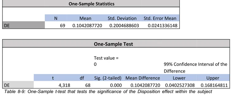
Heukelom (2011) explains how validity originates from psychology as a synonym of the accuracy of a measurement instrument. Validity refers to the integrity of the conclusions that are deducted from a study. Within the area of validity, there are sub-categories that consist of internal validity and _{external validity amongst others. In order to test the accuracy of our} study, we will take a closer look at internal validity and external validity. The internal validity will be tested by using a t-test to see if the DE, which is the difference between PGR and PLR, is significantly different from 0. A result significantly different from 0 would indicate that the participants as a group do not sell gains and losses equally frequently. While a DE that is different from 0 would indicate an imbalance in selling gains and losses, a positive DE would mean gains are sold more frequently compared to losers, and on the contrary, a negative DE

(23)

would mean losses are sold more frequently compared to gains. The two extremes, a value of 1 and -1 would indicate that the participants only sell winners or only losses respectively.

When instead looking at external validity, the question arises if the results will reflect reality well. To start evaluating this question we will have to look at some of the assumptions made. One major assumption is to assume the participants would act in the same way if they would be dealing with their own money instead of fictional money as in the experiment. While we did not have the opportunity to offer monetary compensation, Frydman and Rangel (2014), as well as Wierzbitzki et al. (2019), did. If our results are similar to those of Frydman and Rangel (2014) and Wierzbitzki et al. (2019) one might argue monetary compensation is not essential in affecting the decisions made. Additionally, monetary compensation does not necessarily increase performance according to Gneezy and Rustichini (2000). Moreover, we assume the participants only want to invest in three stocks as well as possessing a maximum of one stock at any given time. Naturally, this does not reflect investor behavior on the actual stock exchange very well. Here lies a trade-off between internal and external validity. The authors deemed it necessary to give up some external validity in order to solidify the internal validity as the DE would be more accurate if it was not possible to sell part of a stock instead of selling 100% of a given stock.

4.2 Methodology

This study will examine the potential existence of the disposition effect for the participants in the selected subject group. If the disposition effect is found, the difference between experienced investors and inexperienced investors will be examined. The disposition effect will be measured by calculating the proportion of gains realized and the proportion of losses realized. The method used which was developed by Odean (1998) is commonly used in papers researching the disposition effect. When the disposition effect has been calculated using this method, the data obtained will be tested using statistical tests. The first one being the one-sample t-test to determine if the whole sample group is exhibiting the disposition effect. If there is an indication of the first statistical test expressing that the whole sample group is displaying signs of the disposition effect. Then this opens up the possibility of testing if there is a difference with regards to experience when testing the disposition effect. In this case, the independent samples t-test will be utilized to see if there is any significant difference while testing this to dissect if the hypothesis selected holds any value. The hypotheses are developed through using existing theory and applying empirical scrutiny on them, Bryman and Bell (2015).

(24)

To perform these tests, primary data will be collected through the experiment that is intended to be used during this study. The experiment consists of a virtual trading game, which is not based on the real-time stock market. By doing this, the setting can be controlled better and first-hand quantitative data can be obtained the instant the subjects finish the experiment to aid the thesis study.

4.3 Research Design

There is a requirement for a consistent method used in order to calculate the disposition effect and attain the desired results. The upcoming section will discuss the quantitative method used for measuring the disposition effect and why it is the most fitting approach to take.

4.3.1 Proportion of Gains Realized / Proportion of Losses Realized

The proportion of gains realized (PGR) and the proportion of losses realized (PLR) that were coined by Terrance Odean in 1998 will be used to calculate the disposition effect in this paper because this approach has been used commonly since it came into prominence. When an investor has stocks in his portfolio that have increased in value above the purchase price and later on are sold, that is a realized gain. On the contrary, if there is a stock in the portfolio that has decreased in value and is currently trading below the purchase price when sold, then this is determined to be a realized loss. However, in cases where the investor decided to not sell the stocks depending on the financial performance, this would be regarded as a paper gain or paper loss instead. Furthermore, there are two formulas used to calculate the PGR and the PLR respectively and these are:

(25)

Since the theory behind the disposition effect states soundly that people are more likely to sell stocks with gains than stocks with losses, it makes it even more obvious to use this measure in order to calculate the disposition effect. Thus, the expectation is that the value of PGR will exceed the value of PLR, which will define the disposition effect (DE) and therefore end up with this final formula:

GR LR E

P − P = D

Hence, if the value of DE is positive i.e, DE larger than zero, then this would indicate a difference between the PGR and the PLR and consequently demonstrates that there is a disposition effect. If the DE is equal to zero then there is no sign of the disposition effect. Lastly, if DE is less than zero then there is a negative relationship and these investors are more likely to realize losses than gains. A limit of 0.05 and -0.05 will be used to determine if there are signs of a positive or negative DE respectively since a value between -0.05 and 0.05 is deemed to be too close to zero to suggest that a DE is apparent.

4.3.2 One Sample T-test

In order to determine if hypothesis I is fulfilled, the one-sample t-test will be used, which is a statistical test that is utilized to examine if the mean of a sample differs from a test value significantly. It is relevant in this study due to the fact that it allows the testing of the mean with regards to previous literature that states that there is a DE if the value is larger than zero by using calculations of PGR and PLR. Therefore, by using the one-sample t-test the value obtained from the sample size could then be examined to determine if it holds any significant value to the study and consequently contributes to the literature regarding this subject. Furthermore, Odean (1998) used a one-sample t-test to test the PGR and PLR while estimating the DE, which is why it is deemed a sensible approach to take.

4.3.3 Independent Samples T-test

If the one-sample t-test proves to be significant then the study will progress to apply an independent samples t-test in order to examine hypothesis II. The independent samples

(26)

t-test is a statistical test that examines the sample means of two independent groups to determine if these means are significantly different. To perform this statistical test, dummy variables will be used for the two different populations that are inexperienced and experienced to determine if hypothesis II can be rejected or not. Also, Wierzbitski et al. (2019) used a two-tailed t-test to test their data, thus solidifying the judgment with regards to what test would be used on the data.

4.3.4 Spearman Correlations

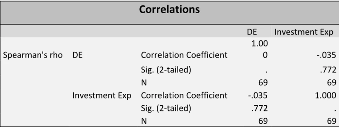
To further test hypothesis II, Spearman correlations will be tested to see if significant correlations exist between the exhibited DE and the self-proclaimed investor experience. Spearman correlation was chosen over Pearson due to the fact that the increase of experience may not show a consistent decrease in DE. The hypothesis assumed that experience and DE would follow a monotonic relationship whereas if experience increases, DE would decrease. While correlation does not equal causation, a strong significant negative correlation between experience and DE will strengthen the hypothesis that experience makes investors less prone to the disposition effect.

4.4 Data

4.4.1 Data collection

The idea behind our data collection has been influenced by Frydman et al. (2014) and Wierzbitski et al. (2019) due to the simplicity of the asset market in their stock games which makes it easy to understand for participants. The programming behind the experiment was provided by Dr. Marc Wierzbitski at the WHU - Otto Beisheim School of Management. The code is adjustable which makes it convenient to alter the program in order to fit the idea for the experiment in this thesis. The program utilized in the experiment was set up by using web technologies such as Javascript, CSS, and HTML. When comparing our version and the one by Wierzbitzki, the biggest difference is the number of rounds played in the game. While Wierzbitski et al. (2019) let the participants play for 100 rounds, due to practical convenience the participants in this study will play for 36 rounds. This was done in order to decrease the amount of time spent due to the fact that they were not provided any monetary compensation for taking part in this experiment and were doing this voluntarily. Furthermore, the decision was taken to lower the number of rounds in comparison to Frydman et al. (2014) and Wierzbitski et al (2019) to maintain the maximum attention span possible of the participants in the experiment while simultaneously having enough rounds to get a dataset

(27)

where a correlation between the decision-making and financial behavior can be determined. According to estimates, reading the instructions and playing 36 rounds with some time to think before making a choice will take between 10 to 15 minutes. Naturally, this results in a trade-off between keeping the participants motivated as the experiment is not as time-consuming but on the other side, the result will be slightly less statistically significant seeing as the data set will be smaller.

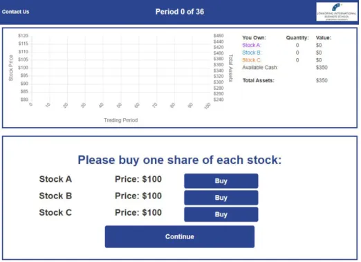
The data collected for this study will be based on a study consisting of 73 participants. The participants are mostly students and faculty members at Jönköping University with a varying degree of experience in finance. All of the participants signed a GDPR consent form prior to participating in the study. In the study, each participant was asked to act as an investor in the stock market with a goal to maximize a given amount of wealth. The stock simulation game used in the study was emailed to the participants. Upon entering the game, each participant is given 350 fictional dollars and three stocks available to buy, stock A, stock B, and stock C. Firstly, each participant is required to buy all three stocks. Secondly, 8 test rounds are being played where the participant can only watch and gain an understanding of how the game works. In other words, they are not allowed to sell the stocks that were purchased in round 0 until they have passed these test rounds. Lastly, in round 9, the participants are allowed to make sell decisions. The participants can trade the stocks for the following 28 rounds before the game is finished and the decisions made are gathered. The experiment could be performed in two(2) ways, i) by receiving an email with a “zip file” and ii) by playing the game locally on the authors’ computer. In the first alternative i) the program was sent through an email with a “zip file” where they had to download it on their computer in order to execute the game. After the game was finished the computer automatically downloaded a “JSON file” with the data from the experiment, which was sent back to us to interpret. The second alternative ii) the experiment was conducted by letting participants play the game locally on the authors’ computer, which accelerated the process since there was no need having to explain how to execute the experiment on the respective person's computer. Moreover, this meant the data was stored instantly on the safe JU-server according to GDPR and there was no need for the participants to send it back through an email, thus limiting data loss.

(28)

Figure 2: A screenshot from the simulation game in period 0.

4.4.2 The Recruitment Process and COVID-19

The original plan for the data collection was to ask students at Jönköping University enrolled in the course “Corporate Finance” to participate in the study. This particular class was chosen due to the fact they would have some prior experience and interest in finance and also computer lab sessions led by a teacher. A few students were able to participate in the study before the virus known as COVID-19 reached Sweden to a larger extent. On the 11th of March 2020, the World Health Organization made the assessment that COVID-19 can be characterized as a pandemic . Due to the pandemic, Jönköping University chose to 3 temporarily move classes from the school to the internet on the 18th of March 2020 . In 4 regard to this, the data collection had to be done through email to willing participants which led to a broader spectrum of participants. This led to participants throughout the country with varying degrees of experience in finance and a broader age-span than if it would have been merely students. Even though recruiting through email proved to be challenging, we managed to collect a total of 73 responses whereas 4 had to be removed due to technical

3_{https://www.who.int/news-room/detail/27-04-2020-who-timeline---covid-19} 4

https://ju.se/om-oss/jonkoping-university/informationsmaterial/uppdaterad-information-med-anledning-av-coronaviruset.html

(29)

difficulties or the data not being up to the required quality, which will be elaborated on in 4.5.1. The data was collected during March 2020.

4.5 Game Structure

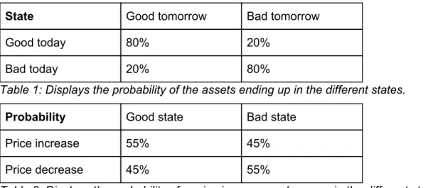
Before the first round, each of the three stocks is given a bad or good state with a probability of 0.5 each. If a stock is in a good state, it has a probability of 0.8 to remain in the good state and a probability of 0.2 to switch to the bad state before the next round. If a stock is in the bad state, it has a probability of 0.8 to remain in the bad state and a probability of 0.2 to switch to the good state. While in the good state, the stock will increase with a probability of 0.55 and decrease with a probability of 0.45. On the contrary, if a stock is in the bad state, it will decrease with a probability of 0.55 and increase with a probability of 0.45. This can be found in the tables below. By using a two-state Markow chain as described above, a momentum strategy will be most beneficial for the investors while exhibiting the disposition effect, i.e. selling winners and keeping losers will lead to inferior returns. More explicitly, a stock that recently decreased in value has a higher probability of being in the bad state and thus more likely to decrease the following round. On the other hand, a stock which recently increased has a higher probability of being in a good state and thus more likely to increase the following round.

State Good tomorrow Bad tomorrow

Good today 80% 20%

Bad today 20% 80%

Table 1: Displays the probability of the assets ending up in the different states.

Probability Good state Bad state

Price increase 55% 45%

Price decrease 45% 55%

Table 2: Displays the probability of a price increase or decrease in the different states.

The price development of the stocks will be displayed with a graph that is continuously updated after each round. The stocks change in value by $5, $10, or $15 with identical probabilities. Whenever the price is about to update there is a price update screen that is displayed for three seconds before the participant can continue to trade the stocks. This mitigates the chance of the participants making impetuous decisions and forces them to review the price update taking place before making a decision regarding their stocks.

(30)

However, when they reach the trading sequence there is no time limit in regards to how long the participants can take to make a trading decision in the experiment. This process gets repeated until the experiment is finished.

4.5.1 Post-experiment survey

After completing the experiment, the subjects are redirected to a short survey. Questions about gender and age are asked in order to determine if the disposition effect is affected by gender or age. To further categorize the subjects, they are asked to estimate their own investment experience on a scale from 1-10. This method was chosen since investment experience is difficult to measure among students and it was decided that it would be beneficial to let the subjects determine their own investment knowledge, which enables the ability to examine if there are any signs of overconfidence in this regard. By drawing a line at the number 5 in investor experience, the subjects will be divided into two groups, one for the experienced investors and one for the inexperienced investors. More concrete, if a participant rated his or her experience 6 or higher, this person was categorized as experienced while a participant who rated his or her experience 5 or lower, this person was categorized as inexperienced. These groups will be used to answer the question if “experience makes you more or less prone to the disposition effect”. By measuring the disposition effect in each group, a comparison between experienced investors and inexperienced investors will be made to see if there is a significant difference. The disposition effect will be measured both at an individual base and aggregated on the whole group.

Since there is no monetary compensation for completing the experiment, one question in the survey is to evaluate the motivation for completing the experiment. Each participant is asked to rate their motivation for participating in the experiment on a scale from 1 to 10. The higher the motivation from the participants, the more trustworthy their results are. Additionally, the participants are asked if they are familiar with either of three terms, The disposition effect, Loss aversion, and/or Prospect theory. This question is asked in order to provide insight into if knowledge about these theories mitigates the effect.

Furthermore, the desire is that the data will be of the highest quality and therefore there was a control question in the survey that asked: “If you have 100€ and you want to invest in a fund with 3% annual interest rate, how much money will you have after 3 years?” The three corresponding alternatives were: “Less than 103”, “Exactly 103”, and “More than 103” and if

(31)

the participants answered “Less than 103” then their data was removed from the DE calculations since it can be assumed that there is a lack of understanding for the experiment, which would lower the credibility of the obtained data. The entire survey is available in the appendices.

4.6 Strengths and Limitations

The limitations of this paper consist of the study being a quantitative research. This makes it easy to find relationships behind different parameters. However, it also makes it more difficult to draw clear conclusions regarding the results obtained in the study. For example, the reasoning behind why men rate their investment experience higher on average than women in our study. Could the reasoning behind this be due to sheer interest in the area or are there other underlying factors that have to be taken into consideration when comparing the genders in this case? This is an area that has not been focused on due to that it is not in the aim of the study. However, this is a dilemma that could be imposed on all parameters, thus making a case for that the study could be enforced even more by combining the study with some qualitative data in order to make it more thorough. Even though it would be interesting to investigate this aspect, it is an area that is outside of the aim of this thesis and therefore less focus was put into this.

Furthermore, the experiment is limited due to the factor that we did not have the possibility of paying our participants for their involvement in the study, which potentially could have an effect on the motivation but is not a given, this is the reason behind the idea of asking for the motivation of the participants while performing the study in the post-experiment survey. This was a contributing factor behind deciding to limit the number of rounds in the experiment, however, the reality is that the results from the experiment would have higher power if the participants played a higher number of rounds since this would reduce the standard error. Moreover, not compensating the participants could also have an effect on the strategy taken by every participant since it is highly difficult to recreate a scenario where the subjects do not feel the pressure of trading with their own money as stated by Gneezy and Rustichini (2000). Furthermore, as mentioned above the recruitment process was affected by COVID-19, which limited the number of participants in the experiment. Lastly, the performances in the experiment could have an effect on the subjects’ rating in the post-experiment survey. However, the thought behind this was to not let the subjects know what was being tested in order to make sure the data retrieved was unbiased.