Estimating traffic demand risk : a multiscale analysis

Estimating Traffic Demand Risk

- A Multiscale Analysis

Niclas A. Krüger – VTI

CTS Working Paper 2012:14

Abstract

This paper proposes a novel method for estimating the traffic demand risk associated with transportation. Using mathematical properties of wavelets, we develop a

statistical measure of traffic demand sensitivity with respect to GDP. This measure can be adapted in a flexible way to capture risk levels relevant for different

investment horizons. We demonstrate the time-scale decomposition of risk with Swedish traffic demand data for 1950-2005. In general, rail transports show a stronger co-movement with GDP than road transports. Moreover, we examine the volatility exhibited by traffic demand. Our findings suggest that rail investments are more risky than road investments. Since the findings can be used for optimal

investment timing and for choice among public investment alternatives, they are deemed important for public policy in general.

Keywords: Traffic demand, GDP growth, Wavelet, Risk, Real Options, Discount rate

JEL Codes: O11, H54, H43

Centre for Transport Studies SE-100 44 Stockholm

Sweden

Estimating Traffic Demand Risk

- A Multiscale Analysis

Niclas A. Krüger a,b,c a

Centre of Transport Studies, Stockholm b

Swedish National Road and Transport Research Institute c

Swedish Business School, Örebro University Phone: +46 70 33 54 599

E-mail: niclas.kruger@vti.se

Abstract: This paper proposes a novel method for estimating the traffic demand risk associated with transportation. Using mathematical properties of wavelets, we develop a statistical measure of traffic demand sensitivity with respect to GDP. This measure can be adapted in a flexible way to capture risk levels relevant for different investment horizons. We demonstrate the time-scale decomposition of risk with Swedish traffic demand data for 1950-2005. In general, rail transports show a stronger co-movement with GDP than road transports. Moreover, we examine the volatility exhibited by traffic demand. Our findings suggest that rail investments are more risky than road investments. Since the findings can be used for optimal investment timing and for choice among public investment alternatives, they are deemed important for public policy in general.

Keywords: Traffic demand, GDP growth, Wavelet, Risk, Real Options, Discount rate

1 Introduction

It has long been well established that there is a link between economic growth and traffic demand. Economic growth has both short-term and long-term effects on traffic demand. Some long-run determinants of increased traffic demand such as improved infrastructure and affordable car technology depend on GDP growth. The short-term effect of economic growth on traffic demand is a different and more complex issue. The question is whether the steady rise in traffic demand is reinforced by short-term economic upturns. Using data from India Ramanathan (2001) shows that transportation and GDP are cointegrated. Tapio (2005) finds that both freight and passenger transports are weakly decoupled from GDP for Sweden, Finland and the UK in the 1990s. Lahiri and Yao (2005) reveal a close connection between the transportation and business sector cycles in the US.

The relationship between economic growth and traffic demand in Sweden was first analyzed in SIKA (2005). The results indicate that the time series of traffic and GDP are not cointegrated and hence that traffic and GDP will not converge to a long-run equilibrium relationship after short-long-run deviations from each other. Therefore, GDP and traffic do not share a stochastic trend in addition to the deterministic trend exhibited by both time series.

The main uncertainty in infrastructure investments is whether future traffic demand is sufficient to cover the costs of the investment. Even if the strong trend of increases in both GDP and traffic leads to a high utilization at some future point of time, a low utilization during the first years will lead to high costs for society because of the foregone yield on capital that could have been used elsewhere. It is therefore important to examine the volatility in traffic demand as a risk measure in infrastructure investments. Since road investments may be seen as real options with regard to

flexibility in time and design, traffic demand variance is an important input for determining the optimal timing and design of infrastructure investments. The higher the volatility, that is, the uncertainty with regard to future traffic demand, the more valuable the option to defer the investment and, more generally, the value of flexibility.

Another aspect of infrastructure investments is that they should promote economic growth. However, if traffic demand decreases during economic downturns, infrastructure investments provide no insurance against short-term shocks, business cycle fluctuations and longer term variations in growth. Hence, it is necessary to explore the cyclical behavior of traffic demand and how strongly traffic demand reacts to economic fluctuations. The beta-value, first proposed in Sharpe (1964), measures the sensitivity of financial asset returns to movements in an appropriate market portfolio derived from financial market equilibrium in the Capital Asset Pricing Model (CAPM). There is no direct equivalent to such a risk measure for infrastructure investments that are not traded on financial markets. However, if we assume that GDP-volatility is an appropriate proxy for the average risk in society, we can construct a beta-estimate for infrastructure investment that is valid as a statistical description of how risky infrastructure investments are relative to movements in GDP. A beta-value that is lower than one implies a low risk investment, since GDP affects the yields from the investment only weakly. A beta-value that is higher than one is considered as risky, since the yields are considerably affected by movements in GDP. Whether the beta value is a relevant measure of risk for infrastructure is questionable. Nonetheless, if we look at infrastructure and other public investments as a portfolio of investments, it becomes clear that this is indeed the case: A public investment portfolio consisting entirely of high beta investments will lead to low societal yields from public

investments during bad times, thus providing no insurance or cushion when it is most needed (and vice versa during good times).

Infrastructure investments are special in that they also have a longer investment horizon compared to other projects. The investment horizon for roads in Sweden used in calculations by Swedish authorities is 40 years and for railroads 60 years. The actual lifespan of roads and railroads probably differs; for example, the average lifetime of road pavements is only 12 years (Haraldsson, 2007). A vast range of papers on financial market risk have examined whether the risk changes with the time scale, for example, daily, monthly and yearly returns (for references, see Gencay et al, 2005). This is of potential importance, since the relevant risk measure used for investing should be related to the investment horizon. However, traditional methods when examining different time scales cannot account for the fact that the scales are not sufficiently independent; that is, information from the daily and monthly returns are incorporated in the series of yearly returns (and vice versa). Gencay et al (2005) therefore propose the use of wavelet analysis for multi-scale risk estimation. With wavelet analysis it is possible to analyze the risks for different time scales separately, and hence for different time horizons that might be relevant to different kinds of investors. Wavelet methods transform a time series into several time series, reflecting properties of the original time series for different time scales. The transformed time series can be added together in order to get the original time series, so that the transformed series essentially contain the same information as the original time series.

The purpose of this paper is to contribute to research in transport economics in two ways. First, by examining long-term traffic demand development by using the

number of registered cars1 in Sweden and other traffic demand measures for the years 1950-2006. Second, the use of wavelet analysis facilitates the analysis of traffic demand volatility and the correlation between traffic demand and economic fluctuations. Wavelets have been used to analyze freight transports in Sweden in Andersson and Elger (2008), but with a different focus compared to this paper.

This paper is structured as follows. Section 2 provides descriptive statistics for the time series used and explains the methods we apply. The results are contained in section 3. Our results show only weak correlations between GDP growth and traffic demand growth in terms of person kilometres on roads. However, the number of registered cars is affected by short-term fluctuations in unemployment. By contrast, freight transportation is sensitive to economic fluctuations. In general, rail transportation is more correlated with GDP than road transportation. These results are used to calculate the level of systematic risk for different road and railway investment horizons. We further analyze the wavelet variance decomposition for traffic demand in order to see how total risk is distributed across time scales. Section 4 applies the empirical results to the investment timing decision and the risk adjusted social discount rate. Section 5 concludes the paper with a discussion on the relevance of our findings for public policy.

2 Data and Method

2.1 Descriptive statistics

Data for the number of registered cars is obtained via Statistics Sweden’s homepage www.scb.se. Table 1 summarizes the descriptive statistics of GDP and traffic growth seen over the entire sample period 1950-2005. The mean growth rate is considerably

1_{For a discussion regarding the relationship between cars and kilometers travelled see section}

higher for traffic demand growth in terms of registered cars than for GDP growth (4.6 % versus 2.3 %) and considerably more volatile in terms of standard deviations (5.6% versus 1.8 %). Unemployment is by far the most volatile variable, mainly due to the sudden and persistent rise in unemployment at the beginning of the 1990s.2

Table 1: Descriptive statistics

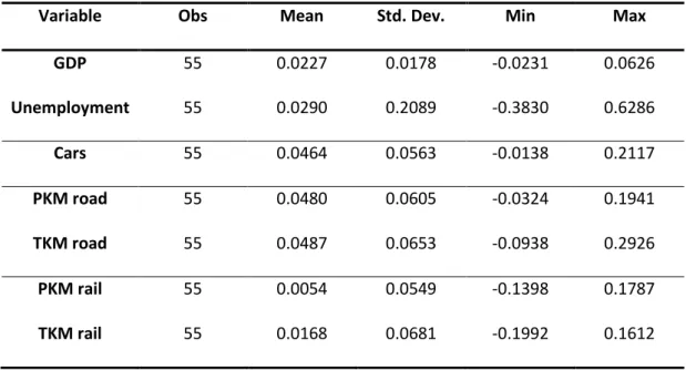
Variable Obs Mean Std. Dev. Min Max

GDP 55 0.0227 0.0178 -0.0231 0.0626 Unemployment 55 0.0290 0.2089 -0.3830 0.6286 Cars 55 0.0464 0.0563 -0.0138 0.2117 PKM road 55 0.0480 0.0605 -0.0324 0.1941 TKM road 55 0.0487 0.0653 -0.0938 0.2926 PKM rail 55 0.0054 0.0549 -0.1398 0.1787 TKM rail 55 0.0168 0.0681 -0.1992 0.1612

Moreover, our analysis uses annual person-kilometer and ton-kilometer data for roads and railroads for the period 1950-2005. Ton-kilometer (TKM) and person-kilometer (PKM) data for road transportation is obtained from the statistics section of the Swedish Institute for Transport and Communications Analysis web-page ( http://www.sika-institute.se). The methods used for constructing these time series are described in SIKA (2004). We can see that traffic growth in terms of both passenger kilometers and transport kilometers is circa 4.8 % per annum with a mean deviation of 6 %. In contrast, rail traffic grows considerably less, by about 0.5 % per year in terms of passenger

2_{The time series of unemployment rates in Sweden was retrieved via ECOWIN for the time}

period 1970-2005 and extended backwards using an unpublished series kindly provided by Olle Krantz.

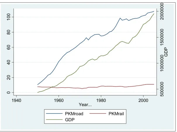
kilometers and 1.7 % in terms of ton kilometers. The standard deviation in the time series of rail traffic is comparable to that of road traffic (5.5 % for passenger kilometers and 6.8 percent for ton kilometers). Figure 1 and Figure 2 visually compare GDP and the traffic demand measures used.

Figure 1: Comparison PKM (billion km) and GDP

5 0 0 0 0 0 1 0 0 0 0 0 0 1 5 0 0 0 0 0 2 0 0 0 0 0 0 G D P 0 2 0 4 0 6 0 8 0 1 0 0 1940 1960 1980 2000 Year... PKMroad PKMrail GDP

Figure 2: Comparison TKM (billion km) and GDP

2.2 Time-scale decomposition of risk

If traffic demand decreases during economic downturns, infrastructure investments provide no insurance against economic downturns. Hence, it is necessary to explore how strongly traffic demand reacts to economic fluctuations. The beta-value, first proposed in Sharpe (1964), measures the sensitivity of financial asset returns to movements in an appropriate market portfolio derived from financial market equilibrium in the Capital Asset Pricing Model (CAPM). There is no direct equivalent to such a risk measure for non-traded infrastructure investments. It is however possible to construct an analogous measure if we assume that GDP-volatility is an appropriate proxy for the average risk in society. It is not a result of market equilibrium, but a statistical description of how risky infrastructure investments are relative to movements in GDP. For example, a beta-value that is lower than one implies a low risk investment,

5 0 0 0 0 0 1 0 0 0 0 0 0 1 5 0 0 0 0 0 2 0 0 0 0 0 0 G D P 0 1 0 2 0 3 0 4 0 1940 1960 1980 2000 Year... TKMroad TKMrail GDP

since a GDP-downturn affects the yields from the investment only weakly. A public investment portfolio consisting entirely of high beta investments will lead to low societal yields from public investments during bad times, thus deepening economic downturns (and vice versa during good times).

The main prediction derived from the CAPM is that the return for holding an asset is related to the riskiness of the asset. Nonetheless, the return demanded and received by investors is only related to the risk that cannot be diversified away through an appropriate investment portfolio. The main conclusion of the CAPM is the so-called security market line, given by:

2 ) , ( ) ( ) ( m m i f m f i r r Cov r r r r E

σ

Where rf is the risk-free return, rm is the return on the market portfolio and σ2m is the variance of the market portfolio. The level of systematic risk is known as the beta-value of the asset i: 2 ) , ( m m i i r r Cov

σ

β

Usually, the beta value is estimated by OLS using the following relationship:

i f m i f i r r r r − )=β ( − )+ε ( (3)

where εi is a white-noise distributed error term. If we assume that the return from infrastructure demand is related to the growth rates of infrastructure usage and that the systematic risk is related to GDP-growth rates, we can state that the infrastructure investor should expect a return proportional to the excess return from societal investments, where the proportionality factor is the beta-value of the infrastructure investment; that is, the sensitivity of traffic demand growth with respect to fluctuations in GDP-growth rates. It is important to bear in mind that the CAPM is derived from rather strong assumptions (and therefore heavily debated) and that it describes

equilibrium in financial markets. Infrastructure investments, on the contrary, are seldom traded in financial markets, with the exception of railroad stocks in the US, for example. Hence, in a positivistic sense, the relationship in Equation (1) is probably incorrect for infrastructure investments. Still, we believe that it has important normative implications for better public investment spending.3

Whereas the level of systematic risk is important for constructing a well-diversified portfolio of public investments, some investment-related decisions are not dependent on the beta-value but on the volatility exhibited by the underlying value-driving process. An extensive discussion of real option valuation is beyond the scope of this paper, but an important real option related to infrastructure is the optimal timing decision. Given that the underlying uncertainties (mainly traffic demand) are stochastic, we want to solve the following problem (see Chapter 5 in Dixit and Pindyck (1994) for details):

( )

[

(

)

]

where F

( )

is the discount rate. The problem we have to solve is to choose an optimal time for the investment in the public project; that is, to pay the amount I for a public project giving the societal net benefits V. As traffic demand evolves stochastically over time, the value V of the project will vary in a likewise fashion. Hence, we will not be able to find an optimal point of time, but a critical value V* determining that it is optimal to invest as

* V

V ≥ . The solution is given by:

3

According to Arrow and Lind (1970), risk should not matter for public investments and decisions should be based on expected net benefits. The assumptions needed to arrive at this conclusion are quite restrictive, so we believe that risk should be taken into consideration.

I b b V 1 * − = (6)

where b is a function of the parameters σ, ρ and δ (δ denotes the expected value growth). Since it can be shown that b>1, the critical value level V* has to be larger than the amount I needed for investment. By differentiating equation (6) partially, we can derive the comparative static properties of the solution. The general implication is that volatility increases the option value of investing since the future becomes more uncertain, leading to a higher threshold value for immediate investment. Hence, traffic demand variance is important for determining the threshold value for optimal investment timing.

Since infrastructure investments usually have time horizons spanning several decades, the question that arises is what time scale we should use to estimate risk. It seems intuitively inappropriate to relate monthly traffic flows to the monthly economic activity index constructed by Statistics Sweden; we expect the sensitivity of traffic demand with respect to longer term variations in GDP to be a better measure. Likewise, estimating volatility with the use of daily traffic flow measurements would probably overstate the relevant risk. We therefore propose risk measurement based on wavelet time-scale decomposition.

We make extensive use of the Haar wavelet as a filter since it is most suitable for the relatively short time series resulting from the short filter length (L=2). The Haar wavelet filter is given by h=

(

)

(

)

=

g . A wavelet filter is defined via certain mathematical properties:

1 0 2 ₌ =

∑

∑

Equation (7) implies a differencing operation (demonstrated below) yielding a series of changes, and equation (8) implies that the transformed series has the same sum of squares as the original series, so that the information content in the transform is the same as the original series.

If we apply the wavelet filter h to a series of growth rates rt we obtain the so-called wavelet coefficients:

1 1 1/ 2 1/ 2

2w_t = r_t − r_t− (9)

It becomes clear that the application of the wavelet filter yields weighted differences of the growth rate series. Applying the scaling filter g we get the so-called scaling coefficients:

1 1 1/ 2 1/ 2

2v_t = r_t + r_t− (10)

In contrast to the wavelet filter, the scaling filter yields weighted sums of pairs of growth rates. Whereas the wavelet coefficients extract high frequency changes, the scaling coefficients produce low frequency changes which could be interpreted as local averages. Using the wavelet filter h and scaling filter g on v1t yields the wavelet coefficients w2t and scaling coefficients v2t, which cover a lower frequency band. This process can be repeated to extract other frequency bands. Denoting the time scale with j we can interpret the wavelet coefficients as the differences of averages over 2j-1 growth rates, and the scaling coefficients as averages of 2j growth rates (Gencay, 2005). For each time scale we can define the wavelet variance as Var(wj) and the wavelet covariance for two times series a and b as Cov(wja, wjb). This property of wavelets allows us to estimate a time scale dependent beta value as a statistical measure of how sensitive traffic demand is with respect to GDP-fluctuations:

(

)

(

)

β

3 Results

3.1 Economic fluctuations and traffic demand

3.1.1 PKM and TKM for road traffic

Growth rates are calculated as the log differences of traffic demand and of real GDP per capita. We decompose the transformed series into their timescale components using the maximum overlap discrete wavelet transform (MODWT). The wavelet filter used in the decomposition is the Haar-filter of length L=2, with periodic boundary conditions.4 The application of the wavelet transform with a number of scales J = 4 produces four sets of wavelets and one set of scaling filter coefficients. Since we use yearly data, scale 1 represents 2-4-year period dynamics, while scales 2, 3, and 4 correspond to 4-8, 8-16 and 16-32-year period dynamics. With wavelet analysis we can disentangle the variance, correlation and cross-correlations on a scale by scale basis and determine which scales contribute to the overall relationship between two series.

Table 2 summarizes the correlation coefficients between GDP-growth and changes in PKM. We cannot find any major correlations between the series with regard to the magnitude of the coefficients and the statistical significance. Deviations from the trend in GDP-growth with various periodicities therefore do not reinforce PKM-growth for the post-war period. We also check whether there are significant correlations among

4

The coefficients generated by MODWT are affected by the boundary condition at the beginning and the end. If the filter is of length L, (2j-1)(L-1) coefficients are affected for scale j, whereas (2j-1)(L-1)-1 beginning and (2j -1)(L-1) ending details and smooth coefficients are affected (Percival and Walden, 2000). For this reason we use the Haar-Wavelet since it has the shortest possible filter length (L=2) and therefore ensures the lowest possible influence from the boundary coefficients.

various leads or lags but the analysis yields no significant results either (the detailed results are not shown here).

Table 3 shows the results for registered cars, where a discernible short-term effect of GDP on registered cars materializes (scale 1). The correlation is weaker when longer time scales are considered.

Table 2: Contemporaneous correlation for person km & GDP

Table 3: Contemporaneous correlation for registered cars & GDP

Table 4: Contemporaneous correlation for ton km & GDP

Scale Correlation 90%-CI

1 0.0822 -0.1773 0.3310 2 -0.1608 -0.5135 0.2383 3 0.1888 -0.4997 0.7310 4 -0.2256 -1.0000 1.0000

Scale Correlation 90%-CI

1 0.3007 0.0487 0.5168

2 0.1566 -0.2425 0.5103

3 0.2072 -0.4851 0.7398

4 0.0555 -1.0000 1.0000

In contrast, we find a significant impact of economic fluctuations on TKM for scale 2 (see Table 4), which represents 4-8-year period dynamics and corresponds to the length of a typical Swedish business cycle. The relationship becomes weaker as the time scale increases.

Next, we examine the structure of the correlation between different modes of transportation on roads and GDP-fluctuations. As Table 5 reveals, no economic or statistically significant relationship can be found; obviously there are factors other than aggregate income that may explain road-PKM fluctuations. These factors seem to affect travel using different road transportation modes in a likewise fashion, since car and bus usage, in particular, are significantly positively correlated (see Table 6).

Table 5: Correlation between GDP and PKM by transport modes on road

Car Bus Motorcycle

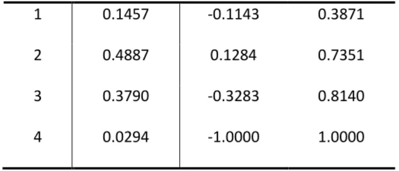
Scale 1 (2-4 years) 0.0518 0.1300 0.0803 Scale 2 (4-8 years) -0.0923 -0.0707 -0.0791 Scale 3 (8-16 years) 0.1291 0.2275 0.1105 Scale 4 (16-32 years) -0.0067 0.1461 -0.2235 1 0.1457 -0.1143 0.3871 2 0.4887 0.1284 0.7351 3 0.3790 -0.3283 0.8140 4 0.0294 -1.0000 1.0000

Table 6: Correlation between PKM by transport modes on road

Car&Motorcycle Car&Bus Motorcycle&Bus

Scale 1 (2-4 years) 0.4806* 0.5240* 0.5772*

Scale 2 (4-8 years) 0.3769* 0.5310* 0.2765

Scale 3 (8-16 years) 0.1923 0.5658 0.0368

Scale 4 (16-32 years) 0.1048 0.7106 -0.2001

3.1.2 PKM and TKM for railroad traffic

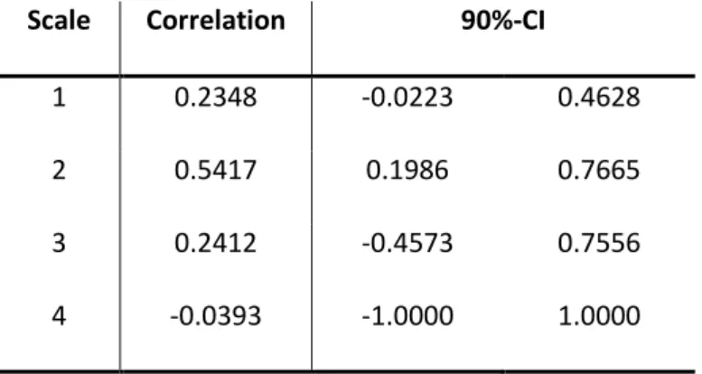
Table 7 summarizes the correlation coefficients between GDP-growth and changes in PKM. In contrast to the results for road traffic, we find a significant correlation between the series with regard to the magnitude of coefficients and statistical significance. Deviations from the trend in GDP-growth therefore reinforce rail-PKM growth for the post-war period.

Table 7: Contemporaneous correlation for person km on rail & GDP

Scale Correlation 90%-CI

1 0.2348 -0.0223 0.4628

2 0.5417 0.1986 0.7665

3 0.2412 -0.4573 0.7556

Moreover, we find a significant impact of economic fluctuations on TKM for scale 1 and scale 2 (see Table 8), which represent short-term shocks and the business cycle, respectively.

Table 8: Contemporaneous correlation for ton km on rail & GDP

Goods transportation as measured by ton-kilometers is positively correlated between road and rail (see Table 9), due to the fact that TKM for both road and rail moves pro-cyclically with GDP. This may be due in part to the fact that road and rail transports are complementary, since goods are often transported by road to the nearest train station. In contrast, road-PKM rises as rail-PKM falls (see Table 10). As aggregate income does not explain fluctuations in PKM-measurements, the factors driving increases in road-PKM seem to decrease rail-road-PKM simultaneously, so that they seem to be substitutes rather than complements.

Table 9: Correlation TKM road and TKM rail

Scale Correlation 90%-CI

1 0.5518 0.3446 0.7077

2 0.5815 0.2537 0.7894

3 0.4871 -0.2047 0.8544

4 0.6301 1.0000 -1. 0000

Scale Correlation 90%-CI

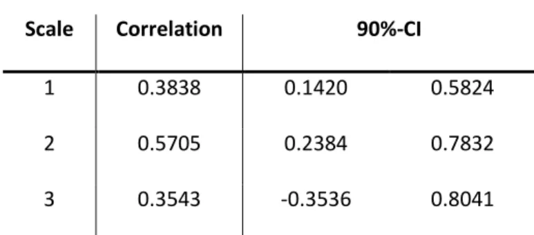
1 0.3838 0.1420 0.5824

2 0.5705 0.2384 0.7832

Table 10: Correlation PKM road and PKM rail

In order to summarize we replicate the analysis performed in this and the preceding section with unemployment data (see Table 11). For rail-TKM the results resemble those using GDP, while the effect of unemployment on rail-PKM is more clear-cut. Considering road transports, the results with regard to registered cars and PKM are similar to the results shown in the previous section, but, in contrast to GDP, unemployment has no statistically significant effect on TKM.

Table 11: Correlation transportation and unemployment

Car PKM road PKM rail TKM road TKM rail

Scale 1 -0.2824* -0.1317 -0.4820** -0.1102 -0.4582**

Scale 2 -0.2351 -0.1417 -0.6348** -0.3560 -0.5099**

Scale 3 -0.1608 -0.2391 -0.3791 -0.0443 -0.0411

Scale 4 0.1490 0.1394 -0.3984 0.3333 -0.2053

4 0.4319 -1.0000 1.0000

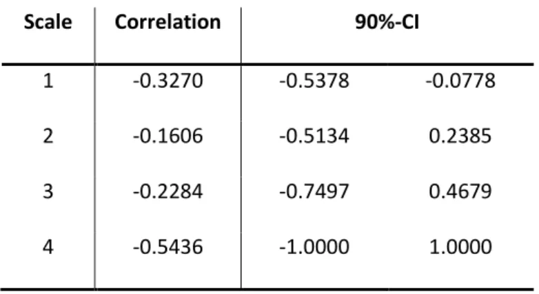
Scale Correlation 90%-CI

1 -0.3270 -0.5378 -0.0778

2 -0.1606 -0.5134 0.2385

3 -0.2284 -0.7497 0.4679

3.2 Time scale decomposition of volatility

The total variance in a time series can be decomposed by means of wavelet analysis of variances across time scales. This property of wavelet decompositions has successfully been used in finance (Gencay et al, 2001) and macroeconomics (Gallegati, 2007).

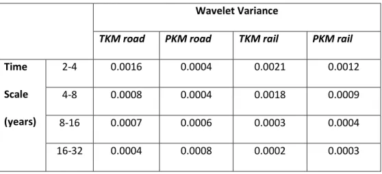
Table 12 illustrates the wavelet-based variance of the traffic demand series used for the different scales. An approximate linear relationship emerges between the wavelet variance and the wavelet scale with the former decreasing as the latter increases, but not in the case of road-PKM.

Table 12: Time scale decomposition of variance

Wavelet Variance

TKM road PKM road TKM rail PKM rail

Time Scale (years) 2-4 0.0016 0.0004 0.0021 0.0012 4-8 0.0008 0.0004 0.0018 0.0009 8-16 0.0007 0.0006 0.0003 0.0004 16-32 0.0004 0.0008 0.0002 0.0003

The analysis of the wavelet variances for ton kilometres shows that volatility declines with the time horizon for TKM. A comparison reveals that PKM-volatility is less than TKM-volatility for the finest scales. Summing the variances and taking the square root show that, in comparison with the standard deviations in Table 1, the total variance in the time series used is, as expected, approximately additively decomposed by wavelet analysis. Small deviations stem from the fact that the standard deviations in table 1 also incorporate the variations caused by shifting means of the series (trend), which are

filtered away in our analysis. The additivity property of variance implies that standard deviations cannot be decomposed across time scales. However, since standard deviations have a simple interpretation, in our case as mean deviations in percentage units, we show the square roots of the variance estimates in Table 13.

Table 13: Square root of wavelet variance

Square Root of Wavelet Variance

TKM road PKM road TKM rail PKM rail

Time Scale (years) 2-4 4.00% 2.00% 4.58% 3.46% 4-8 2.83% 2.00% 4.24% 3.00% 8-6 2.65% 2.45% 1.73% 2.00% 16-32 2.00% 2.83% 1.41% 1.73%

3.3 Time scale decomposition of GDP-sensitivity

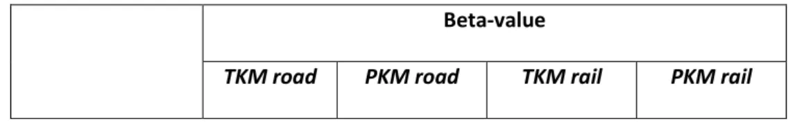
Wavelet analysis makes it possible to decompose the variance and the covariance on a scale by scale basis. Using a measure analogous to the concept of beta-value used in finance (see equation 11, section 2.2), we can estimate the riskiness exhibited by traffic demand for each time scale separately, provided that the non-diversifiable societal risk is measured by fluctuations in GDP. Since the covariance and variance are dependent on the time scale, we also expect the beta-value to be different across time scales. Table 14 summarizes the estimated beta-values.

Table 14: GDP-sensitivity over different time scales

Beta-value

Time Scale (years) 2-4 0.77 0.12 2.70 0.86 4-8 1.25 -0.19 2.49 1.63 8-16 1.36 0.42 1.22 0.66 16-32 0.82 -0.03 1.65 -0.12

Looking at the road-PKM for the post-war period, we do not see any major impact of GDP on time scales, except for dynamics with a period of 8-16 years. In comparison, rail-PKM is much more prone to be affected by GDP-fluctuations.

A priori, we expect ton kilometres to be more dependent on GDP-fluctuations. Our results confirm this hypothesis for both road and railway transports. Most importantly, regardless if we measure transport by ton-kilometres or passenger-kilometres, we find that railroad investments are more risky than road investments. One notable exception is dynamics with a period of 8-16 years, where the beta-values for rail transports and road transports are quite close to each other.

4 Applications

In the following we briefly demonstrate the use of the results presented in the previous section for infrastructure investment planning. We focus here on two important issues: (i) the timing of infrastructure investments and (ii) the risk adjusted social discount rate.

(i) Timing of road and rail investments: The results from the previous section have important implications for public policy concerning the timing of road and rail investments, the choice between road and rail investments and the choice between goods transport investments and passenger transport investments. The measurement of traffic demand variance is a central input for investment timing. The additivity property of variances in wavelet time-scale decomposition allows us to filter out certain parts of

volatility, which are irrelevant to the investment decision and therefore should not affect investment timing. In the context of real option valuation it seems reasonable that long-term variations should not matter if the lifetime of the option is limited. If we assume that variations with a periodicity longer than 16 years are irrelevant for real option pricing, we can recalculate the volatility measure using scales 1-3 only. For the filtered series we find that the standard deviation for road-PKM is considerably lower than for rail-PKM (3.7 % for road-PKM compared to 5 % for rail-PKM), which is in contrast to the raw data (6 % for road-PKM compared to 5.5 % for rail-PKM). Hence, it seems that road traffic follows a relatively steady growth path, where the volatility arising from strong growth behaviour contaminates the volatility measure calculated on raw data. Our results therefore suggest, ceteris paribus, a higher threshold for rail investments than for road investments. Using equation (6),5 we find that the differences in volatility suggests that benefits should be 1.32 times higher than the costs for triggering immediate investments related to road PKM. This factor should be 1.37 for investments related to PKM train (that is, 7.8 percent higher). The threshold for immediate investment is even higher for TKM-related investments: 1.43 for TKM-train compared to 1.39 for TKM-road. Hence, since traffic demand is stochastic, the net-present-value rule is incorrect and the investment rule should be differentiated with regard to the riskiness in different types of traffic demand.

(ii) Social discount rate for road and rail investments: The results can be used to determine an adequate social discount rate for public infrastructure investments. If we accept the social discount rate proposed by the European Commission (2006) for public investments (5%) as a proxy for the average social opportunity cost of capital for public investments and assume a risk-free real interest rate in Sweden to be 3 %, we may use

5

β=0.5-α/σ2+(( α/σ2-0.5)2+2ρ/σ2)0.5, where α is expected value growth of the investment and ρ is the discount rate. In order to isolate the effect of volatility, we assume α=0.02 and ρ=0.05.

the formula: ρ=rf+β(SOCC- rf), where ρ is the risk-adjusted discount rate, rf is the risk-free interest rate and SOCC is the social opportunity cost of capital for public investments. We assume here that the beta of an average public investment is equal to one (for example, demand for higher education increases during economic downturns) and that the relevant beta is measured on scale 2 (business cycle dynamics). We can conclude that future net benefits from investments directed towards rail passengers should be discounted by 6.2 % compared to 2.6 % for car passengers. However, the determination of an appropriate discount rate for public investments is a long-debated subject and beyond the scope of this paper; nevertheless, this example demonstrates the potential use of our approach.

5 Conclusions

This paper applies wavelet analysis to investigate the relationship between traffic demand and economic activity over different time scales. Through a scale by scale decomposition of the variance of the series and the correlation and cross-correlation for bivariate time series, we try to shed some light on the scaling properties of changes in traffic demand and GDP growth rates, and on their relationship at different time horizons.

This paper has arrived at several insights into the properties of traffic demand and risk associated with infrastructure investments. In the following we briefly summarize the main results:

- Passenger road-kilometres are only weakly correlated with GDP.

- Traffic demand variance decreases with the length of the time span considered. Volatility is therefore mainly a short-term phenomenon (2-4 years, see below for a discussion of the implications).

- The pattern is repeated for the GDP-sensitivity of traffic demand: We find strong pro-cyclical movements in traffic demand, especially for short-term economic shocks and business cycle dynamics, with the noteworthy exception of road-PKM. We find the least risk for the time scale covering periodicities of 8-16 years. - For most time scales, railroad investments are more risky in terms of

GDP-sensitivity compared to road investments.

- Investments that focus on goods transport (as measured by ton-kilometres) are more risky than investments in passenger transports.

The results have important implications for public policy concerning the timing of road and rail investments, the choice between road and rail investments and the choice between goods transport investments and passenger transport investments. Risk in transportation investments is also important for public tender in that it might favour big companies (because of their ability to diversify risk), for financing decisions (private vs. public) and risk sharing conditions in public-private partnerships.

In this paper, we demonstrate the usefulness of the results by calculating the implications on investment timing and for determining an appropriate discount rate. Since the relevant risk measure should be related to investment time horizon, we believe that time scale decomposition provide an important contribution for calculating risk. Our findings indicate both a higher social discount rate and a higher hurdle rate (the factor by what benefits should exceed costs) for tonne-km related investments than to passenger-km related km. The same is true for rail-investments compared to road-investments.

It has been argued in Andersson and Elger (2007) that the procyclical character of transport demand will lead to bottlenecks in the transport system during phases with high economic activity. Even if this is true in a physical sense, a portfolio perspective

gives a somewhat different picture: Only investing in projects with high sensitivity with regard to GDP will lead to a more volatile outcome. It would be like lowering interest rates during economic booms when credit demand is high and hence credit is relatively scarce. Yet no modern day central banker thinks that this is a good idea and instead smoothes credit demand over time. Moreover, during off-peak periods capital would be tied up in unused capacity. Our analysis show that even in a more narrow perspective, considering only transport projects, the differences in volatility and GDP-sensitivity in transport demand makes it important to incorporate traffic demand risk in societal cost-benefit analysis of transportation projects.

References

Andersson, F. N. G. and Elger, T., (2007), Freight Transportation Activity, Business Cycles and Trend Growth, Working Paper No. 2007:15, Department of Economics, Lund University

Arrow, K. J. and Lind, R. C., (1970), Uncertainty and the Evaluation of Public Investment Decisions, American Economic Review, 60, 364-78.

European Commission, (2006), The New Programming Period 2007-2013: Guidance on the Methodology for Carrying out Cost-Benefit Analysis, Working Document No. 4

Gallegati, Marco and Gallegati, Mauro, (2007), Wavelet Variance Analysis of Output in G-7 Countries, Studies in Nonlinear Dynamics and Econometrics, 11, No. 3

Gencay R., Selcuk F. and B. Whitcher, (2001), Scaling properties of foreign exchange volatility, Physica A, 289, 249-266.

Gencay, R., Selcuk, F. and Whitcher B., (2002), An Introduction to Wavelets and Other Filtering Methods in Finance and Economics, San Diego Academic Press

Gencay, R., Selcuk, F. and Whitcher B., (2003), Systematic Risk and Timescales, Quantitative Finance, 3, 108-116

Gencay R., Selcuk F. and B. Whitcher, (2005), Multiscale systematic risk, Journal of International Money and Finance, 289, 249-266.

Haraldsson, M., (2007), Essays on Transport Economics, Department of Economics, Uppsala University, Economic Studies 104.

Lahiri, K. and Yao, V.W., (2006), Economic indicators for the US transportation sector, Transportation Research Part A, 40, 872-887.

Walden, T. A. and Percival, P. D., (2000), Wavelet Methods for Times Series Analysis, Cambridge University Press.

Ramanathan, R., (2001), The long-run behaviour of transport performance in India: a cointegration approach, Transport Research Part A, 35, 309-320.

Sharpe, W., (1964). Capital asset prices: a theory of market equilibrium under conditions of risk, Journal of Finance, 19, 425–442.

Tapio, P., (2005), Towards a theory of decoupling: degrees of decoupling in the EU and the case of road traffic in Finland between 1970 and 2001, Transport Policy, 12, 137-151.

SIKA, (2004), Transportarbetets utveckling, SIKA PM 2004:7.

SIKA, (2005), Den ekonomiska utvecklingens påverkan på transporterna, SIKA PM 2005:15.