V¨
aster˚
as, Sweden
Thesis for the Degree of Master of Science in Computer Science
-15.0 credits
EVENT BASED PREDICTIVE
FAILURE DATA ANALYSIS OF
RAILWAY OPERATIONAL DATA
Jan Hric
jhc19001@student.mdh.se
Examiner: Ning Xiong
M¨
alardalen University, V¨
aster˚
as, Sweden
Supervisors: Wasif Afzal
M¨
alardalen University, V¨
aster˚
as, Sweden
Company supervisor: Amel Muftic
Addiva, V¨
aster˚
as, Sweden
Abstract
Predictive maintenance plays a major role in operational cost reduction in several industries and the railway industry is no exception. Predictive maintenance relies on real time data to predict and diagnose technical failures. Sensor data is usually utilized for this purpose, however it might not always be available. Events data are a potential substitute as a source of information which could be used to diagnose and predict failures. This thesis investigates the use of events data in the railway industry for failure diagnosis and prediction. The proposed approach turns this problem into a sequence classification task, where the data is transformed into a set of sequences which are used to train the machine learning algorithm. Long Short-Term Memory neural network is used as it has been successfully used in the past for sequence classification tasks. The prediction model is able to achieve high training accuracy, but it is at the moment unable to generalize the patterns and apply them on new sets of data. At the end of the thesis, the approach is evaluated and future steps are proposed to improve failure diagnosis and prediction.
Acknowledgements
I would like to thank my supervisor Wasif Afzal for his support and guidance throughout the
thesis. Likewise I would like to thank Amel Muftic and Bj¨orn Laurell, employees of the company
Table of Contents
1. Introduction 1
1.1. Problem Formulation . . . 1
2. Background 2 2.1. Predictive and condition-based maintenance . . . 2
2.2. Train events . . . 2
2.3. Machine learning . . . 2
2.3..1 Neural networks . . . 2
2.3..2 Recurrent and long short-term memory networks . . . 2
3. Related Work 4 4. Method 6 5. Data Structure 7 5.1. Train type . . . 7
5.2. Period length . . . 7
5.3. Time frame length . . . 7
5.4. Period labeling . . . 9
5.5. Failure type . . . 9
6. Data Preprocessing 10 6.1. Period and time frame length . . . 10
6.2. Labeling and class balancing . . . 10
7. Results 12 7.1. Machine learning algorithm used . . . 12
7.1..1 Prediction model architecture . . . 12
7.2. Failure diagnosis . . . 13
7.2..1 Further experimentation . . . 13
7.3. Failure prediction . . . 16
8. Discussion 20 8.1. Answers to research questions . . . 20
8.2. Threats to validity . . . 20
8.3. Future work . . . 21
9. Conclusions 22
References 24
1.
Introduction
The railway industry still plays a very important role in both passenger and cargo transportation and as in other areas, data analysis is being used to improve efficiency of railway operations and
reduce operational costs [1]. One way to reduce the costs is by using predictive maintenance.
Predictive maintenance is based on predicting failures and scheduling necessary maintenance to prevent them, as preventing a failure is almost always less costly than dealing with its consequences when it actually occurs.
Data used for such analysis and predictions can be classified into 2 groups with respect to the type of the data used:
1. Continuously recorded sensor data 2. Event based data
In case of continuously recorded sensor data, various values, such as voltage, temperature or vibrations, are recorded at all times and failures are predicted by comparing values preceding the occurrence of a failure with data collected in times during which no failures occurred. Event based prediction, on the other hand, attempts to predict failures based on events that are recorded on an irregular basis. Such events can include regular operations (such as opening of doors) or events that usually do not or should not occur (such as decreased voltage in battery). In both cases, failures are usually predicted using various machine learning algorithms.
1.1.
Problem Formulation
The focus of this thesis is on evaluating the data in order to define the steps which need to be taken in order to allow predictive data analysis in the future or, if the data is sufficient, try to apply predictive analysis on the existing data to see if any failures can be predicted. Specifically, the thesis attempts to answer the following questions:
1. What are the most important factors in the data that are currently being collected with respect to predictive data analysis?
2. How do the data need to be processed in order to be used for machine learning algorithms? 3. Why are the currently collected data unsuitable for predictive analysis and what would need
to change in terms of data collection in order to allow predictive analysis in the future? 4. What is the most suitable machine learning algorithm for failure prediction based on events
data?
The work was done in cooperation with the company Addiva [2], which provided real life data
collected from various parts of train vehicles. The data consists of events that happened during the train operation and sensor values, which were recorded at the time a particular event occurred.
2.
Background
2.1.
Predictive and condition-based maintenance
Predictive maintenance is the process of collecting real life operational data, analyzing them in order to predict future failures and then planning maintenance accordingly to prevent the failures from happening. Condition-based maintenance is an extension of predictive maintenance, during which data from sensors is being analyzed in real time and alarms are triggered if the algorithm
predicts an upcoming failure [3]. Both types of maintenance aim to achieve higher up-time and
more efficient and less costly maintenance.
2.2.
Train events
There are various events that can occur on a train and which are automatically recorded by programmable logic controllers (PLCs). PLCs are small units placed in every part of a train, from which data is collected. In our case, the events recorded fall into 4 different categories:
1. Critical events, of which the driver is notified and is required to take an immediate action. 2. Events, of which the driver is notified, but no action is immediately required.
3. Maintenance related events, of which driver is not notified at all, but which are used for maintenance purposes.
4. Common informative events, which can be used for failure diagnosis, but which in themselves do not signal anything unusual or undesired.
This type of categorization is commonly used by railway companies and it may differ in the number of categories and description of the categories, but the existing system, overall, is very similar. Whenever an event occurs, it is recorded in the database. For each event occurrence, date, time, train and event type is recorded.
2.3.
Machine learning
The process, during which algorithms are trained using sample data in order to discover patterns and apply them to another sample is called machine learning. The important aspect of machine learning is that the algorithms are not explicitly told on how to find the patterns or make the
decisions, they are only given the data [4]. There are many machine learning algorithms, which
differ in their performance, sensitivity to outliers, ability to tune the algorithms by modifying the input parameters and the option of seeing details on how the input data affect algorithm’s decisions. For this thesis, neural networks (NN) were chosen as the most suitable machine learning algorithm.
2.3..1 Neural networks
The name neural networks comes from the property of these machine learning algorithms, that the input data go through a network of neurons, which are mapped to an output. The model used for prediction is trained using a training data set, which is a set of data for which the output value is already known. While NNs provide accurate prediction models, they can take a long time to train and they behave like black boxes, i.e. it is very difficult to see how the NN classifies the
input values [5]. For the problem presented in this thesis, recurrent neural networks (RNN) were
selected, as they the input data set was transformed to a set of sequences and thus the problem became a binary sequence classification task, for which RNNs are very well suited.
2.3..2 Recurrent and long short-term memory networks
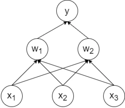
While simple NNs are good at finding patterns among several input parameters, they are unable to capture temporal patterns in the data. In Figure 1 we can see an example of a simple neural network, which takes three different parameters as the input xn, passes them to a hidden layer of
two nodes wn and outputs a single value y. However, if the data is in the shape of a sequence of
values, then we can expect that neighbouring values in the sequence affect each other and simple NNs are unable to capture this behaviour; if we change the order of input nodes, the results will not change, as simple NNs do no take the order of input values into consideration.
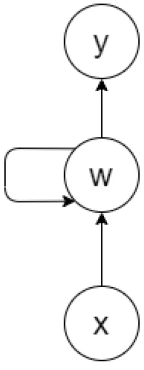
RNNs address this problem by introducing a hidden state, which is used along with the regular weights and which changes after each step of the training process, which in case of sequential data means that the hidden state is updated after processing each value in the sequence. A simple model of a recurrent neural network is depicted in Figure 2. The input x, which is a value in a sequence, is passed to the hidden node w which produces an output value y while updating the hidden state and passing the information to itself in order to use it while processing the next value in the sequence. Even though RNNs can use this technique to capture the relationship between individual values in time, they tend to take into account only the recent values and are therefore
unable to capture patterns in long sequences of data [6]. Long shot-term memory (LSTM) networks
address this problem by introducing gates, which control how the state is updated by individual
input values [7]. The gates can control how much the state should be updated by the individual
inputs and thus allow information to be carried over even in long sequences of data, which is an improvement compared to RNNs, where the state is updated after processing each input value and thus information acquired from values at the beginning of a sequence fail to be carried over to the end of the sequence, as they get overwritten by the more recent values.
Figure 2: Model of a RNN
3.
Related Work
Related work was searched using online academic database Scopus [8]. The database was searched
in two stages; in the first stage, papers focusing in general on predictive maintenance for the railway industry in the area of computer science were searched. This led to finding mostly papers oriented on sensor based prediction models. In the second stage, the aim was to find papers dealing specifically with event based predictions.
Sensor data based prediction has been studied in numerous papers, including [9,10,11], which
studied application of data analysis in the automotive industry or [12, 13], which investigated
failure prediction for tracks equipment. On the other hand, event based prediction is much less popular. This could be caused by two factors. The first one is a considerable disadvantage of event based prediction: the discontinuity of the data stream; the data is recorded neither continuously nor on a regular basis, which makes any kind of prediction more difficult, since vital pieces of information might be missing. The other reason is that in many cases, there are no events to begin with, therefore event related data simply do not exist.
Some work has however been done in this area. Fink et al. [14] conducted a case study on
op-erational disruptions prediction due to malfunctions of the tilting system based on events collected from a train fleet consisting of 52 trains over a period of ten months. The predictive analysis was done using a combination of conditional restricted Boltzmann machines (CRBM) and echo state networks (ESN). The problem was simplified to make up for the quality of the available data; the authors tried to predict whether one or more disruptions would occur in a 6 hour time period or not and achieved very promising results - 98% of all disruptions were correctly predicted in the studied data set.
Another case study was conducted in 2014 by Fink et al. [15]. In this paper, event based
prediction was conducted using Extreme Learning Machines (ELM). The authors present several advantages over other algorithms. The analyzed data set seems to be identical to [14] - this data set also consisted of events recorded on a train fleet consisting of 52 trains over ten months. The goal was to predict failures which would occur in the next seven days, this way the problem could be turned into a binary classification task - either a failure would occur within the next seven days or it would not. In this case, the achieved accuracy was approximately 98%, which is a good result, however it is important to keep in mind that the precision of the failure prediction time was rather low.
Both papers conducted a study closely related to the work done in this thesis, however, in both cases only a single component of the train was studied, while the goal of this thesis is to apply a more general approach and try to predict failures for a whole system or subsystem of a train. Also, contrary to these papers, this thesis focuses on investigating the use of train events data by applying a well known neural network architecture, rather than investigating a new one.
4.
Method
In order to propose the most suitable techniques, a case study was conducted. The main focus was on trying to apply one or more machine learning algorithms on real-life data to provide examples of techniques which could be used by other researchers or railway companies attempting to perform predictive analysis on their data.
In the first phase, the data was analyzed to determine the steps that needed to be taken to transform the data set into a format that can be further used for various machine learning algorithms. It was also necessary to identify which factors would be most relevant for predictive analysis. As part of this phase, a literature review was done to aid the decision making for the proper course of action in the following phases.
After that, the data was preprocessed to create inputs which could be used to train machine learning algorithms, to see if predictive analysis is possible with the currently available data. After reviewing the existing literature, RNNs were selected as the most suitable option and the preprocessed data were then used to train the algorithm to both diagnose and predict failures and a small experiment was conducted using different configurations of the prediction model to achieve the best results.
Based on the results from training the algorithm and applying it on a validation data set, a qualitative analysis of the data was conducted, as the the prediction model showed very poor ability to generalize patterns from the input data and apply them on new data sets. Shortcomings in the present data collection and data structure were pointed out and future steps were proposed to address them and allow predictive analysis in the future. As part of the discussion, future work which could be done with the current data set was also proposed.
5.
Data Structure
The data used in this thesis consist of events recorded on an irregular basis and failures reported over a period of two years on a fleet of 141 cargo trains. The recorded events amount to a total 9,700,000 and the number of failures was 527 in total. The train fleet consists of two distinct types of trains: electric and diesel. This is an important distinction, as each type of train has fundamentally different structure and particular events happen exclusively on only one of these two types, even though they are recorded and stored in the same database. The distribution of the events with respect to train type is uneven; 68% of all events happened on the electric trains, despite the fact that they make 56% of the fleet. The electric trains also consist of a wider variety of event types, 469 in total, while only 269 different types of events can be found on their diesel counterparts.
Failures were recorded manually in the form of a hand written failure report containing de-scription of the failure, date and time when the failure was recorded and a unique identifier of the train. Categorization of the reports was conducted retrospectively by a different person. The reports were divided by the train part that was affected, however each failure type potentially covered various failures that happened on that particular train part. Furthermore, not all reports were records of a failure, some of them were only records of a suspected failure, which may or may not have occurred. This is a significant deficiency in the data, however the analysis was done with the assumption that majority of the recorded failures were actual failures and not just suspected failures.
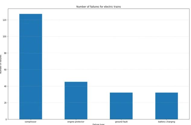
The distribution of failures is proportional to the distribution of train types; 55% of recorded failures occured on electric trains, even though it is important to keep in mind that these are failures that were reported, the actual number of failures might be higher for both types of trains. The failures consist of 5 distinct types with respect to which part of the train was affected. The distribution of failures for both train types can be seen in Figure 3 and Figure 4. Since most failures had a very low number of occurrences, especially after splitting the failures into two groups depending on the train type, the analysis was conducted only for the two most frequent types of failure, that is failures that affected either the train compressor or pantograph (this type of failure occurs only on electric trains, as diesel trains do not have a pantograph), which had an occurrence rate of over fifty instances during the given time period.
There were several parameters of the data, which had to be considered before the preprocessing phase.
5.1.
Train type
There were two distinct groups of events, depending on what type of train they occurred on; electric or diesel. Events recorded on these two types were treated as two separate sets of data, because each event happens exclusively on one type of train.
5.2.
Period length
Each input for the machine learning algorithms was a time period, which either preceded (in case of failure prediction) or both preceded and followed (in case of failure diagnosis) a failure. The length of a period was time, during which events might have had an impact on or might have been used to predict the occurrence of the failure. For example, if we say set the period length to ten days, we are assuming that events happening more than ten days before a failure have no relation to the failure.
5.3.
Time frame length
Each period was divided into individual time frames, for which event occurrences are counted. This parameter influences accuracy and generalization ability of the machine learning algorithm. If we make the length too short, the algorithm might be able to predict failures more accurately, however it will be prone to over-fitting; instead of learning the general pattern leading to a failure, the algorithm will simply remember the individual inputs which led to a failure. On the other hand,
Figure 3: Number of failures for diesel trains
Figure 4: Number of failures for electric trains
if we make the time frame too long, essential information might be lost, making the algorithm unable to learn.
5.4.
Period labeling
Periods are always labeled as either 1 (failure occurred) or 0 (no failure occurred), however we have to choose how the periods are labeled. If we are trying to predict failures, we would label a period as 1 if a failure happened after the end of the period, while in case of failure diagnosis, we would be looking at the impact a failure might have on event occurrences both preceding and following the failure and thus a period would be labeled as 1 if the failure occurred at the end of the period. We also have to be careful with how we choose periods labeled as 0. It is not necessarily true that any period can be labeled as either one or the other. If a failure occurs in the middle of a period, it would not be labeled as 1 in either case, yet the data might contain some patterns related to both failure diagnosis and failure prediction, and thus confuse the algorithm during the training process. It is therefore safer not to include (at least in the initial phases) such periods in the learning process at all.
5.5.
Failure type
Data on five different failure types were available, however not all failure types had a sufficient number of instances to be used in this study, therefore only the two most common failure types were considered: pantograph and compressor failures.
6.
Data Preprocessing
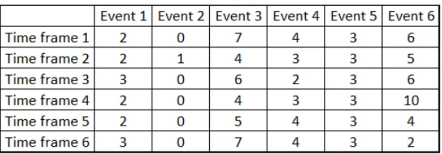
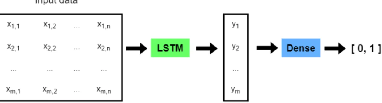
In the first phase, the data were preprocessed into a format that could be used for machine learning algorithms. To generate the individual inputs for machine learning algorithms, the data set was first split into two halves, depending on which type of train (diesel or electric) the events occurred on. Then the events were grouped by the individual trains and time frames during which they occurred, so that each data point had two dimensions; time frame and number of occurrences of a particular event during that time frame; an example of an input value is shown in Figure 5 (each cell represents the number of event instances that were recorded in the given time frame for a specific event). Each individual input value was a time period in the two year range for one train. Transforming the data into this format turned this data analysis problem into a binary sequence classification problem, as each input consisted of sequences (columns in Figure 5), whose number was equal to the number of unique events and the length of each sequence was equal to the amount of time frames (rows in Figure 5) within a period.
Figure 5: Format of the input data, each cell number represents number of occurrences of an event during a time frame
Furthermore, each input was normalized, so that values representing the number of event occurrences were in the range [0, 1], where 0 represents the lowest and 1 represents the highest number of event occurrences during an individual time frame. The normalized values were stored as a 16 bit float number, as this was enough to maintain sufficient precision while reducing the size of the data set and thus memory required for processing.
6.1.
Period and time frame length
The first challenging task was to choose the length of period and time frame. As there was little technical knowledge available, on which the values could be based, period length of four weeks
proposed in [15] was used as the starting value, as the authors dealt with a very similar data
set and were able to achieve positive results. As the nature of this thesis is exploratory, period length of two weeks was added. The motivation for this was to find out how much information is necessary for the machine learning algorithms to learn.
The shortest possible length of individual time frames within a period was one hour. This value was considered to be too short, as it would introduce the risk of over fitting the algorithm to the training data set or producing too granular inputs, from which the algorithm would not be able to learn, given the small amount of failures. Therefore the initial time frame length was set to four hours, which on one hand led to a loss of information, but one the other hand reduced the risk of over fitting and also made the data less granular, which could potentially help the algorithm learn more general patterns. To further explore how granular the data needs to be for the algorithm to learn while avoiding over fitting, time frame lengths of eight and twelve hours were further chosen for experimentation.
6.2.
Labeling and class balancing
To produce inputs labeled 0 (i.e. no failure occurred), the time period was shifted by one week over the two year range for each train to create individual inputs, similarly to [15], excluding periods
during which a failure occurred. For example the first period consisted of events which occurred between January 1, 2018 and January 28, 2018, the next period consisted of events which occurred between January 8, 2018 and January February 4, 2018 etc. until the end of the year 2019. This approach produced an increased number of inputs at the cost of introducing some overlap between individual inputs.
The approach for creating inputs labeled 1 was different, as the classes in the data set are significantly out of balance (less then 1% of all inputs were labeled as 1). Using the same ap-proach as for inputs labeled 0 would create a significantly lower number of inputs labeled as 1 and furthermore, we would not be able to precisely choose the position of the failure within a period. Therefore periods labeled as 1 were generated separately for each failure instance. Most failures are reported within 24 hours of the failure occurrence and nearly all failures are reported no more than 48 hours after the occurrence. To take this into account, the time of failure occurrence was set to midnight the day before the failure was reported, for example if a failure was reported on July 22 at 7:00 p.m., the time of occurrence would be set to July 21 0:00 a.m).
To increase the number of inputs labeled as 1, a variation of oversampling technique called
Synthetic Minority Oversampling Technique (SMOTE) [16] was used. This technique addresses
the class imbalance by synthetically creating new inputs similar to the existing data for the under-balanced class. In this thesis, extra inputs were generated by slightly changing the position of the failure within a period, rather than modifying the number of event occurrences, which would be the usual approach. A period was labeled as 1 if a failure occurred in the last four days of the period and a period was generated for every possible time frame, during which the failure could have occurred. As a result, if the length of the time frame was four hours, each failure would be used to generate 24 inputs, since 6 inputs would be generated for each of the last four days of the period. Although this approach increased the number of inputs labeled as 1, the data set was still significantly out of balance. To further balance the data set, the existing inputs were replicated to achieve desired class balance(at least between 40% - 50% of periods were labeled as 1).
In case of failure prediction, events preceding the failure occurrence by at least two days would be used to create the period. In case of failure diagnosis, failures both preceding and following a failure occurrence would be used. Specifically, a period would be labeled as 1 if the failure occurred in the last four or eight days of the period. Two different values were used to investigate if increasing the amount of events data following the occurrence of a failure would have an impact on the algorithm accuracy or not.
7.
Results
7.1.
Machine learning algorithm used
LSTM networks were chosen as the most appropriate algorithm for this problem, as they have been successfully used for sequence classification tasks by several researchers in the past [17, 18, 19]. LSTM networks are an implementation of RNNs. RNN architecture is designed to capture patterns in temporal sequences and the LSTM implementation further addresses the problem of vanishing gradient, which allows the network to perform better on long sequences of data than regular RNN. These properties make them an ideal candidate for this study, because the input data consists of sequences of values (which represent event occurrences) recorded over a certain period of time and our goal is to find a machine learning algorithm that will capture the temporal patterns in the data and use them to classify the whole sequence, or more precisely, set of sequences (each event type is represented by one sequence).
7.1..1 Prediction model architecture
The data analysis and NNs were both implemented using the programming language Python [20]
and a Python library called Keras [21]. The library provides high level interface and implements
many types of NNs architectures, which allows the user to focus on the application of NNs, rather than their implementation. The architecture of the prediction model consisted of two NN layers. The first layer was an LSTM layer, which transformed each sequence into a single output value. The LSTM layer consisted of one layer of hidden nodes, whose number was equivalent to the number of events, which depends on the train type; 469 different events can happen on electric trains, therefore the input data would consist of 469 sequences and hence the number of hidden nodes in the LSTM layer would be equal to 469, while in case of diesel trains the number of events and hidden nodes would be 261. The second layer was a dense layer connecting all outputs values of the previous layer and producing one output value in the range [0,1]. This layer consisted of the same number of hidden nodes as the LSTM layer. While the number of nodes in this layer should perhaps be lower in order to allow better generalization ability of the model, in this case it was considered better to start with this amount to see if the model would be able to achieve at least sufficient training accuracy using this configuration. The whole model is graphically depicted in Figure 6. Sigmoid function was used as the activation function in both layers. The output value would then be classified as 0 (no failure occurred) if the final output value was less than 0.5, otherwise it would be classified as 1 (failure occurred). Furthermore, Root Mean Square Propogation (RMSProp) was set as the optimizer for the model. The accuracy of the model would then be evaluated by measuring how many predicted labels matched the actual labels.
Figure 6: Model architecture, where the input data consist of m rows (one for each time frame within a period) and n columns (one for each event)
To test the model for overfitting, cross validation was applied during training. The training data set was split into five separate parts of equal size and 80% of the data set was used for training, while the remaining 20% was used for validation. Class balance was always preserved only for the training part. While splitting the data set, each of the five parts contained 20% of the failure periods, however, over sampling was applied only on the training data set to maintain
class balance and prevent the NN from favoring one class solely on the number of inputs. On the other hand, duplicating inputs for the testing part would not add any value, the output would be the same for all duplicates.
The model was trained over only two epochs. This number might seem low, however we have to take into account that the inputs labeled 1 were generated by first creating slightly different copies of the same failure periods and then over sampling those to bring the class balance closer to being equal for both classes. Therefore during each epoch, the model would be updated several times for each failure. As for inputs labeled 0, since their amount is sufficient and there is overlap between the inputs, the low number of epochs was not considered to be an issue from this perspective either. The Python code used to build the model can be seen in Listing 1.
7.2.
Failure diagnosis
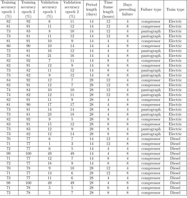
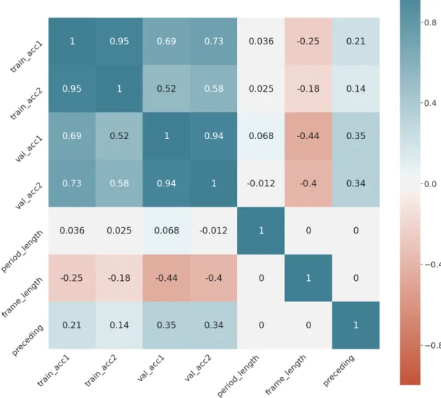
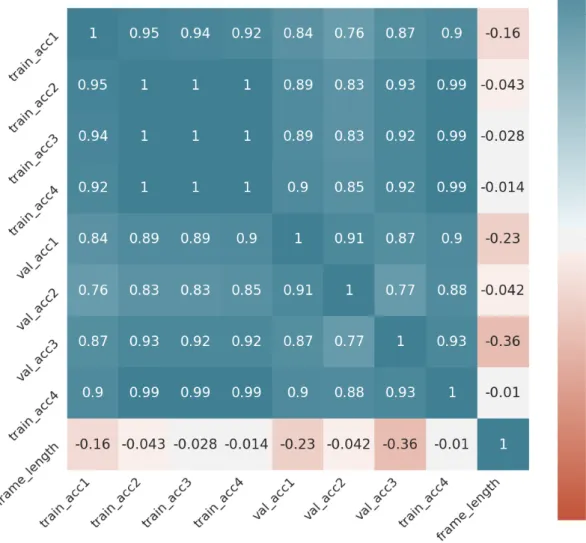
At first, the model was trained for failure diagnosis. The accuracy achieved for each parameter value after training the model with the initial settings can be seen in Table 1. The effect of each parameter on the training accuracy can be seen in the correlation matrix in Figure 7. The matrix shows correlation between each pair of columns in Table 1, for example the fifth column in the first row shows correlation coefficient between training accuracy after one epoch and time frame length. The coefficient between those two is -0.25, which means that the longer the time frame, the lower the accuracy. For any combination of parameter values, the model was able to achieve high accuracy on the training data set, however the accuracy drastically decreases for the validation data set. Upon further examining the prediction, the low validation accuracy turn out to be due to a high number of false positives, which made up majority of the validation data set predictions. The only case where the algorithm validation accuracy got close to the accuracy we would get by randomly guessing the prediction value was for the compressor failure on diesel trains with time frame length of 4 hours. However in this case, the training accuracy after 2 epochs reached 100%, suggesting that the model simply learnt how to predict every single input value in the training data set and thus reaching the extreme case of overfitting, where the model learns perfectly to classify the training data set, but loses ability to classify any new values.
Three explanations were considered for the low validation accuracy of the model: 1. model overfitting
2. absence of any useful patterns in the data 3. incorrect model architecture
The first explanation was considered less likely, as the validation accuracy was low regardless of the training accuracy. Even though we can see in the correlation matrix that the correlation between training accuracy and validation accuracy is around over 0.5, suggesting that the higher the training accuracy, the higher the validation accuracy, the validation accuracy still remained very low (less than 25% in the best case, if we exclude the extreme cases of overfitting mentioned in the previous paragraph). The absence of useful patterns in the data was considered a possible explanation, as there was no previous knowledge about the data which would count as evidence that the information, which could be used for failure diagnosis or prediction, was present in the data. This, however, was the motivation for this study; to find out whether the information in the data was or was not present. To test whether the last explanation was the reason for the low validation accuracy, different model architecture had to be considered and tested.
7.2..1 Further experimentation
Not all combinations of parameter values were used for further experimentation. From looking at the correlation matrix, we can see that period length had no effect on the achieved accuracy, therefore the period length of 28 days was removed and only the period length of 14 days was kept, as this way the amount of data used for training would be reduced without sacrificing model accuracy. Time frame length on the other hand had a negative impact on the model accuracy. This was to be expected, as longer time frame length means lower granularity of the data, which leads to certain loss of information, making it more difficult for the algorithm to learn. At first, it
Training accuracy epoch 1 (%) Training accuracy epoch 2 (%) Validation accuracy epoch 1 (%) Validation accuracy epoch 2 (%) Period length (days) Time frame length (hours) Days preceding failure
Failure type Train type
82 92 6 11 14 12 4 compressor Electric 81 91 11 12 14 12 8 compressor Electric 73 83 8 10 14 12 4 pantograph Electric 73 81 11 12 14 12 8 pantograph Electric 81 91 10 9 14 4 4 compressor Electric 80 90 10 14 14 4 8 compressor Electric 72 81 16 12 14 4 4 pantograph Electric 73 81 21 16 14 4 8 pantograph Electric 82 92 7 11 14 8 4 compressor Electric 82 91 12 9 14 8 8 compressor Electric 73 82 11 12 14 8 4 pantograph Electric 73 82 9 12 14 8 8 pantograph Electric 84 92 12 7 28 12 4 compressor Electric 82 91 12 7 28 12 8 compressor Electric 74 84 10 10 28 12 4 pantograph Electric 74 82 12 11 28 12 8 pantograph Electric 82 91 11 9 28 4 4 compressor Electric 81 90 17 17 28 4 8 compressor Electric 73 81 14 14 28 4 4 pantograph Electric 73 81 23 18 28 4 8 pantograph Electric 82 92 9 5 28 8 4 compressor Electric 83 91 15 12 28 8 8 compressor Electric 73 83 12 9 28 8 4 pantograph Electric 73 82 12 14 28 8 8 pantograph Electric 70 77 6 7 14 12 4 compressor Diesel 71 77 1 3 14 12 8 compressor Diesel 72 77 6 5 14 4 4 compressor Diesel 99 100 49 49 14 4 8 compressor Diesel 71 77 12 7 14 8 4 compressor Diesel 72 77 18 9 14 8 8 compressor Diesel 70 78 9 10 28 12 4 compressor Diesel 71 77 13 6 28 12 8 compressor Diesel 73 77 11 6 28 4 4 compressor Diesel 98 100 49 49 28 4 8 compressor Diesel 71 78 5 5 28 8 4 compressor Diesel 72 78 2 7 28 8 8 compressor Diesel
Table 1: Initial results for failure diagnosis
was hypothesized that lower granularity would reduce the risk of over fitting, however longer time frame length had a more negative impact on the validation accuracy, suggesting that the initial hypothesis was incorrect. However, to further validate this conclusion, the shortest (four hours) and the longest (eight hours) time frame lengths were kept for further experimentation. Lastly, increasing the amount of events data which follows a failure occurrence had a positive impact on the model accuracy, suggesting that the occurrence of a failure indeed has an impact on the events that happen afterwards. Even though this is an interesting observation, it is not usable in real life, as failures need to be diagnosed as soon as possible after they happen or even before they happen, which means in real life the amount of data following an occurrence of failure would be either minimal or there would be none at all. Therefore for further experimentation, only period during which failure occurred in the last four days were used.
As the training accuracy achieved during the initial phase was high, the main focus was to tweak the model parameters to address the suspected overfitting of the model. The layers of the NN remained the same, that is one LSTM layer and one dense layer, however some parameters of the model were changed. Dropout value of 0.5 was added to the LSTM layer as the first change to slow down the training in order to reduce overfitting and the number of epochs was increased
Figure 7: Correlation matrix for initial results
to four to take into account the slower learning rate. The activation function was changed from hard sigmoid to regular sigmoid for both layers. At first, hard sigmoid was used, as it is easier to compute and the approximation is in most cases close enough to the regular sigmoid function, but because the initial attempt produced unsatisfactory results, regular sigmoid was chosen for further experimentation, to see if it would affect the results.
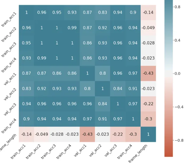
Table 2 show model accuracy after the introduced changes. We can see that the model indeed learns slower as was expected. We can also see small increase in validation accuracy, suggesting that the model indeed was overfitting the training data set and that the model changes had a positive impact on the learning process, even though the validation accuracy still remained very low. In Figure 8 we can see new correlations between individual data parameters. After training the model with new parameters, we can see that training and validation accuracy is more closely correlated than before while time frame length had a slightly smaller negative impact on the model accuracy.
In the next step, optimization algorithm was changed to observe the impact on learning rate and accuracy. The RMSProp algorithm, which was originally used as the network optimization algorithm was changed to Adaptive Moment Estimation (Adam), an improved version of the
RMSProp algorithm [22]. The accuracy achieved after changing the optimization algorithm can
be seen in Table 3 and the correlation matrix is shown in Figure 9. We can see that the effect on the accuracy and correlations is only marginal.
Training accuracy epoch 1 (%) Training accuracy epoch 2 (%) Training accuracy epoch 3 (%) Training accuracy epoch 4 (%) Validation accuracy epoch 1 (%) Validation accuracy epoch 2 (%) Validation accuracy epoch 3 (%) Validation accuracy epoch 4 (%) Time frame length (hours)
Failure type Train type
73.4 82.8 85.8 86.8 27.6 31.4 29.4 28.4 12 Compressor Electric 64.0 71.2 73.6 75.2 10.6 15.6 12.0 10.4 12 Pantograph Electric 72.6 82.6 85.2 86.8 29.4 29.0 30.2 29.6 4 Compressor Electric 63.8 70.4 72.8 74.6 23.4 16.8 18.0 19.6 4 Pantograph Electric 73.4 82.8 85.6 87.4 31.6 22.8 35.0 28.8 8 Compressor Electric 64.0 71.0 73.2 74.8 14.8 14.4 14.2 14.0 8 Pantograph Electric 64.0 70.2 72.0 73.4 12.4 11.0 12.8 10.8 12 Compressor Diesel 69.4 73.2 74.6 75.0 21.4 13.4 19.2 17.0 4 Compressor Diesel 64.6 70.0 72.2 73.4 14.2 11.8 14.4 12.2 8 Compressor Diesel
Table 2: Model accuracy after introducing dropout and changing activation function to sigmoid
Figure 8: Correlation matrix after introducing dropout and changing activation function to sigmoid
7.3.
Failure prediction
Results achieved for failure diagnosis were used to choose data parameters values and prediction model settings for failure prediction. Instead of training the model using all of the original input data parameters values, only the subset chosen in subsubsection 7.2..1 was used to reduce the computational power needed. The same model architecture as was used for further experimentation in subsubsection 7.2..1 was used for failure prediction. The architecture consisted of an LSTM and
Training accuracy epoch 1 (%) Training accuracy epoch 2 (%) Training accuracy epoch 3 (%) Training accuracy epoch 4 (%) Validation accuracy epoch 1 (%) Validation accuracy epoch 2 (%) Validation accuracy epoch 3 (%) Validation accuracy epoch 4 (%) Time frame length (hours)
Failure type Train type
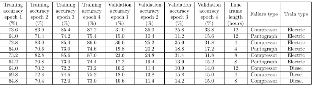
73.6 83.0 85.4 87.2 31.0 35.0 25.8 33.8 12 Compressor Electric 64.0 71.4 74.2 75.4 15.0 10.4 11.2 15.6 12 Pantograph Electric 72.8 83.0 85.4 86.6 30.6 25.2 35.0 31.8 4 Compressor Electric 64.0 70.6 73.0 74.6 19.8 20.2 18.8 17.2 4 Pantograph Electric 73.2 82.8 85.6 87.0 23.6 24.8 31.4 31.8 8 Compressor Electric 64.2 70.8 73.0 74.4 17.2 19.4 13.0 15.2 8 Pantograph Electric 64.0 70.2 72.2 73.2 10.2 11.4 10.0 14.0 12 Compressor Diesel 69.8 72.8 74.6 75.2 18.0 13.8 15.8 15.0 4 Compressor Diesel 64.8 70.4 72.0 73.0 10.6 11.4 14.2 15.0 8 Compressor Diesel
Table 3: Model accuracy after changing the optimization algorithm to Adam
a Dense layer, dropout was set to 0.5 and RMSProp was used as the optimization algorithm, since using Adam had very small impact on the learning rate.
The results for failure prediction can be seen in Table 4. The results are very similar to failure diagnosis, the model is able to learn how to predict failures using the training data set, but is unable to generalize and correctly classify new data. By looking at the correlation matrix in Figure 10, we can see that the correlation between individual parameters is also very similar to the initial results; decreasing the amount of information by increasing the time frame length has a negative impact on the model accuracy, while allowing a wider window for the failure position (marked as days preceding in the figure) has a small positive impact.
Training accuracy epoch 1 (%) Training accuracy epoch 1 (%) Training accuracy epoch 1 (%) Training accuracy epoch 1 (%) Validation accuracy epoch 1 (%) Validation accuracy epoch 1 (%) Validation accuracy epoch 1 (%) Validation accuracy epoch 1 (%) Validation accuracy epoch 1 (%)
Days preceding Failure type Train type
68.4 78.8 82.2 84.0 26.4 37.0 24.0 31.2 12 2 4 R 68.0 78.2 81.8 84.0 19.0 32.4 36.8 32.4 12 4 4 R 60.6 68.0 70.2 72.4 29.8 13.2 11.8 17.8 12 2 5 R 60.6 67.6 70.4 72.2 27.8 18.0 18.2 15.4 12 4 5 R 68.0 78.6 81.8 83.4 33.8 29.6 27.6 32.4 4 2 4 R 67.6 77.4 81.0 82.8 32.0 35.0 34.6 36.6 4 4 4 R 60.0 67.0 69.8 71.4 30.4 18.2 16.0 17.0 4 2 5 R 60.8 66.6 70.4 72.0 24.2 21.0 25.0 20.4 4 4 5 R 67.8 78.0 82.0 83.8 35.8 33.6 23.0 34.2 8 2 4 R 68.0 78.4 82.0 84.0 18.0 30.8 28.8 31.4 8 4 4 R 60.8 67.0 70.0 72.4 15.8 14.0 11.8 13.4 8 2 5 R 61.0 67.4 70.6 71.6 21.0 25.0 23.4 15.8 8 4 5 R 61.2 66.2 68.4 70.6 11.6 8.4 12.0 10.0 12 2 4 T 62.6 67.8 69.2 70.8 15.6 12.0 16.0 12.2 12 4 4 T 66.8 70.6 72.2 72.6 31.4 17.0 13.6 14.2 4 2 4 T 98.6 100.0 100.0 100.0 49.0 49.0 49.0 49.0 4 4 4 T 61.8 67.2 69.2 70.6 13.4 13.6 10.8 10.6 8 2 4 T 66.8 70.6 71.8 72.6 26.8 23.4 14.6 14.2 8 4 4 T
8.
Discussion
8.1.
Answers to research questions
1. What are the most important factors in the data that are currently being collected with respect to predictive data analysis?
The most important factor is the quality of the data. In order to create and train a reliable failure prediction model, the data must be as accurate as possible and there must be enough data to enable the model to learn general patterns. In this thesis, the data was not completely accurate and classes in the data set were out of balance and the combination of those two issues might have led to the failure to properly train the prediction model.
The next factor to consider is the choice of machine learning algorithm. RNNs were used in this thesis, as they have been successfully used in the past for similar problems, but convolutional NNs also seem to be a good candidate.
2. How do the data need to be processed in order to be used for machine learning algorithms? This thesis transformed the events data into temporal sequences, in which each value repre-sented amount of occurrences of a specific event during a time frame. This way, the problem can be turned into a sequence classification task.
3. Why are the currently collected data unsuitable for predictive analysis and what would need to change in terms of data collection in order to allow predictive analysis in the future? As mentioned in subsection 8.2., the failures data collected suffered from several issues. Failures need to be categorized as soon as they are recorded, currently the failure reports contain only short hand written description which has to be categorized retrospectively and this introduces a lot of room for error, as for each report it has to be determined whether it was a failure or not and whether it falls into a certain category or not.
Using sensor data should also be considered, as that is the usual way of predicting hardware related failures (examples of research papers dealing with this problem are presented in section 3.). The data however needs to be recorded either continuously or at least on a regular basis with sufficient frequency to ensure that essential information is captured. Neither of those is available at the moment, which is one of the reasons that the sensor data was not analyzed at all in this study.
4. What is the most suitable machine learning algorithm for failure prediction based on events data?
In this study LSTM NN, an implementation of a RNN was used. This algorithm was able to learn how to classify the training data set, however it was not able to generalize the patterns and apply them on a new data set. Nevertheless, it cannot be easily determined whether this was due to a wrong choice of the prediction model architecture or due to the data set used to train the model, therefore all that can be said is that recurrent NNs and LSTM networks in specific are a good candidate, but further research needs to be done to determine how suitable this algorithm actually is for this task.
8.2.
Threats to validity
The result of this study could be strongly influenced by the quality of the data set, which suffers from two significant deficiencies. First, the amount of failures collected over the two year period was very low; in the best case the number of failures was only 138 (in the case of pantograph failures), which is a very low number to train any machine learning algorithm. To increase the number of inputs representing a failure, a variation of the SMOTE approach was conducted, however this approach did not create new unique inputs, it only produced slightly different copies of the original values, which brought little value except balancing the data set classes at the cost of increasing the risk of overfitting.
The other deficiency of the data set is the failure collection and categorization process. The failures were collected in the form of a hand written report, meaning that the detail and accuracy
of the information contained in the report was strongly influenced by the individual personnel responsible for writing the reports, making the categorization task more difficult and introducing the risk of either missing out on some failure reports or wrongly classifying others. The reports also did not contain the exact time of the failure occurrence, they only contained the time when the failure report was created. Even though the failures usually happen no longer than 24 hours and almost never more than 48 hours before the report is written, this variation still introduces uncertainty about how long before the report did the failure actually happen and consequently how should be the data labeled.
8.3.
Future work
In this study, only information about how many times a certain event occurred during a time frame of specified length was considered. However, some events also have duration, which could provide the additional information needed to be able to accurately diagnose or predict failures. Sensor data could be also considered, either separately or in addition to events data. The train system, on which data were collected for this study, records sensor data only shortly (usually a few seconds or at most several minutes) after an event occurs. This again introduces the problem of discontinuous stream of information, however the information provided directly measures a hardware condition, which could be more important than the event itself, even though sometimes the event can be a consequence of changes in the hardware conditions. Another drawback of this approach is that the amount of data generated by sensors is much larger that the amount generated just by events, therefore more computational resources would be needed to analyze the data and even then, it would probably be necessary to reduce the amount of data by extracting only some features of the signal.
The approach introduced in this study did not take into consideration whether a specific event contains any information that could be used for diagnosis or not, data about all events were used. The main reason for this was the lack of information about individual events, as it was not known which events signal an unusual activity which could lead to a failure, it was only known that some events certainly do not carry any useful information (such as fuel measuring), as they happen on a regular basis regardless of outer influences. Taking into account all events unnecessarily increases the amount of data that needs to be preprocessed and later used for training, which not only increases the computational resources, but also potentially introduces information which makes it more difficult for the prediction model to learn. In future, additional information about individual events could be collected, so that events which are known not to contain any useful information are not used at all.
The prediction model used in this thesis consisted of only one recurrent LSTM layer and one
dense layer, several research papers [23, 24] have however combined recurrent and convolutional
NNs for sequence classification. Similar approach could be tried on the data set used in this thesis to further examine whether the low validation accuracy achieved was the result of wrong a model architecture or an unsuitable data set.
9.
Conclusions
This thesis introduced an approach to process train events data and use them for machine learning algorithms in order to diagnose and predict failures. Event occurrences were counted for individual time frames in the two year period, for which data were available, and the time frames were grouped into periods of several weeks to create individual inputs for the machine learning algorithm. This way, the problem can be turned into a sequence classification task. Recurrent neural networks were chosen as the most appropriate machine learning algorithm, as they are capable of capturing temporal behaviour in the data and, in specific, an LSTM layer was used in the prediction model, as it is better at handling long sequences of data. The model was able to achieve high training accuracy for both failure diagnosis and prediction, however it was unable to generalize the patterns, which resulted in a very low validation accuracy. The most likely reason for this was overfitting caused by the small amount of data regarding failures. Other aspects which need to be considered are missing information in the data, which would mean that failure diagnosis and prediction is impossible using the currently available events data, which suffers from several deficiencies (see subsection 8.2.). Last, the proposed prediction model architecture might be inappropriate for this task, meaning that it either has to be improved or completely changed. To prove or disprove any of these hypotheses, further research needs to be done.
References
[1] C. Turner, C. Emmanouilidis, T. Tomiyama, A. Tiwari, and R. Roy, “Intelligent decision support for maintenance: an overview and future trends,” International Journal of Computer Integrated Manufacturing, vol. 32, 10 2019.
[2] “ADDIVA-EEPAB Gruppen.”https://www.addiva.se/. Accessed on January 5, 2020.
[3] N. Sakib and T. Wuest, “Challenges and opportunities of condition-based predictive mainte-nance: A review,” vol. 78, pp. 267–272, 2018.
[4] E. Veronese, U. Castellani, D. Peruzzo, M. Bellani, and P. Brambilla, “Machine learning approaches: From theory to application in schizophrenia,” Computational and Mathematical Methods in Medicine, vol. 2013, 2013.
[5] G. J. Myatt, Making Sense of Data: A Practical Guide to Exploratory Data Analysis and Data Mining. USA: Wiley-Interscience, 1st ed., 2006.
[6] S. Hochreiter and J. Schmidhuber, “Long short-term memory,” Neural Computation, vol. 9, no. 8, pp. 1735–1780, 1997.
[7] C. Olah, “Understanding LSTM Networks.” http://colah.github.io/posts/
2015-08-Understanding-LSTMs/, Aug. 2015. Accessed on June 6, 2020.
[8] “Scopus.”https://www.scopus.com/. Accessed on January 25, 2020.
[9] R. Jegadeeshwaran and V. Sugumaran, “Brake fault diagnosis using clonal selection classifica-tion algorithm (csca) – a statistical learning approach,” Engineering Science and Technology, an International Journal, vol. 18, no. 1, pp. 14–23, 2015.
[10] V. Indira, R. Vasanthakumari, R. Jegadeeshwaran, and V. Sugumaran, “Determination of minimum sample size for fault diagnosis of automobile hydraulic brake system using power analysis,” Engineering Science and Technology, an International Journal, vol. 18, no. 1, pp. 59–69, 2015.
[11] U. Shafi, A. Safi, A. Shahid, S. Ziauddin, and M. Saleem, “Vehicle remote health monitoring and prognostic maintenance system,” Journal of Advanced Transportation, vol. 2018, 2018. [12] F. P. G. Marquez, P. Weston, and C. Roberts, “Failure analysis and diagnostics for railway
trackside equipment,” Engineering Failure Analysis, vol. 14, no. 8, pp. 1411 – 1426, 2007. [13] H. Yilboga, O. Eker, A. G¨u¸cl¨u, and F. Camci, “Failure prediction on railway turnouts using
time delay neural networks,” pp. 134–137, 2010.
[14] O. Fink, E. Zio, and U. Weidmann, “Predicting time series of railway speed restrictions with time-dependent machine learning techniques,” Expert Systems with Applications, vol. 40, no. 15, pp. 6033–6040, 2013.
[15] O. Fink, U. Weidmann, and E. Zio, “Extreme learning machines for predicting operation disruption events in railway systems,” pp. 1781–1787, 2014.
[16] N. Chawla, K. Bowyer, L. Hall, and W. Kegelmeyer, “Smote: Synthetic minority over-sampling technique,” Journal of Artificial Intelligence Research, vol. 16, pp. 321–357, 2002. [17] M. Soni, I. Sheikh, and S. Kopparapu, “Label-driven time-frequency masking for robust speech
command recognition,” Lecture Notes in Computer Science (including subseries Lecture Notes in Artificial Intelligence and Lecture Notes in Bioinformatics), vol. 11697 LNAI, pp. 341–351, 2019.
[18] G. Klarenbeek, R. Harmanny, and L. Cifola, “Multi-target human gait classification using lstm recurrent neural networks applied to micro-doppler,” vol. 2018-January, pp. 167–170, 2017.
[19] Y.-F. Hsu, M. Ito, T. Maruyama, M. Matsuoka, N. Jung, Y. Matsumoto, D. Motooka, and S. Nakamura, “Deep learning approach for pathogen detection through shotgun metagenomics sequence classification,” Lecture Notes in Computer Science (including subseries Lecture Notes in Artificial Intelligence and Lecture Notes in Bioinformatics), vol. 11526 LNAI, pp. 24–30, 2019.
[20] “Pythong programming language - official website.”https://www.python.org/. Accessed on
February 2, 2020.
[21] “Keras: The Python Deep Learning library.” https://keras.io/. Accessed on April 28,
2020.
[22] M. Stewart, “Neural Network Optimization.” https://towardsdatascience.com/
neural-network-optimization-7ca72d4db3e0, June 2019. Accessed on May 9, 2020. [23] J. Wang, W. Wang, S. Wei, Y. Zeng, and F. Luo, “Time series sequences classification with
inception and lstm module,” pp. 51–55, 2019.
[24] P. Chong, Y. Elovici, and A. Binder, “User authentication based on mouse dynamics using deep neural networks: A comprehensive study,” IEEE Transactions on Information Forensics and Security, vol. 15, pp. 1086–1101, 2020.
A
Python code for the prediction model
i m p o r t k e r a s
i m p o r t numpy
# l o a d y o u r d a t a s e t h e r e , n o t e t h a t i t must be a numpy a r r a y , # i f i t i s a r e g u l a r python c o l l e c t i o n , you can j u s t c a l l # y o u r d a t a = numpy . a r r a y ( y o u r d a t a ) # t o c o n v e r t i t t o a numpy a r r a y # i n i t i a l i z e t h e model model = k e r a s . S e q u e n t i a l ( ) # add an LSTM l a y e r t o c a p t u r e t e m p o r a l b e h a v i o u r f o r e a c h e v e n t model . add ( k e r a s . l a y e r s .LSTM( # d i m e n s i o n a l i t y o f t h e o u t p u t s p a c e , i n o u t c a s e one f o r e a c h e v e n t n u m b e r o f e v e n t s , # s h a p e o f t h e i n p u t d a t a
# we have one row f o r e a c h t i m e f r a m e and one column f o r e a c h e v e n t
i n p u t s h a p e =( f r a m e s p e r p e r i o d , n u m b e r o f e v e n t s ) , # a c t i v a t i o n f u n c t i o n s a c t i v a t i o n= ’ s i g m o i d ’ , r e c u r r e n t a c t i v a t i o n= ’ s i g m o i d ’ , # d r o p o u t s d r o p o u t = 0 . 5 , r e c u r r e n t d r o p o u t = 0 . 5 , # p e r f o r m a n c e o p t i m i z a t i o n c h o i c e , d e p e n d s on hardware i m p l e m e n t a t i o n=1 ) ) # add a d e n s e l a y e r on t o p o f t h e l s t m l a y e r
model . add ( k e r a s . l a y e r s . Dense (
# o u t d i m e n s i o n a l i t y , i n o u r c a s e v a l u e between 0 and 1 1 , # a c t i v a t i o n f u n c t i o n a c t i v a t i o n= ’ s i g m o i d ’ ) ) # s e t o p t i m i z e r , l o s s f u n c t i o n and a c c u r a c y m e a s u r e s f o r t h e model model .c o m p i l e( o p t i m i z e r= ’ rmsprop ’ , l o s s=t f . k e r a s . l o s s e s . B i n a r y C r o s s e n t r o p y ( ) , m e t r i c s =[ t f . k e r a s . m e t r i c s . B i n a r y A c c u r a c y ( ) , t f . k e r a s . m e t r i c s . F a l s e P o s i t i v e s ( ) , t f . k e r a s . m e t r i c s . F a l s e N e g a t i v e s ( ) , t f . k e r a s . m e t r i c s . T r u e P o s i t i v e s ( ) , t f . k e r a s . m e t r i c s . T r u e N e g a t i v e s ( ) , ] ) n e p o c h s = 4
# t r a i n t h e model u s i n g t h e i n p u t data , i n p u t s and l a b e l s must be s e p a r a t e
# t h e h i s t o r y c o n t a i n s i n f o r m a t i o n ab ou t model a c c u r a c y a f t e r e a c h ep oc h d u r i n g t r a i n i n g h i s t o r y = model . f i t ( # i n p u t d a t a x=t r a i n i n p u t s , # l a b e l s f o r t h e i n p u t d a t a y=t r a i n l a b e l s , # number o f e p o c h s e p o c h s=n e p o c h s , # l o g g i n g c o n f i g u r a t i o n , h a s no e f f e c t on t r a i n i n g v e r b o s e =1 , # s h u f f l e t h e i n p u t d a t a s h u f f l e=True , # v a l i d a t i o n d a t a s e t v a l i d a t i o n d a t a =( t e s t i n p u t s , t e s t l a b e l s ) , # t r a i n i n g i n b a t c h e s i m p r o v e s p e r f o r m a n c e b a t c h s i z e =64
)