http://www.diva-portal.org
Postprint
This is the accepted version of a paper presented at TAP - Transportation and Air Pollution.
Citation for the original published paper:
Lundberg, J., Blomqvist, G., Gustafsson, M., Janhäll, S. (2017)
Texture influence on road dust load
In: Proceedings of the 22nd International Transportation and Air Pollution Conferens
(pp. 14-).
N.B. When citing this work, cite the original published paper.
Permanent link to this version:
Conference Proceedings
Contents:
(click titles to navigate)
Vehicle Emissions
1. Update of Emission Factors for EURO 6 Diesel Passenger Cars for the HBEFA 2. Variations of Real-world NOx Emissions of Diesel Light Commercial Vehicles
3. Comparison of regulated emission factors of Euro 6-LDV in Nordic temperatures and cold start conditions: Diesel-DI and Gasoline-DI
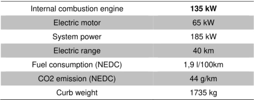
4. Measurement and simulation of hybrid and plug in hybrid vehicles for the handbook of emis-sion factors
5. A novel approach for NOx emission factors of diesel cars in HBEFA
6. Assessment of risks for elevated NOx emissions of diesel vehicles outside the boundaries of RDE
7. Plume Chasing NOx RDE Measurements to Identify Manipulated SCR Emission Systems of Trucks
8. Analysis of tail-pipe emissions of a plug-in hybrid vehicle and its average emissions for differ-ent test cycles
9. Particle Number Emissions of Euro 6 Light Duty Vehicles
10. Dilution effects on ultrafine particle emissions from Euro 5 and Euro 6 diesel and gasoline ve-hicles
Road Side Particles
1. On-road measurements of particles from tire-road contact 2. Texture influence on road dust load
3. Wear particle emissions from cement concrete pavement
4. Non-exhaust PM10 traffic emissions, road dust loading and the impact of dust binding – appli-cation of the NORTRIP emission model
Non Road Emissions
1. PACLA (PArticle CLAssifier): A Novel Approach for Quantification and Differentiation of Prima-ry Particulate Matter (PM) Emitted by Road and Railway Transport
2. Particle and gaseous emissions from a dual-fuel marine engine
3. Maritime Emissions for Different Emission Reduction Scenarios in the Arctic
CO2 Emissions of Road Traffic
1. CO2 emissions of the European Heavy Duty Truck Fleet, a Preliminary Analysis of the Ex-pected Performance Using VECTO Simulator and Global Sensitivity Analysis Techniques 2. On-road determination of a reference CO2 emission for passenger cars
3. Estimating the European Passenger Car Fleet Composition and CO2 Emissions for 2030
Remote Sensing
1. Quantification of vehicle cold start effects on NOx and NO2 emissions using remote sensing 2. Thousands of snapshots vs. trips with thousands of seconds – how remote sensing
comple-ments PEMS/chassis emission measurecomple-ments
3. Pan-European study on real-driving NOX emissions from late model diesel cars as measured by remote sensing
Non-European Studies
2. Emissions of regulated and unregulated pollutants from light-duty gasoline vehicles using dif-ferent ethanol blended fuels
3. Air Quality and Health Benefits from Fleet Electrification in China: Future Perspectives through 2030
Air Quality and Health Impact
1. An Efficient Scheme for Urban Air Quality Estimates and Projections 2. Effects of traffic related abatement policies on Swiss air quality trends 3. Comprehensive analysis of European vehicular primary NO2 trends
4. Health impact of PM10, PM2.5 and BC exposure due to different source sectors in Stockholm, Gothenburg and Umea, Sweden
5. Impact of excess NOx emissions from diesel cars on air quality, public health and eutrophica-tion in Europe
6. Impacts and mitigation of excess diesel-related NOx emissions in 11 major vehicle markets
Air Traffic Particles
1. Assessment of particle emissions from aircraft turbine engines: ground, cruise, and overall flight emissions
2. Impact of alternative fuels on the non-volatile particulate matter mass and number emissions of an aero gas turbine
3. Chemical composition and toxicological properties of ambient particles (PM0.25) from near-airport and urban road traffic sites
Large Scale Emission Data
1. Emission estimation based on cross-sectional traffic data
Update of Emission Factors for EURO 6 Diesel Passenger Cars for the
HBEFA
C. Matzer1, S. Hausberger1, M. Rexeis1, M. Opetnik1, M. Ramsauer1, O. Mogg1 and F. Weger1
1 Institute for Internal Combustion Engines and Thermodynamics, Graz University of Technology, A-8010 Graz, Austria, matzer@ivt.tugraz.at
Abstract
The HBEFA (The Handbook Emission Factors for Road Transport) provides emission factors for road vehicles on several traffic situations for different countries in Europe. The emission factors are based on simulation data for various HBEFA cycles. The simulation is done by the software PHEM (Passenger car and Heavy duty Emission Model) using emission maps created from measurement data.
The last HBEFA update 3.2 was published in July 2014 including already EURO 6 emission classes for diesel and petrol cars based on a limited amount of measured passenger cars, which were available at that time. It was noted, that especially NOx emissions from the small measured sample may not be representative for the EURO 6 diesel car fleet. Therefore, the HBEFA version 3.3 has been produced and was released in April 2017.
For the HBEFA 3.3 in PHEM a new method to produce engine emission maps from test data (“CO2 interpolation method”) was used. With this method, it is possible to consider also measurement data where the engine load signal is not available or too inaccurate for engine map creation. This is especially useful for RDE (Real Driving Emissions) measurements, where the engine power signal in most of the cases is not available. Using RDE measurements beside chassis dynamometer test data increase the sample size of tested vehicles and improve in general the representativeness of the engine emission maps.
With the extended pool on measurement data due to additional RDE trips, also investigations like ambient temperature influence on NOx emissions were realised. For that purpose, the measurement data of several conventional diesel EURO 6 cars at different ambient temperatures on road and on chassis dynamometer were used.
To analyse the ambient temperature effect on NOx isolated from influences of routes and driver behaviour, separate engine emission maps with RDE data measured at different ambient temperatures were created by PHEM with the CO2 interpolation method. With these maps the CADC (Common Artemis Driving Cycle) was simulated for each vehicle. The different results for the CADC using the maps from different ambient temperatures provide a common basis for the analysis of temperature influences on emissions. Since the CADC is representative for real world driving, the result for the temperature effects shall also be valid for real emission behaviour. The analysis showed a high sensitivity of NOx emissions against ambient temperature, e.g. from 20 °C to 10 °C the NOx emissions increase approximately 40 % to 50 %. This high sensitivity was the reason for further investigations based on remote sensing and finally for the implementation in HBEFA 3.3.
For HBEFA 4.1 – which is planned to be elaborated until 2019 – additional investigations regarding ambient temperatures are taken into account. Also investigations with a detailed EAS (Exhaust After-treatment System) model in the PHEM simulation are performed. The EAS simulation may improve the accuracy especially in low load cycles and cold environment since all HBEFA simulations for cars are based on EoT (End-of-Tailpipe) data so far. Special traffic situations, e.g. stop&go traffic or coasting followed by high load phases can result in relative high NOx levels due to low conversion efficiency resulting from cool down phases of the EAS if the engine has no special heating strategies. To parametrise the SCR (Selective Catalytic Reduction) model in PHEM for such effects measurements in stop&go cycles were performed at TUG (Graz University of Technology).
Introduction
The last HBEFA (Handbook Emission Factors for Road Transport) update was published in July 2014. In the update already the EURO 6 emission classes for diesel and petrol cars based on available measurements of a few passenger cars were included, but it was noted, that especially NOx emissions from the small measured sample may not be representative for the future EURO 6 fleet. In the meantime, several unexpected software features in diesel emission control systems were detected on one hand and the RDE legislation came in place on the other hand, which shall better control real world emission behaviour of cars.
To check and to update the EURO 6 emission factors with all vehicle emission tests at diesel EURO 6 cars collected around Europe since HBEFA 3.2, the HBEFA 3.3 has been produced. In the course of the work a first assessment of ambient temperature dependency of the NOx emission factors was made. HBEFA 3.3 is a so-called “quick update”, because only the NOx emission factors for conventional diesel passenger cars have been revised. An update for all exhaust gas components is planned for HBEFA 4.1. Following adaptations from HBEFA 3.2 to 3.3 have been performed:
New emission factors of EURO 6, EURO 6d-Temp and EURO 6d diesel passenger cars replace the previous emission factors of EURO 6 and EURO 6c from HBEFA 3.2. New NOx emissions factors of EURO 4 diesel cars replace the old ones from HBEFA 3.2.
Due to the low effect on the NOx emission behaviour these results are not be presented in this paper, details are described in the HBEFA report (Hausberger S., Matzer C. 2017), (Keller M., et. al. 2017).
A correction function for the influence of ambient temperature on NOx emissions for EURO 4, EURO 5 and EURO 6 diesel cars was introduced.
The update is based on RDE (Real Driving Emissions) and chassis dynamometer measurements. For the effect of ambient temperature on NOx emissions, also remote sensing data were used. For HBEFA 4.1 following investigations are ongoing for further improvement of the robustness and accuracy of the emission model PHEM:
Additional investigations regarding ambient temperature effect on NOx emission behaviour.
Generic CO2 engine map calibration for the CO2 interpolation method.
Detailed EAS (Exhaust After-treatment System) simulation to reflect effects of low load driving conditions.
Used simulation tool and method for update of HBEFA emission factors
The emission factors are based on the simulation of a huge number of driving situations and vehicle categories with the simulation tool PHEM (Passenger car and Heavy duty vehicle Emission Model). PHEM is an engine emission map based instantaneous emission model, which has been developed by TUG (Graz University of Technology) since the late 1990's. It calculates fuel consumption and emissions of road vehicles in 1 Hz time resolution for a given driving cycle. The model has already been presented in several publications, e.g. (Hausberger S. et. al. 2009), (Zallinger M. 2010), (Rexeis M. et. al. 2009), (Luz R., Hausberger S. 2009). PHEM simulates the engine power necessary to overcome the driving resistances based on the vehicle longitudinal dynamics, losses in the drive train and power demand to run basic auxiliaries in 1 Hz over any driving cycle. The engine speed is simulated by the transmission ratios and a driver gear shift model. Then basic emission values are interpolated from the engine emission maps. Depending on the vehicle technology, the status of the EAS and dynamic effects on the emission level are considered to increase the model accuracy. With this approach, realistic and consistent emission factors can be simulated for any driving condition since the main physical relations are taken into consideration. E.g. variations in road gradients and in vehicle loading influence the engine power demand and the gear shift behaviour and thus lead to different engine loads over the cycle.
To simulate representative fleet average emissions per vehicle class, representative engine maps are necessary. PHEM produces emission maps by sorting the instantaneously measured emissions into standardised maps according to the actual engine speed and power. To produce representative engine maps from vehicle tests, many vehicles should be included and realistic driving situations should be considered. Consequently, the inclusion of PEMS (Portable Emission Measurement System) data by a newly developed methodology in addition to the chassis dynamometer data is very beneficial for a broader vehicle sample for the PHEM simulation. The new method resolves the typical issue from PEMS tests, where most often no reliable engine torque signal is available. PHEM offers the option to calculate the engine power from the measured CO2 mass flow and engine speed based on generic engine CO2 emission maps (Figure 1). These generic maps for different emission concepts have been acquired in a project together with Ricardo-AEA for the European Commission (Hill N., et. al. 2015). These maps contain engine speed, CO2 flow and engine power relations for different engine technologies. Thus, only the measured engine speed and emissions are necessary to compile engine emission maps. This method, also called “CO2 interpolation method”, was already presented at the International Transport und Air Pollution Conference in Lyon 2016 (Matzer C. et. al. 2016).
Figure 1: Example for interpolation of engine power from a generic CO2 map.
The accuracy of the CO2 interpolation method can be tested by comparing measurement results for cycles driven on the chassis dynamometer with simulation results based on the generic CO2 maps for these cycles. When the test mass and road load values from the chassis dynamometer setting are used as input for the PHEM simulation, the difference to the measured CO2 results from:
Deviations of the vehicle specific map to the generic map.
Differences in the generic model for losses in the gear box and the axle.
Differences in the real auxiliary power demand to the generic data used in PHEM. For the HBEFA 3.3 update only a few results from chassis dynamometer tests were analysed. These showed a CO2 uncertainty of the generic diesel EURO 6 map up to 20 % using default values for auxiliary power demand and losses in the gear box and the axle. For the quick update no calibration of the generic fuel maps was applied. Deviations in the generic maps lead to inaccurate allocation of the instantaneous emissions to the instantaneous engine power and thus give less reliable emission maps. Therefor for HBEFA 4.1 a calibration of the generic maps in PHEM was developed. By calibrating the PHEM model data to meet the measured CO2 values, a more representative generic data set can be established. The calibration of the generic or base CO2 maps is provided for each vehicle used in HBEFA 4.1 where the required data for calibration are available from chassis dynamometer tests. The method for the map calibration is described in the following. Real world cycles including high load operating points like CADC (Common Artemis Driving Cycle), RWC (Real World Cycle) or an ERMES (European Research group on Mobile Emission Sources) cycle can be used for generic map calibration. Using the mass and road load settings from the chassis dynamometer tests PHEM recalculates the tests with the generic CO2 map. For calibration of the generic map, the simulated CO2 flow is compared with the measured one. To calibrate the “hot” generic maps only measurement data should be used where the engine is at operating temperature. Figure 2 shows the measured (grey points) and simulated normalized CO2 values (black points) over normalized engine power for a single diesel passenger car in the CADC. Normalized means, that CO2 and engine power are divided by rated
power. Since this CADC was cold started, the urban phase was not considered for map calibration. Each dot represents the CO2 and engine power average over 20 s to avoid uncertainties regarding time alignment due to different gas delay times from engine out to the analysers in full load and idling operating points. The trend lines are described very well by linear equations. These linear equations are called “Veline” (Vehicle efficiency line) and were used already in the past at TUG, e.g. for WLTP corrections (Hausberger S., et. al. 2015) and for corrections in a HVAC (Heating, Ventilation and Air Conditioning) test procedure (Hausberger S., et. al. 2013). The Velines are similar to the well-known Willans-lines but are not restricted to a constant engine speed but to the engine speed range defined by the gear shift logics driven in the cycle. Based on the difference in the Velines functions from measured and simulated data, the calibration function can be determined.
Figure 2: 20 s average of measured and simulated CO2 and engine power on CADC using the base CO2 map.
Figure 3: 20 s average of measured and simulated CO2 and engine power on CADC using calibrated CO2 map.
To calibrate the generic or base CO2 map the correction could be done by adding or multiplying a correction function. Investigations showed less uncertainties if the correction function is added. For the data shown in Figure 2 the correction function reads as follows:
CO2_meas(Pnorm) = 688.1744 * Pnorm + 13.9196 …vehicle specific function Formula 1 CO2_sim(Pnorm) = 613.1472 * Pnorm + 13.5741 …vehicle specific function Formula 2 ∆CO2_corr(Pnorm) = CO2_meas(Pnorm) – CO2_sim(Pnorm) Formula 3 CO2_corr(Pnorm) = CO2_base(Pnorm) + ∆CO2_corr(Pnorm) …valid for Pnorm >0 Formula 4 The correction will be done only for normalized engine power >0 to have no influence on the engine drag curve where the CO2 is zero due to trailing throttle fuel cut-off. Figure 3 shows the simulation result after map calibration. The measured data are similar to the data shown in Figure 2. After the calibration, the trend lines of the measured and simulated data are nearly congruent. Also the CO2 dependency on engine speed was examined, but this results in less than 1 % improvement of simulated CO2 for the investigated vehicles. Therefore, no additional calibrations over engine speed are performed. The method of CO2 map calibration was applied to 3 diesel EURO 6 vehicles so far to test the uncertainties resulting from the generic CO2 map method. Since for vehicles measured with PEMS only, no calibration of the map is possible, the remaining uncertainty could lead to a less reliable emission map. Table 1 shows the cycles used for map calibration as well as cycles, which were used for validation. As mentioned, the calibration and validation is performed only with cycle data where the engine worked under warm conditions. The ambient temperature was 23 °C for all cycles listed in Table 1.
Table 1: Diesel EURO 6 vehicles used for the calibration of the generic diesel CO2 map. ID Segment Odometer [km] Rated engine power [kW] Used cycle for calibr. Simulated cycles
Veh_a C-Segment 34000 81 CADC 1x WLTC, 1x CADC Veh_b C-Segment 1300 96 RWC 2x WLTC, 1x RWC
Veh_c N1-III 6000 132 Ermes 2x WLTC, 1x ERMES, 2x RWC The results for CO2 and NOx are shown in Figure 4 and Figure 5 for the mentioned cycles.
For all 3 vehicles the base CO2 map underestimates the measured CO2. As expected, the CO2 deviations between measurement and simulation is decreasing after calibration, independent which cycle for calibration is used. The CO2 map calibration influences also the NOx map creation using the CO2 interpolation method. For these vehicles the NOx simulation with the calibrated maps result consequently in higher NOx. This is referable to the “poorer” CO2 maps used for the CO2 interpolation method assuming that the measured NOx increase with increasing engine power.
Figure 4: Comparison of simulated and measured CO2 for 3 different diesel EURO 6 vehicles.
Figure 5: Comparison of simulated and measured NOx for 3 different diesel EURO 6 vehicles.
In Figure 6 and Figure 7 the average CO2 and NOx deviations between simulation and measurement for the listed cycles in Table 1 are presented for each vehicle. For the simulation the generic CO2 map (= base map, which is the same for all 3 vehicles) as well as the vehicle specific calibrated maps were used. Negative deviation means, that the simulation underestimates the measured values. Also an average deviation of all vehicles is shown, referred to as “Veh_a+b+c”. After map calibration the CO2 deviations are less than 5 %. The NOx deviations are between -20 % to 20 % using EoT (End-of-Tailpipe) maps without any NOx calibration. It has to be noted, that the map calibration described allocates also uncertainties in the power demand from auxiliaries to the calibration. Especially in low engine loads the auxiliaries can have a high share in the fuel consumption (correlates with CO2 emissions), but also vary broadly over time (e.g. smart alternator control) and between vehicle models. The differences in the engine maps of the vehicles are assumed to be less pronounced than the deviations between calibrated and not calibrated data shown in Figure 4.
Figure 6: Average CO2 deviations between simulation and measurement of all cycles per investigated vehicle.
Figure 7: Average NOx deviations between simulation and measurement of all cycles per investigated vehicle.
As mentioned above, the calibration method was not applied in the model PHEM for the quick update of passenger car NOx emissions in HBEFA 3.3. As long as the generic CO2 map used to produce the emission maps meets on average the CO2 map of the measured vehicles, the error
for the average engine emission map is small since errors from single vehicles are levelled out in the average map. For the 3 vehicles investigated here the effect of the calibration of the generic engine map is an increase in simulated NOx emissions by approximately 15 % (Figure 7). For HBEFA 4.1 it is planned to use calibrated CO2 maps where possible.
NO
xemission factors update for HBEFA 3.3
Table 2 gives an overview on the main specifications of the vehicles available for HBEFA 3.3 and the sources of the measured data. The registration numbers refer to the number of new registrations of the particular vehicle from 2013 to 2015 according to the EU-28 CO2 monitoring database. This is the timeframe where the EURO 6 cars have been introduced. Registration data for 2016 was not available during the work on the update of the PHEM model. The sample of measured vehicle models covers 18 % of the passenger car diesel models registered 2013 to 2015. The registration number is the basis for the weighting of the engine maps for the average engine emission map for PHEM. The registrations consider the number of new vehicles for the mentioned model as well as of variants of this model, e.g. Audi A4 Saloon or Audi A4 Avant. The assumption is that each vehicle in Table 2 represents the NOx emission behaviour for all model variants of this vehicle.
Table 2: Diesel EURO 6 vehicle measurements used in PHEM for HBEFA 3.3 update. Lab Make Model Rated engine power [kW] Rated engine speed [rpm] registrations [#] New
TUG BMW X5 180 4000 79756
TUG BMW 530d 180 4000 11851
TUG Audi A4 Allroad 180 4000 306698
TUG Mazda CX-5 110 4500 49514
TUG BMW 320d 120 4000 103691
TUG Kia Carens 104 4000 40461
TUG Audi Q7 160 4000 37221
TUG VW Sharan 110 3500 88353
TUG Peugeot 508 SW 88 3500 122878
EMPA VW Golf VII 81 3200 855277
EMPA Mazda CX-5 110 4500 49514
EMPA BMW 530d 190 4000 11851
EMPA Mercedes-Benz GLK 220 125 3200 48060
EMPA VW Passat 103 4200 459372
EMPA Renault Scenic 96 4000 278320
EMPA Mini Cooper 85 4000 18994
EMPA Mercedes-Benz A220 125 3400 17357
EMPA BMW X3 140 4000 95544
EMPA Mercedes-Benz ML 350 190 3600 34730
EMPA Porsche Macan 190 4000 25615
EMPA Peugeot 208 SW 110 3750 340831
ADAC BMW 118d 110 4000 103691
ADAC BMW 320d 140 4000 103691
TNO Ford Focus 70 3600 326974
To produce engine emissions maps following steps were executed. The steps should give a rough overview about the update, details are described in the HBEFA 3.3 report (Hausberger S., Matzer C. 2017), (Keller M., et. al. 2017).
1. Preparation of the available modal measurement data of CADC, ERMES, WLTC (Worldwide harmonized Light vehicles Test Cycle) and RWC. Additional to the chassis dynamometer measurements also data of RDE trips have been used. The preparation includes the work for correction of time shift between emissions and load signal, removal of cold start phases and selection of measured data where the average ambient temperature was between 15 °C and 30 °C. Test data at lower temperatures were used to analyse the influences of ambient temperature on NOx emissions as described later. 2. Engine map creation with the measurement data of each vehicle using the mentioned
CO2 interpolation method. To get one average diesel EURO 6 engine emission map, the single engine emission maps were weighted with the registration numbers listed in Table 2.
3. Calibration of the average EURO 6 engine emission map. The calibration has the target to calibrate the PHEM model, which is based on a limited sample of modal measurement data of vehicle tests to the broader sample of bag results stored in ERMES DB (database). Since the HBEFA 3.3 is a quick update for the NOx emission behaviour, the calibration was only done for NOx.
4. Simulation of HBEFA cycles with the average diesel EURO 6 car, which has a total vehicle mass of 1651 kg and an engine power of 99 kW.
5. Assessment of the EURO 6d-Temp and EURO 6d NOx emission behaviour considering the conformity factors for NOx on RDE tests.
With the PHEM parameterisation for emission behaviour of EURO 6, EURO 6d-Temp and EURO 6d diesel vehicles, emission factors for the full set of HBEFA driving cycles in combination with all road gradients have been calculated. Figure 8 shows the new NOx emissions results as function of the average vehicle velocity for the mentioned EURO classes for 0 % road gradient. The NOx emission results of EURO 6 from HBEFA 3.2 are plotted for comparison. The former EURO 6 emission factors of HBEFA 3.2 are between the actual EURO 6 and EURO 6d-Temp levels. When the emission factors for HBEFA 3.2 were produced, details of the RDE legislation were not defined. The update of emission factors thus improves the representativeness for EURO 6 due to the much larger sample of tested cars and reflects the recent status of the RDE legislation.
Effect of ambient temperature on NO
xemissions for HBEFA 3.3 and HBEFA 4.1
The NOx formation can be described with the Zeldovich mechanism, e.g. (Hausberger S., Sams T. 2016) and depends on the temperature and the oxygen concentration at the flame front in the combustion chamber. Higher temperature and sufficient oxygen concentration result in higher NOx emissions if all other conditions are unchanged. Both parameters can be influenced by different NOx reduction technologies, e.g. the EGR (Exhaust Gas Recirculation). The EGR uses the properties of inert gas to reduce temperature and oxygen with the recirculation of (cooled) exhaust gas. In Figure 9 the NOx reduction as function of the oxygen intake is shown. The maximal EGR is limited by an oxygen-available to oxygen-required ratio of 1.3, which represents the soot-emission limit (Hausberger S., Sams T. 2016).
Figure 9: NOx reduction as function of oxygen intake concentration (Hausberger S., Sams T. 2016).
For conservative technologies lower ambient temperatures result in lower temperature at the flame front and as a consequence in a lower NOx formation but modern vehicles not necessarily maintain the EGR rates also at lower ambient temperatures. Due to the recirculation of combustion products, the water vapour concentration in the exhaust gas is increasing with the EGR rate. Consequently, lower ambient temperatures are more critical in terms of condensation effects in the EGR path at higher EGR rates. Condensation of water with particles and hydrocarbons in the distillate can cause severe problems, such as interlocking of the cooler or the intake system due to coking. Therefore, it is attractive for the OEM to reduce the EGR to save components in the EGR path. If the EGR rate is reduced at lower ambient temperatures, this results in increased NOx. Since the type approval test is performed in a temperature range between 20 °C and 30 °C, the EGR rate is typically optimised for this temperature range. Modern diesel cars are typically equipped also with NOx exhaust gas aftertreatment systems. Since catalytic converters are less efficient at lower temperatures on one hand and the control systems may be less efficient at lower temperatures, also the aftertreatment systems can contribute to NOx increases at lower temperatures. E.g. the NH3 dosing may be reduced for SCR (Selective Catalytic Reduction) catalyst while NOx regeneration may be less frequent in case of NSC (NOx Storage Catalyst).
The overall effect is also known as “thermal window” but until 2016 only little data were available to investigate the effect of this optimisation on the real world NOx emissions of the vehicle fleet since almost all vehicle tests were conducted at standard conditions around 25 °C at the chassis dynamometer.
By a systematic analysis of PEMS test data as described in the following and additional chassis dynamometer tests at lower ambient temperatures, a first function for NOx correction at lower ambient temperatures was elaborated for HBEFA 3.3. Since single vehicles show different behaviour over temperature, the results from the small test sample was seen as possibly not representative for the entire fleet. To base the correction function on a large number of vehicles a method to evaluate remote sensing data on temperature effects was elaborated in the parallel research project CONOX. The HBEFA 3.3 report (Keller M. et. al. 2017) describes the remote sensing data used.
For the investigations based on vehicle testing, measurement data of RDE and chassis dynamometer tests from 6 different diesel EURO 6 vehicles driven at different ambient temperatures have been used. Table 3 shows the investigated diesel EURO 6 vehicles.
Table 3: Diesel EURO 6 vehicle test data used for analysis of the temperature effects on NOx. ID Segment Odometer [km] Rated engine power [kW] Measurements at ambient temperature
Veh_1 C-Segment 5700 73 4 °C and 8 °C Veh_2 C-Segment 1800 81 -3 °C and 10 °C Veh_3 C-Segment 2000 100 0 °C and 23 °C Veh_4 D-Segment 12000 88 5 °C to 23°C Veh_5 D-Segment 5000 120 0 °C to 28°C Veh_6 D-Segment 17100 125 8 °C and 19 °C
The NOx emissions measured end-of-tailpipe are shown in Figure 10. Due to different routes and driver behaviour in PEMS tests, the resulting different engine load cycles overlap the effect of the ambient temperature. Thus, temperature effects cannot be gained directly by comparing PEMS results.
Figure 10: NOx emissions of different RDE and chassis dynamometer tests from six different EU6 diesel cars, measured EoT.
Figure 11: NOx EoT emissions simulated with PHEM for the vehicles from Figure 10 on the CADC cycle.
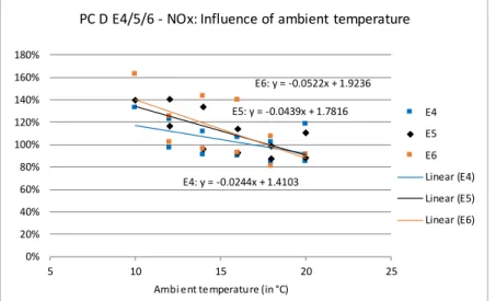
To analyse the ambient temperature effect on NOx isolated from mentioned influences, separate engine emission maps with RDE data measured at different ambient temperatures were created by PHEM using the CO2 interpolation method. Measured trips in similar ambient temperature ranges were summarized in one map, e.g. measured trips with veh_5 at 19 °C and 21 °C results in an engine emission map at 20 °C for veh_5. With these maps for the different temperature ranges, the CADC was simulated for each vehicle with PHEM. By simulating a common cycle from all emission maps the effects of different engine load cycles is eliminated and the results provide a common basis for the analysis of temperature influences on emissions. Since the CADC is representative for real world driving as mentioned before, the result for the temperature effects shall also be valid for real emission behaviour. Figure 11 shows the result of NOx emissions found with this method as function of ambient temperature. The trend is well described by a linear equation. The NOx emissions increase from 20 °C to 10 °C by approximately 40 % to 50 %. This high influence was the reason for further investigations based on remote sensing to validate the effects for the vehicle fleet and also to check temperature effects for older EURO classes. Finally, similar effects were found for EURO 4 to EURO 6 in the remote sensing data (Figure 12) and correction functions were implemented in HBEFA 3.3.
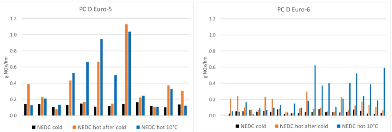
The following chart shows effects for EURO 4, EURO 5 and EURO 6 diesel cars. In addition the TUG data from the vehicle tests shown above are plotted (black rhombi), which fit the remote sensing data very well. As mentioned before, the EGR is optimised for a temperature range > 20 °C, therefore only data points are plotted below this threshold.
Figure 12: Preliminary NOx correction functions for EURO 4, EURO 5 and EURO 6 diesel cars based on vehicle tests and on remote sensing data from Sweden.
These linear equations from remote sensing measurement data were used as basis for the correction in the HBEFA but have been further adjusted to remote sensing data provided from tests in Switzerland.
The final correction functions were elaborated for the following boundary conditions:
Ambient temperature effect on NOx emissions occurs only below 20 °C for EURO 4, EURO 5 and EURO 6.
Ambient temperature effect on NOx emissions for EURO 6d-Temp and for EURO 6d are limited by the boundary conditions defined in the RDE regulation (limits have to be met down to 3 °C for EURO 6d-Temp and down to -3 °C for EURO 6d). Therefore, it is assumed for the future diesel vehicles that temperature effects are relevant only below these temperature thresholds.
NOx does not further increase below 0 °C. The available data do not cover lower temperatures, thus no statement on the real behaviour is possible at the moment. It is assumed, that EGR is on fleet average already reduced down to almost 0 % at 0 °C, so that no further effect on NOx occurs.
More details about the implementation of the temperature function are described in the final report for the HBEFA 3.3 (Keller M. et. al. 2017).
Effect of stop&go traffic on NO
xemissions for HBEFA 4.1
The emission factors for diesel passenger cars were simulated with PHEM in the past based on EoT emission maps, i.e. the emissions measured at end-of-tailpipe are binned into the engine map. In a cycle simulation then the emissions are interpolated from this map according to the simulated engine speed and power. PHEM offers also the simulation of the exhaust after-treatment system. Temperatures are simulated based on equations for heat transfer and energy conservation. The conversion efficiency of the catalysts can be modelled based on space velocity and temperature of the catalysts. Since the temperature of the catalysts changes rather slowly after load changes, the conversion efficiencies depend on a longer time span in front of the actual load point. Thus, the simulation of raw exhaust gas emissions and the conversion in the catalyst(s) may increase the accuracy especially in cycles where the catalysts leave the optimum temperature range. E.g. special traffic situations like stop&go traffic can result in relative high NOx levels due to low conversion efficiency resulting from cool down phases of the EAS if the engine has no special heating strategies. As disadvantage, the setup of the detailed EAS model for each vehicle increases the effort necessary to produce emission factors.
The actual EAS for diesel vehicles include an oxidation catalyst for CO and HC reduction as well as a filter for the particulates. For NOx reduction, a SCR catalyst or NSC or a combination of both is used. Due to the lambda (= air-fuel mixture ratio) 1 concept, for petrol vehicles only a 3-way catalyst is necessary. Some actual petrol cars use also a particulate filter.
To analyse the possible accuracy gains with a detailed EAS simulation for emission factors, one diesel EURO 6 car with oxidation catalyst, particulate filter, SCR catalyst and low plus high pressure EGR was investigated at TUG. The investigations for an EAS using NSC is still under investigation and the results will be used for the HBEFA 4.1 update. Based on these results it will be decided if also an investigation of EAS of petrol cars should be realised.
Table 4: Diesel EURO 6 measurements used for stop&go investigations.
ID Segment Odometer [km] Rated engine power [kW] Measurement at ambient temperature
Veh_I D-Segment 1000 90 36 °C
SCR catalyst is using NH3 to reduce NOx to N2 and H2O. NH3 is generated from AdBlue above approximately 200 °C by thermolysis and hydrolyses in the EAS. As shown in Figure 13, the NOx reduction in a SCR catalyst is mainly a function of the temperature, which results in lower conversion efficiency for lower temperatures. The curve is only valid, if enough NH3 for the NOx reduction is stored in the SCR catalyst (Hausberger S., Sams T. 2016).
Figure 13: NOx conversion rate as function of temperature (Hausberger S., Sams T. 2016). In the following, the effect of stop&go traffic on NOx emissions is presented with focus on:
Engine heating strategies: Investigation if the vehicle has an engine heating strategy in special driving situation to prevent low conversion efficiency resulting from cool down phases.
NH3 storage in the SCR system: The SCR catalyst can store NH3 to reduce NOx emissions also in lower temperature ranges since below 200 °C no AdBlue is injected. The question is, over which time span the amount of NH3 stored in the SCR catalyst is sufficient for a stop&go cycle driven after an usual driving cycle.
Simulation considering the EAS: Check if a simulation of engine heating strategies and of NH3 storage in SCR catalyst have to be implemented in the model PHEM for a sufficient accuracy. Compare the simulation accuracy with and without detailed EAS simulation. The stop&go cycle was driven at a flat test track to have repeatable boundary conditions for the measurements. The cycle was derived from real stop&go traffic and consists of an acceleration, steady-state driving at 8 km/h, deceleration to stand still followed by a 20 s stop.
Figure 14: Defined driving profile for stop&go traffic.
Figure 15: Defined accelerations for stop&go traffic.
The stop&go driving profile, shown in Figure 14, was driven in repetition for a duration of 27 minutes. The accelerations are between -1 m/s² to 1 m/s² (Figure 15).
Figure 16 shows the measured temperature (grey line) before SCR catalyst. It can be noticed, that the start temperature is between 250 °C and 300 °C since the vehicle was preconditioned at 80 km/h for several minutes to ensure repeatable conditions.
The measured temperature shown in Figure 16 settle down to approximately 170 °C. The trend shows no engine heating strategy at least for the first 1600 s. In the same figure is also the simulated temperature before SCR catalyst plotted (dotted black line), which also verifies the assumption that no heating strategy in the investigated time window exists since the simulation does not consider heating strategies so far.
Figure 17 shows the cumulated NOx over time. The grey line represent the measured NOx EoT, the dotted black line the simulated NOx considering the EAS in PHEM. For after-treatment simulation, PHEM uses an engine-out emission map and conversion maps for the EAS. E.g. the SCR catalyst is described with a map, where the conversion efficiency is a function of space velocity and temperature before SCR catalyst. Therefore, the exhaust gas mass flow and engine out temperature have to be provided in the engine maps as input for PHEM. The mass flow and temperature maps can be derived from measurement data. The NOx conversion map can also be derived from measurement data, if the concentration of NOx upstream and downstream, the exhaust gas mass flow through the SCR catalyst and the temperature before SCR catalyst are available for each time step. For the investigated vehicle, all mentioned measurement data of several RDE and stop&go trips were used to produce emission and catalyst maps.
The simulated NOx (dotted black line in Figure 17) using the after-treatment simulation in PHEM mostly fit the measured NOx level. After 1600 s the measured NOx level is at 233 mg/km, the simulation with after-treatment system leads to a 1 % lower NOx level. In the same figure also a black line is plotted, showing the simulation result using the simple EoT map. For the EoT map the emissions measured end-of-tailpipe during the same trips used for after-treatment simulation (i.e. all measured RDE and stop&go cycles) are sorted in an engine map according to the engine power and engine speed using the CO2 interpolation method. This map includes the EAS indirectly in the emission behaviour. The simulation without considering after-treatment system can lead to higher deviations between simulation and measurement. In this case the deviations results in 5 % lower NOx after 1600 s. The time resolution is much better with the detailed EAS model since the simple EoT map is representing average temperature conditions and cannot show cool down effects.
On the other side, simulations by EoT maps are easier and faster since no EAS calibration and simulation in PHEM is necessary. The good agreement between the measurement data and the simulated data considering the EAS assume that the NH3 storage in the SCR catalyst is sufficient since PHEM cannot consider the NH3 storage so far. This assumption was also checked with a developed NH3 storage model, which can be used currently as a post-processing application after measurement and/ or PHEM simulation. The model confirms that for the investigated stop&go cycle sufficient NH3 is available, if the SCR catalyst was filled with 50 % of maximum possible NH3 at the beginning of the test cycle. The NH3 storage model will be presented in detail in the HBEFA 4.1 report.
Figure 16: Measured and simulated
temperature of stop&go cycle. Figure 17: Measured and simulated NOx of stop&go cycle.
Conclusion and outlook
For the HBEFA version 3.3 the new CO2 interpolation method was used to produce the engine emission maps. With this method, it is possible to consider also measurement data where the engine load signal is not available or too inaccurate for engine map creation. This is especially useful for RDE measurements, where the power signal in most of the cases is not available. Using RDE measurements beside the chassis dynamometer test data increase the sample size of tested vehicles and improves in general the representativeness of the engine emission maps. In total the measurement data of 25 diesel EURO 6 cars were used for the update. Since the HBEFA 3.3 is a so-called quick update, only the NOx emissions of diesel EURO 6 vehicles were updated. Based on the NOx emissions for diesel EURO 6 vehicles also an assumption for diesel EURO 6d-Temp and EURO 6d vehicles considering the RDE conformity factor was done since no such vehicles were available so far for measurements. The RDE legislation prescribes a conformity factor of 2.1 for EURO 6d-Temp and of 1.5 for EURO 6d. This means that for a valid RDE trip, the NOx shall not be higher than the NOx emission limit on WLTC multiplied by 2.1 for EURO 6d-Temp, which results in 168 mg/km, and not be higher than 120 mg/km for EURO 6d. Since the RDE legislation covers a large range of driving conditions and includes also PEMS tests from independent parties, it is assumed that vehicles will meet the standards in “normal” real world cycles of HBEFA but not in stop&go and under high gradients. Consequently, the simulated NOx emission factors decrease for the new emission standards by approximately 50 % to 70 % without considering the ambient temperature effect.
With the extended sample on measurement data due to additional RDE trips, also investigations like ambient temperature influence on NOx emissions were realised. The measurement data of several conventional diesel EURO 6 cars at different ambient temperatures were used. To analyse the ambient temperature effect on NOx isolated from routes and driving behaviour, separate engine emission maps with RDE measurement data at different temperatures were created and a standard CADC cycle was simulated with these maps. The investigation showed that from 20 °C to 10 °C ambient temperature the NOx increase by approximately 40 % to 50 % for a real world cycle. This was the basis for consideration of ambient temperature effect on NOx emissions in HBEFA 3.3.
Also an investigation regarding the effect of stop&go traffic on NOx emissions was performed. The goal was to investigate if a detailed EAS simulation should be used in PHEM for the HBEFA 4.1 update. The simple tailpipe emission map meets the average NOx in g/km quite accurately, but the second-by-second NOx trend is much better if the EAS is considered in the simulation. The handling for HBEFA 4.1 is still open, further investigations are ongoing.
Acknowledgments
The HBEFA 3.3 quick update would not have been possible without the support from vehicle emission labs: EMPA (Switzerland), TNO (Netherlands) and ADAC (Germany), which provided chassis dynamometer and RDE measurement data. IVL (Sweden) and AWEL (Switzerland) also provided remote sensing data to consider the ambient temperature effects on NOx emissions. The authors would furthermore like to thank Mario Keller (INFRAS / MK Consulting, Switzerland) for the ERMES DB management and for processing of the simulated emission factors.
Finally, the work would not have been possible without the funding from UBA Germany and UBA Austria, who set up projects as basis for the HBEFA quick update and for the HBEFA 4.1 update.
References
Hausberger S., Ligterink N., et.al.: Correction algorithms for WLTP chassis dynamometer and coast-down testing; report for DG Enterprise; TNO, Netherlands, 2015
Hausberger S., Matzer C.: Update of Emission Factors for EURO 4, EURO 5 and EURO 6 Diesel Passenger Cars for the HBEFA Version 3.3, Graz, 01. June 2017
Hausberger S., Rexeis M., Zallinger M., Luz R.: Emission Factors from the Model PHEM for the HBEFA Version 3. Report Nr. I-20/2009 Haus-Em 33/08/679 from 07. December 2009
Hausberger S., Sams T.: Schadstoffbildung und Emissionsminimierung bei Kfz Teil I und II, Skriptum IVT TU Graz, Graz, 2016
Hausberger S., Stadlhofer W., Vermeulen R., Geivanidis S., et.al.: MAC performance test procedure; Co-ordination of the pilot test phase and follow up towards the drafting of the regulatory text; Performed under Framework Service Contract ENTR/05/18, European Commission - DG Enterprise and Industry; April 2013 Hill N., Windisch E., Hausberger S., Matzer C., Skinner I., et.al.: Improving understanding of technology and costs for CO2 reductions from cars and LCVs in the period to 2030 and development of cost curves; Service Request 4 to LDV Emissions Framework Contract; Final Report for DG Climate Action; Ref. CLIMA.C.2/FRA/2012/0006; Ricardo AEA, UK, 2015
Keller M., Hausberger S., Matzer C., Wüthrich P., Notter B.: HBEFA Version 3.3, Background documentation, Berne, 12. April 2017
Luz R., Hausberger S.: User Guide for the Model PHEM, Version 10; Institute for Internal Combustion Engines and Thermodynamics TU Graz, Graz, 2009
Matzer C., Hausberger S., Lipp S., Rexeis M.: A new approach for systematic use of PEMS data in emission simulation, 21st International Transport and Air Pollution Conference, Lyon 24. – 26. May 2016
Rexeis M.: Ascertainment of Real World Emissions of Heavy Duty Vehicles. Dissertation, Institute for Internal Combustion Engines and Thermodynamics, Graz University of Technology. October 2009
Zallinger M.: Mikroskopische Simulation der Emissionen von Personenkraftfahrzeugen. Dissertation, Institut für Verbrennungskraftmaschinen und Thermodynamik, TU Graz, Graz, April 2010
Variations of Real-world NOx Emissions of Diesel Light Commercial
Vehicles
Gerrit Kadijk*, Veerle A.M. Heijne, Norbert E. Ligterink, Robin J. Vermeulen.
Research Group Sustainable Transport and Logistics, TNO, PO Box 96800, 2509 JE Den Haag, the Netherlands, correspondence: gerrit.kadijk@tno.nl, presenter: veerle.heijne@tno.nl
Abstract
In order to gain insight into trends in real-world emissions of diesel light commercial vehicles under conditions relevant for the Dutch and European situations, fifteen Euro 6/VI and three Euro 5 light commercial vehicles (LCVs) were extensively tested on the road during the spring and summer of 2017. These measurements form the basis of the annual update of Dutch emission factors. On the road, real-world NOx emissions of Euro 6/VI LCVs range from 30 to 1400 mg/km,
on average 1 to 5 times higher than the type approval limit value. The measured average NOx
emission of the Euro 6/VI commercial vehicles in the test programs varies between 60 and 505 mg/km. In general, the difference between real-world emissions and type approval emission limit values has been growing over the years, but this trend seems reversed now with Euro6/VI LCV vehicles. For future diesel vehicles, an improvement of real-world NOx emissions is expected with
Real Driving Emission legislation. Currently the relatively expensive PEMS is foreseen as the type approval standard for on-road testing. TNO also applies a NOx-O2 sensor-based system with data
logger (SEMS) as a NOx screening tool.
Key-words: Real-world NOx emissions, light commercial vehicles, Euro 6, Euro VI, RDE, SEMS
Introduction
Commissioned by the Dutch Ministry of Infrastructure and the Environment, TNO regularly performs test programs to determine the real-world emission performance of vehicles in the Netherlands (Kadijk et al., 2015 a,b,c & 2016 a,b,c & 2017) and (Spreen et al., 2016). The main goal of the programs is to gain insight into trends in real-world emissions of light- and heavy-duty vehicles under conditions relevant to the Dutch and European traffic situations. In 2016 and 2017 in total eighteen vehicles were tested: three Euro 5 light commercial vehicles, two Euro 6 passenger cars and thirteen Euro 6/VI light commercial vehicles (LCVs).
Based on the performed emission measurements, TNO develops and annually updates vehicle emission factors that represent real-world emission data for various vehicle types and different driving conditions. Vehicle emission factors are used for the Dutch emission inventory and air quality monitoring. TNO is one of the few institutes in Europe that perform independent emission tests for real-world conditions. Dutch emission factors are nowadays based on these on-road tests. The emission factors are one of the few independent sources of information on the growing difference between legislative emission limits and real-world emission performance of cars. To minimize air pollutant emissions of light-duty vehicles, in 1992 the European Commission introduced the so-called Euro emission standards. Over the course of time, these standards have become more stringent. Since September 2014, all new type approved N1 Class 1 light-duty vehicles must comply with Euro 6 regulations and from September 2015 onwards all registered vehicles need to comply with the Euro 6 limits, therefore the tested vehicles are relatively early models. For the N1 Class 2 and 3 vehicles these dates are valid a year later. The standards apply to vehicles with spark ignition engines and to vehicles with compression ignition engines and cover the following gaseous and particulate emissions: CO (carbon monoxide), THC (total hydrocarbons), NOx (nitrogen oxides), PM (particulate mass) and PN (particulate number). The focus of the test program was on compression ignition (diesel) vehicles.
As a result of the Euro emission standards, the pollutant emissions of light-duty vehicles as observed in type approval tests have been reduced significantly over the past decade. However, under real driving conditions, some emissions substantially deviate from their type approval equivalents. The real-driving nitrogen oxides, or NOx, emissions of diesel vehicles are currently the largest issue with regard to pollutant emissions. As NOx represents the sum of NO and NO2
emitted, reducing NOx emissions of vehicles is an important measure in lowering the ambient NO2 concentration. In the Netherlands, the ambient NO2 concentration still exceeds European limits at numerous road-side locations.
TNO regularly performs emission measurements within the “in-use compliance program for light-duty vehicles” and the “in-use compliance program for heavy-light-duty vehicles”. Whereas in the early years, i.e. in 1987 to 2000, many standard type approval tests were executed, in recent years the emphasis has shifted towards the gathering of real-world emission data. Real-world emission data are collected by means of:
1. Performing emission measurements on a chassis dynamometer using various non-standard driving cycles, for example driving cycles that better reflect real-world driving conditions, and; 2. Equipping vehicles with an on-board emission measurement system (PEMS and/or SEMS) to measure the emissions of the vehicles while driving on the public road.
In the Netherlands, the road tax and fuel excise duty system discourages the private ownership of diesel cars. Only 15% of the passenger cars are diesel in the Netherlands. With 8 million passenger cars, the 900,000 LCVs in the Netherlands are not negligible, since there are almost as many diesel LCVs as diesel passenger cars in the Netherlands. These LCVs are responsible for about half of the total NOx emission of light-duty vehicles. According to the revenue office, most of the LCVs are associated with some commercial use. However, especially older vans are also used extensively in the evening and the weekend. Very likely the Euro 5 and Euro 6 LCV will be an important contributor to urban ambient NO2 concentrations in 2020 and beyond.
Objective
The objective of this research is to assess the real-world emission performance of Euro 6/VI light commercial vehicles. For three vehicle types from the N1 Class 3 category, Euro 5 variants were tested as well.
Method
On-road testing
Emission tests were performed on the road. TNO performs real-world tests on the road with a Portable Emission Measurement System (PEMS) and/or a Smart Emission Measurement System (SEMS). PEMS equipment measures CO, CO2, HC, NO and NO2 emissions. SEMS is an emission screening tool which contains a data logger and a NOx-O2 sensor. Moreover, with SEMS NH3 emissions are monitored. In this test program, all emission tests were performed with SEMS. SEMS testing
Emission tests with different vehicles were performed on the road under real-world conditions. During the SEMS tests, the vehicle was loaded with a test driver, additional payload and the test equipment with a weight of approximately 5 kg.
In recent years, TNO has developed the so-called Smart Emission Measurement System or SEMS (Vermeulen et al. 2012 & 2014). SEMS is an emission screening tool that contains a data logger, a NOx-O2 sensor (Continental, UniNOx) and a thermocouple temperature sensor, of which the latter two are installed in the tailpipe of the vehicle. It measures the exhaust gas temperature and the O2 and NOx volume concentrations in vol% or ppm. SEMS also measures geographical data, vehicle speed and logs the CAN data of the vehicle with a measuring frequency of 1 Hz. Based on the measured O2 readings and the carbon and hydrogen content of the fuel, the CO2 concentrations are calculated. In former projects, the accuracy and the reliability of the SEMS equipment and method has been demonstrated (2012), (2014b).
In this test program the data of the MAF (Mass Air Flow) sensor of most of the tested vehicles was used for the calculation of the NOx and CO2 exhaust mass flow rates [mg/km]. The quality of the air mass rate signal of the vehicle has a large influence on the accuracy of the NOx and CO2
mass emissions. Moreover, the NOx-O2 sensor is sensitive for temperature and pressure which may influence the accuracy. Calibration of the MAF sensor and the NOx-O2 sensor is a standard part of the test procedure.
The test and data processing procedure contains the following steps:
1. Before and after every test session the fuel tank of the vehicle is filled off at the same pump of the same filling station;
2. The measured mass air flow rate from the vehicle, the measured NOx and O2 concentrations are corrected based on calibration data;
3. The CO2 volume concentration is determined from the measured O2 volume concentration and the fuel C:H ratio;
4. The exhaust mass flow rate is determined from the vehicle Mass Air Flow signal, augmented with combustion products CO2 and H2O using the fuel C:H ratio and the normal air density. In case no Mass Air Flow signal is available, the exhaust mass flow rate is estimated using the fuel flow rate and the measured oxygen concentration; 5. The CO2 and NOx mass flow rates are determined from the measured volume
concentrations and the exhaust mass flow rate. This analysis requires three input parameters:
- the C:H ratio of the fuel, which is assumed to be 1.95 for modern market-fuel diesel; - the ambient oxygen content of air at 20.8% for on-road conditions;
- normal air density of 1.29 kg/m3 at standard conditions to calculate the exhaust gas density.
Performance of SEMS test equipment on a chassis dynamometer
The NOx-O2 sensors of the SEMS equipment and the mass air flow (MAF) sensors of most vehicles are calibrated. Independent verification with data of refills was used to determine the quality of the air flow signal of the different vehicles. The total CO2 emissions between refills, as determined from the fuel and from the air flow signal was equal for all vehicles, within a 5% range. No systematic deviation from this 5% variation was found. It was noted that at very low concentrations of NOx, the SEMS sensor is less accurate for transient signals. However, in the range of concentrations of the current measurements the correlation and calibration tests carried out in the last four years provide a good evidence for the accuracy of the measurements (Spreen et al., 2016b).
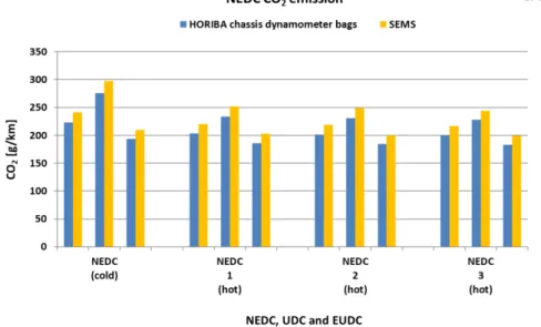
Figure 1: Example of validation CO2 test results SEMS-chassis dynamometer of one vehicle (per test the total result and urban and extra-urban results are shown).
In order to validate the SEMS test results, over the last three years validation tests with four vehicles were performed on a chassis dynamometer. The CO2 and NOx test results of one vehicle are shown in Figure 1 and Figure 2. The SEMS test results are well in line with the chassis dynamometer test results. SEMS test results are partly based on (corrected) MAF data of the CAN-bus of the vehicle. In all emission tests the difference of the CO2 emissions is 8% and the difference of the NOx emissions is -14% to +12%. Both standard deviations for CO2 are approximately 1%; for NOx, these equal 8 and 12%. The results show that SEMS is a useful screening tool which yields repetitive indicative results. One should keep in mind that the accuracy of these test results is directly related to the accuracy, resolution and response time of the mass air flow signal of this vehicle type. Other vehicle types may gain different accuracies.
Although SEMS is less accurate than PEMS, the system is well suited for a quick screening of NOx emissions of a vehicle and for measuring and monitoring over long periods of time. Its error margins are sufficiently low to identify emissions that are well beyond emission limits.
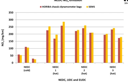
Figure 2: Example of validation NOx test results SEMS-chassis dynamometer of one vehicle (per test the total result and urban and extra-urban results are shown).
Test routes
SEMS registers real-world conditions and real-world emissions. To be able to compare the individual real-world vehicle emissions, one Real Driving Emission (RDE) trip (with 28% payload and a hot start), an in-service conformity trip (ISC) and a delivery trip are always part of the investigation. The RDE and ISC trips consist of urban, rural and highway driving. Additionally, some other trips are driven: RDE trips with a cold start, a trip mainly containing urban driving and a trip consisting mainly of highway driving. Table 1 shows the main characteristics of the test trips. All trips start in Delft or The Hague, the Netherlands. Tests are carried out with different payloads and different driving styles.
Table 1: Specifications of SEMS test trips.
Trip Name Road Type(s) Start condition Driving style Test Day Payload [%] Distance [km] Average velocity [km/h]
1 RDE_C Urban / rural / motorway Cold start Economic 1 28 74.7 43
2 Motorway Motorway Hot start Regular 1 28 89.5 79
3 RDE_H Urban / rural / motorway Hot start Regular 1 28 74.7 43
4 Congest_W Motorway, evening traffic Hot start Regular 1 28 84.3 56
5 Congest_C Motorway, morning traffic Cold start Dynamic 2 95 85.3 83
6 City Urban Hot start Regular 2 95 27.8 21
7 Rural Rural Hot start Regular 2 95 64.5 50
8 RDE_H Urban / rural / motorway Hot start Regular 2 95 74.7 43
9 City to City Urban / rural / motorway Hot start Regular 2 95 21.2 36
10 RDE_C Urban / rural / motorway Cold start Regular 3 55 74.7 43
11 Short trip Urban/rural Hot start Regular 3 55 4.3 28
12 Delivery trip Urban Hot start Regular 3 55 17.4 12
13 ISC_H Urban / rural / motorway Hot start Regular 3 55 122.7 57
14 City to City Urban / rural / motorway Hot start Regular 3 55 21.2 36
Total 837.1
Table 2: Driver instructions of different driving styles.
Driving style Economy Normal Sportive
Driving behaviour careful regular dynamic
Gearshift engine speed [rpm] 2000 2500 3500
Distance to target at start of braking [m] 90 60 30
Delay time speed to brake pedal [s] 30 3 0
Start-stop system active Yes Yes No
Vehicle stops of 120-180 s 0 0 2
Maximum position speed pedal [%] 80 90 100
Speed pedal activation speed slow normal fast
Maximum speed on the motorway [km/h] 110 120 140
Driving styles in on-road measurements
The test driver is given instructions for three different driving styles: ‘economic’, ‘normal/regular’ or ‘dynamic/sportive’. Some vehicles are tested with all driving styles. In Table 2 more details of the driving styles are reported.
Test vehicles
Table 3 shows the eighteen tested Euro 5, 6, and VI vehicles in the measurement program. The two M1 vehicles can be considered as N1 class 3 vehicles because they both have similar engines and aftertreatment technologies.
Table 3: Tested Euro 5, 6 and VI vehicles in 2016 and 2017.
Brand Model Category Euro
Class Power [kW] Aftertreatment Odometer [km] Mass empty [kg]
Peugeot Partner N1 class 2 6b 73 Oxicat+DPF+SCR 21,263 1,460
Renault Trafic N1 class 3 6b 92 Oxicat+DPF+SCR 3,200 2,065
Ford Transit
Connect N1 class 2 6b 74 Oxicat+DPF+LNT+SCR 15,353 1,596
Volkswagen Caddy N1 class 2 6b 55 Oxicat+DPF+SCR 4,498 1,486
Volkswagen Kombi
Transporter M1 6b 62 Oxicat+DPF+SCR 20,004 1,894
Mercedes-Benz Citan N1 class 2 6b 55 Oxicat+DPF+LNT 17 1,448
Mercedes-Benz Vito M1 6b 100 Oxicat+DPF+SCR 44,875 2,477
Peugeot Expert N1 class 3 6b 90 Oxicat+DPF+SCR 12,878 1,817
Ford Transit N1 class 3 5b 74 Oxicat+DPF 56,356 2,167
Ford Transit N1 class 3 6b 96 Oxicat+DPF+SCR 11,751 2,383
Ford Transit N1 class 3 VI 114 Oxicat+DPF+SCR 37152 3181
Mercedes-Benz Sprinter N1 class 3 5b 95 Oxicat+DPF 23,878 2,535
Mercedes-Benz Sprinter N1 class 3 6b 105 Oxicat+DPF+SCR 12,770 2,695
Mercedes-Benz Sprinter N1 class 3 VI 120 Oxicat+DPF+SCR 30,734 2,960
Volkswagen Crafter N1 class 3 5b 100 Oxicat+DPF 60,544 2,146
Volkswagen Crafter N1 class 3 6b 80 Oxicat+DPF+SCR 2,694 2,158
Volkswagen Crafter N1 class 3 VI 120 Oxicat+DPF+SCR 70,780 2,146
Iveco New Daily N1 class 3 6b 114 Oxicat+DPF+SCR 4,488 2,366
Results
All eighteen vehicles were tested on the road with SEMS. Emission and vehicle data were logged in 132 defined tests with a total distance of more than 9000 km with a measuring frequency of 1 Hz. The names of the specific trademarks and vehicle types are not mentioned in the results. These will be given in a TNO report, which is expected to be published before the end of 2017. Overview NOx emissions of Euro 6/VI vehicles:
Figure 3 shows the large spread in the average NOx emissions of the executed test trips of all fifteen Euro 6/VI LCVs. A typical RDE test has an average speed of 35 – 45 km/h and average NOx emissions in the range of 39 - 534 mg/km. Other trips with this average speed yield higher emissions (up to 1050 mg/km). The NOx emissions in urban traffic (around an average speed of 15 km/h) are in the range of 100 – 1300 mg/km. One N1 class 2 vehicle with an LNT has in short urban trips of 4-5 km the highest urban NOx emission around 1300 mg/km. The lowest average NOx emissions, in the range of 50 – 500 mg/km, were measured in trips with higher average vehicle speeds (60 – 85 km/h).
Figure 3: Average on-road NOx emissions of different test trips with different payloads and different driving styles of fifteen Euro 6/VI light commercial vehicles.
Detailed NOx emissions of Euro 5/6/VI vehicles:
More specific variations of NOx emissions of the Euro 5/6/VI vehicles are shown in Figure 4 up to Figure 7. In this test program the bandwidth of the average NOx emissions of the fifteen Euro 6/VI vehicles is 60 – 514 mg/km and the bandwidth of the average NOx emissions of the three Euro 5 vehicles is 648 – 1498. The latter are in line with earlier TNO findings (Kadijk 2015a). The average NOx emissions of the Euro 6/VI LCVs are substantially lower than the Euro 5 variants.
The NOx emissions of Euro 6/VI vehicles in RDE tests, see Figure 4, are in the range of 36 to 534 mg/km and they have no direct relationship with the size of these vehicles. The performance of the applied emission control systems seems to be more decisive for the NOx emissions.
The RDE test results of all vehicles in Figure 4 clearly show that the CO2 emission of the vehicles is not related to the NOx emission. The best comparison can be made with the vehicles J, K and L, which were all tested in a Euro 5, 6 and VI variant. The CO2 emissions of each type are in a comparable range (+/- 10%) but their NOx emissions vary with a factor 6 – 28 (600 – 2800%). Vehicle A (N1 class 2) and vehicle E (N1 class 3) already meet the Euro 6d RDE NOx limit value in certain RDE tests with moderate conditions.
The NOx emissions of fourteen Euro 6/VI vehicles in RDE trips with 28% payload are 36 – 534 mg/km and the NOx emissions of HD-ISC trips with 55% payload are 38 – 448 mg/km, see Figure 4 and Figure 5. Three Euro 6/VI vehicles emit in HD-ISC tests more NOx than in RDE tests, eight vehicles have substantially lower NOx emissions and three vehicles have a similar performance in both tests.
The NOx emissions in delivery trips (see Figure 6) of these fourteen Euro 6/VI vehicles are in the range of 128 – 838 mg/km and are on average substantially higher than the NOx emissions in RDE & HD-ISC tests (36 – 534 mg/km).
Figure 4: Average on-road NOx and CO2 emissions of RDE test trips of fifteen Euro 6/VI and three Euro 5 light commercial vehicles.
Figure 5: Average on-road NOx and CO2 emissions of HD-ISC test trips of fifteen Euro 6/VI and three Euro 5 light commercial vehicles.
Figure 6: Average on-road NOx and CO2 emissions of delivery test trips of fifteen Euro 6/VI and three Euro 5 light commercial vehicles.
In Figure 7 the total average NOx emissions of the executed test programs of all eighteen vehicles are shown. For the Euro 6/VI vehicles J, K and L the total average NOx emissions are 60 – 560 mg/km, which is substantially lower than the total average NOx emissions (648 – 1498 mg/km) of the Euro 5 variants of these types.
Figure 7: Average on-road NOx and CO2 emissions of all trips of fifteen Euro 6/VI and three Euro 5 light commercial vehicles.
The effects of different payloads and driving styles:
In Figure 8 and Figure 9 the CO2 and NOx results of RDE tests of eight vehicles are shown. Variations were set in payloads (28%, 55% and 95%) and three different driving styles were executed (economic, normal and sportive). The main target of these variations was to cover the whole RDE operating range with respect to payload, driving style and vehicle speeds. Since the driver instructions in terms of driving style and maximum vehicle speeds were restricted due to traffic situations, the actual execution of the RDE test may deviate.
Figure 8: CO2 emissions of RDE test trips with different payloads, driving styles and starting conditions of eight Euro 6 light commercial vehicles.