Field uniformity and isotropy investigation of Halmstad University's reverberation chamber: In collaboration with Halmstad University and Ericsson AB, Lund

Master Thesis

HALMSTAD

UNIVERSITY

Master's Programme in Electronic's Design, 60 credits

Field uniformity and isotropy investigation of

Halmstad University's reverberation

chamber

In collaboration with Halmstad University and Ericsson

AB, Lund

Master Thesis 15 credits

Halmstad 2020-06-05

Khaled Ads

- 1 -

Abstract

This thesis is the final module of the Master's program in Electronics Design at Halmstad University.

The Master Thesis work is a part of an ongoing development of Halmstad University's reverberation chamber (RC), which is aimed at frequencies in the low GHz range. The development process has been passing in several phases. One phase is to design a mechanical stirrer system which was done by the work presented in another thesis work. The current phase, which is done by this thesis work, is to investigate electromagnetic field uniformity and isotropy while using tuned-mode (stepped stirrer). The frequency 2.4 GHz was chosen because, from one hand, it fits the capability of the assigned equipment for this thesis (spectrum analyzer, signal generator, antennas). On the other hand, it is the operating frequency of a wide range of WIFI and Blue-Tooth devices that need to be tested inside the RC to comply with the Electromagnetic Compatibility (EMC) standards. The measurement results verified, to a reasonable extent, the field uniformity and isotropy. The standard deviation of all measurements, taken from different eight positions with three different orientations of the receiving antenna, was 1.5dB. It is less than 3dB fulfilling the IEC 61000-4-21standards for frequencies above 400MGHz. Moreover, a quality factor degradation test was conducted, showing a 3.5 dB reduction of the received power when the chamber was loaded by organic material. The received power, while sweeping the bandwidth 800MHz-1.5GHz, was measured. These results indicate that at the resonance frequencies of the chamber, the received power is higher than that at non-resonance frequencies.

Foreword

I would like to thank everyone who helped or supported me during this thesis work. The work would not have been completed without their support. Thanks to Stefan Nilsson, the supervisor, for his appreciated guidance and supervision. Thanks to Peo Karlsson for providing me with all the required facilities. Last but not least, thanks to Pererik Andreasson for his valuable tips about how to make my thesis writing professional and how to perform the work in a scientific manner. Last but not least, a big thanks to the Swedish Institute (SI) for granting my scholarship and giving me this valuable opportunity to complete my Master’s degree.

- 2 -

- 3 -

Contents

1 introduction

……….…….…...………… 5 1.1 Historical view ……….…….. 5 1.2 Theory of operation ………. 5 1.2.1 Standing wave ……….……… 5

1.2.2 Transverse Electric and transverse Magnetic modes ………..…..6

1.3 Operating parameters ……….……..…...5

1.3.1 Resonance frequency and number of modes………..…….………7

1.3.2 Chamber Quality factor (Q) ……….……...8

1.4 RC physical description ……….…... 10

1.5 RC applications ……….………..….. 10

1.6 Reverberation chamber versus Anechoic Chamber ………..…………..……….…. 11

1.7 Antenna principles ………..…... 12

1.7.1 Radiation Pattern ………..……….…...…. 12

1.7.2 Antenna Directivity, Gain, and Efficiency ………....…….13

1.7.3 Antenna polarization ………...……13

1.8 Spectrum analyzer theory of operation ………..……….…..14

1.8.1 Applications of a spectrum analyzer ………...14

1.8.2 Spectrum analyzer function block diagram description ………..………….15

1.8.3 Resolution bandwidth and phase noise ……….……17

1.9 Transmission Line ………19

2 Methodology

………...19

2.1 Instruments and software ………..……...19

2.1.1 Signal generator (Ana-Pico APGEN 3000) ……….19

2.1.2 Spectrum analyzer Rohde & Schwarz R&S FPC 1000 ...20

- 4 - 2.1.4 Receiving (Rx) antenna ………...………20 2.1.5 Stirrer system ………...20 2.1.6 Software ………..……20 2.1.6.1 Python-Visa ………..20 2.1.6.2 SCPI ………..21 2.2 calculations ……….…...21

2.2.1 Lowest Usable Frequency (LUF) ……….………21

2.2.2 Working volume ………..………..….…..22

2.3 Field uniformity validation ………..…..22

2.3.1 Variance and Standard Deviation ……….….24

2.3.2 Test set up ……….….24

2.3.3 Measurements results ………..…...26

2.3.4 Sweeping measurements ………..….….28

2.3.5 Quality factor degradation test ………...29

3 Discussion

………..………..…33

3.1 Field uniformity and isotropy ……….33

3.2 Sweeping measurements ………....34

3.3 Quality factor degradation test ………..……37

4 conclusion

……….……39

5 Recommendations for continued work

………..………..……39

References

………..……41

Acronyms .

………..43

Appendix ………..……

44

- 5 -

1. Introduction

The work starts with presenting the theory of operation for the RC and the used equipment in the measurement process (spectrum analyzer, antenna, transmission line). The methodology section presents the test set up, the Python code used to control the measurement instrument, and all measurements. The outcome of measurement results is discussed in detail in the discussion section. A conclusion is listed in the conclusion section. A new environmental test is proposed in the RC and the environment section. Finally, recommendations for further future work on the RC are listed.

1.1 Historical view

By the last decade of the twentieth century (the 1990s), the need for measuring Electromagnetic Compatibility (EMC) and Electromagnetic Interference (EMI) tests had to cope with the crowd of an enormous different kind of electronic equipment. It is an inevitable task to make sure that any manufactured electrical equipment or electronic device fulfills EMC and EMI tests. The mutual effect of electrical devices from the electromagnetic radiation perspective plays a crucial role in their performance. It is essential to optimize their electromagnetic radiation in terms of frequency and power. Fulfilling EMC secure that the electrical devices can operate normally without affecting severely other electrical devices sharing the same environment[1]. On the other hand, it ensures that their performance will not be degraded by the EMI from the neighboring devices. As wireless communication technology has been evolving exponentially over the last three decades in terms of transmitting and receiving apparatus, the role of the reverberation chamber became remarkably crucial for the wireless industry. RC provides not only a feasible and practical measurement environment but also time-saving test procedures compared with its counterpart Anechoic Chamber (AC). In 1964 H.A. Mendes proposed for the first time RC as a new technique to measure the electromagnetic field strength[1]. So that the requirement of RC was increased and turned into a necessary means of performing EMC and EMI. In 2003 The International Electrotechnical Commission (IEC) conducted an international standard (IEC 61000-4-21) for using RC in the EMC measurement.[19] In 2001 professor Per-Simon Kildal (Chalmers University of Technology) was behind the first RC measurement system consisting of an RC chamber and software that was delivered to a large Asian mobile terminal manufacturer. That came after a decade of research to prove that reverberation chambers could be used for characterizing small antennas and mobile devices.[2]

1.2 Theory of operation

1.2.1 Standing wave [3]

As the incident wave inside the RC reflects from the conducting surfaces inside the chamber (walls, ceiling, floor, stirrer blades), the reflected wave interferes with the incident wave constructing a standing wave.

Standing wave pattern is determined by the mathematical summation of both the incident and reflected waves. So that the maximum value of the standing wave pattern corresponds to the position at which both the incident and the reflected wave are in phase (having 2nπ phase shift; n is an integer) and therefore add constructively figure(1.1). The minimum value of the standing wave pattern corresponds to the position at which both the incident and the reflected wave are in phase-opposition (having [2n+1] π phase shift; n is an integer) and therefore add destructively figure (1.2). If the amplitude of the reflected wave is less than that in

- 6 -

the incident wave, the resulting standing wave constructs an envelope with a repetition period of λ/2. Considering the incident and the reflected wave repetition period individually is λ (wavelength in meter), the repetition period of the standing wave is λ/2 this means that the maxima of the standing wave appear every half wavelength of the incident wave figure (1.3)

Figure (1.1) constructive interference Figure (1.2) destructive interference figure (1.3) standing wave

1.2.2 Transverse Electric and transverse Magnetic modes [3]

Transverse Electric Mode (TE): Considering the three orthogonal directions x, y, and z, when the electromagnetic wave (EM) propagates in the z-direction and the (z) component of the electric field vector is equal to zero. So that the electric field vector is always perpendicular to the direction of propagation (z). This mode of propagation is called the Transverse Electric mode (TE).

Transverse Magnetic Mode (TM): If the (z) component of the magnetic field vector is equal to zero, the magnetic field vector is always perpendicular to the direction of propagation (z). This mode of propagation is called the Transverse Magnetic mode (TE).

Transverse Electromagnetic Mode (TEM)

:

In TEM mode, the z-component of both the electric field and the magnetic field vectors are equal to zero. The electric field and magnetic field are propagating orthogonally to the direction of propagation. This mode needs a current source to exist; that is why it exists in coaxial cable carrying current but does not exist in a rectangular waveguide and RC. For a rectangular waveguide, if the direction of propagation is (z) while (x) and (y) are the width and the height respectively, the lowest mode of propagation TE10 means that there is one half of the wavelength λ in (x). TE20 means there are two halves of

the wavelength λ in (x), whereas TE01 means there is one half of the wavelength λ in (y), and TE20 means there

are two halves of the wavelength λ in (y). Figure (1.4) presents TE10&TE20&TE30 in x-y plane. Different TE

and TM modes are illustrated in figure (1.5)

- 7 -

Figure (1.5) Field lines for some of the lower order modes of a rectangular waveguide [4]

1.3 Operating parameters

1.3.1 Resonance frequency and number of modes

RC operates on the phenomenon of the cavity resonator in which several modes are created according to the RC dimensions and the exciting frequency inside the chamber. As the electromagnetic radiation inside the RC reflects from the ceiling, walls, and floor, moreover stirred by the mechanical stirrer, it causes the incident wave to interfere constructively with the reflected wave resulting in standing waves. Nevertheless, there is destructive interference which quenches the wave.

Figure (1.6) shows a 3-D simulation of modes inside RC (number of field peaks or half wavelengths) [1]

- 8 -

The resonance frequencies of the chamber can be calculated by the following equation (1.1) which is derived from solving Maxwell's equations[1]

(1.1)

Where m, n, p are the number of modes in x, y, z directions respectively m=0,1,2,3,… & n=0,1,2,3,… & p=0,1,2,3,… while a, b, d are the chamber dimensions in x, y, z in meter, and fmnp is the resonance frequency

in Hz, where μ, ε are the permeability and the permittivity of the medium inside the cavity, respectively.

Number of modes is given by Weyl's formula (1.2) for rectangular cavities[1]

𝑁 =

8𝜋 3

(𝑤. 𝑙. ℎ)

𝑓3 𝑐3

− (𝑤 + 𝑙 + ℎ)

𝑓 𝑐

+

1 2

(1.2)

Where 'c' is the speed of the electromagnetic wave inside the cavity, which equals to 3*108 m/s. and w,l,h are width, length, and height, respectively. Mode density also is an important parameter to be considered. It reflects how many modes available in a narrow bandwidth of a specific center frequency. It is given by equation (1.3)[1] as the number of modes per frequency unit.

(1.3)

It is noted that RC dimensions constitute a significant factor in determining many important operating parameters like resonance frequencies and the number of modes. Lowest Usable Frequency (LUF) is one of these parameters. It is the minimum frequency at which the RC can achieve field uniformity in the working volume of the RC, and it occurs at a frequency slightly above three times the first chamber resonance frequency. LUF can be determined alternatively by substituting the number of modes (N) in equation (1.2) with 60 modes; according to (IEC 61000-4-21) this is the minimum number of modes that can achieve the field uniformity inside the RC [19]. The working volume is one of the RC essential parameters. It is the cube inside the RC whose eight vertices are separated by the chamber walls, ceiling, floor, stirrer, transmitting or receiving antennas, and any conducting object inside the chamber by 0.25 wavelength of the LUF [19].

1.3.2 Chamber Quality factor

The quality factor (Q-factor) of an RC gives information about how much electromagnetic energy that RC can store concerning losses[5]. This energy is determined by the volume of RC and the excitation frequency while losses due to resistive loss of the wall's conducting material, leakage through apertures, loading RC with Equipment-Under-Test (EUT), holders, and antenna loss. The higher the losses, the lower the Q-factor, which leads to lower field strength at certain input power. So during empty chamber validation, the existing power

- 9 -

inside the RC is supposed to be greater than that if it is loaded with EUT, this should be considered to increase the input power during loading to compensate losses hence getting considerable average testing power

Pav = Pin - Ploss (1.4)

Where Pav is the average power, Pin is the input power, and Ploss is the power losses. A remarkable

enhancement of the quality factor and the RC performance can be achieved by installing metallic hemispheres or caps on the inner walls of RC. A significant improvement of the field statistical properties (homogeneity and isotropy) can be attained when the number of hemispheres or caps increases.[5]

1.4 RC physical description

[1]

RC is a shielded enclosure Figure (1.7) with high electrical conductivity walls, ceiling, and floor to eliminate absorption of the Electromagnetic wave (EM) from one side and to accomplish as a complete reflection as possible from the other side. RC operates under the cavity resonator phenomenon. The three dimensions of the chamber are a function of the cavity resonance frequency and the number of modes inside the chamber at a specific frequency. Inside RC, there is a transmitting antenna to provide electromagnetic power. One or more stirrers (the dimension of the smallest side of the stirrer sides is 0.25 of the lowest used frequency of RC) are installed to achieve a statistical uniform and isotropic EM field distribution as well as random polarization on the EUT. Stirrers work in two modes mode-stirred when the stirrer rotates continuously during the measurement procedure, mode-tuned when the stirrer rotates in discreet angles and stops at each angle until measurement has been taken.

Moreover, in contrast with its counterpart AC, RC not only provides shorter testing time but also high field strength for moderate input power, EUT doesn't need to rotate inside the RC, and no need to change the polarization of the transmitting antenna.

- 10 -

1.5 RC applications

RC provides a remarkably ideal environment for Electromagnetic compatibility tests to ensure that an electrical device, from one side, can operate correctly in an environment without negatively affecting other electrical devices which are sharing the same environment by its own electromagnetic radiation. On the other hand, its performance is not degraded by the effect of other neighboring devices' radiation. All EMC test environments, limitations, and related standards are conducted in the IEC61000-4-21 standard[19]

An electrical device needs to pass different tests on complying for the EMC. Radiated Emission [1] test measures how much EMI is caused by EUT during operation and its effect on the neighboring electrical devices sharing the same environment. Radiated immunity test measures to what extent the EUT can resist the existence of EMI, and its performance doesn't deteriorate accordingly. Shield Effectiveness of different gaskets and materials test measures to what extent shielding gaskets can protect the shielded EUT from external EMI and how much leakage from EUT's radiation to the outer environment. Using RC provides a better testing environment than other measuring techniques like AC or Open Area Test Space (OATS) as the EUT is exposed to EM radiation from all directions with all possible polarizations without even the need to rotate or move the EUT. This aspect provides a high degree of flexibility for large size EUT as the case of the automotive industry.

An effective test setup developed by Helge Fielitz [7]that combines discrete reflections generated by a fading simulator with the continuous distribution of reflections created in a reverberation chamber provides a cost-effective test environment for outdoor urban wireless propagation studies. Characterization of antennas for mobile and wireless terminals can now be done by RC[2].

All the previous electromagnetic applications are used along with the acoustical applications like microphone calibration and measuring sound power of an acoustical source that RC can be an ideal testing environment.[8]

1.6 Reverberation chamber versus Anechoic Chamber (AC)

On the contrary of the RC operation, which is based on EM wave reflections from all inner sides, the AC figure (1.8) contains absorbers to eliminate the field reflections and provide a reflection-free test environment. The great advantage of using the RC is the reduced power [9]required to establish the field test level due to the high-quality factor, typically some watts versus some hundreds of watts. Another advantage is that there is no need to change the EUT orientation or the transmitting antenna polarization during the test in RC as the stirring of the field and the random reflections inside the RC achieves field isotropy. Concerning cost, RC is remarkably differentiated from AC; in fact, the ratio ranges from one-tenth to one-seventh, according to the way used to realize the AC (absorbing material only, absorbing materials and ferrites, and so on). Not only the saving for the chamber cost but also the saving in the power amplifier cost should also be considered because the RC test requires a very low power compared to AC[9]. Antenna pattern is obtained using AC because it provides an ideal test environment for antenna pattern determination as the received power at the Rx antenna can be measured at particular polarization as well as at a specific angle of arrival (AoA). This can't be achieved by the RC in which polarization is completely destroyed, and the received power at the Rx antenna coming from arbitrary directions.[9].

- 11 -

Figure (1.8)Halmstad University AC

1.7 Antenna principles

An antenna is an electromagnetic transducer which converts guided waves within transmission lines to radiated free-space waves (in a transmitting mode) or to convert free-space waves to guided waves (in a receiving mode). Antennas are reciprocal, which means they have the same properties (radiation pattern, gain, directivity, losses, polarization), whether it is used for transmitting or receiving.[10]

To describe the mechanism by which the electromagnetic waves propagate from an antenna, a center-fed dipole shown in figure (1.9) is considered to be fed by a sinusoidal voltage source. In the first quarter of the period during which the charge has reached its maximum value, the electric field lines have traveled outwardly a radial distance λ/ 4. During the next quarter of the period, the original lines travel an additional λ/ 4 (a total of λ/ 2 from the initial point), and the charge density on the conductors start decaying. This decaying can be assumed as opposite charges being introduced during the decay period of the second quarter of the first half cycle.

- 12 -

Figure (1.9) Dipole antenna[10]

These opposite charges cause electric field lines in the opposite direction of the original lines and travel a distance λ/ 4 during the second quarter of the first half. The result is that there are lines of force pointed upward in the first λ/ 4 distance, and the same number of lines directed downward in the second λ/ 4. At the moment of the end of the first half cycle, the two opposite lines groups are being touched at the center point of the dipole. Regarding the fact that there is no net charge on the dipole, the lines of force must have been forced to detach themselves from the conductors and to unite together to form closed loops. The same process is followed in the remaining second half cycle in the opposite direction so that the process continues and creates the propagation of electromagnetic waves.

1.7.1 Radiation Pattern

An antenna radiation pattern is a 2-D or 3-D illustration in a polar plot that illustrates either radiated power versus angle of measurement figure (1.10a) as well as it may demonstrate the electric (E) or magnetic (H) field strength versus the angle figure (10.b).

- 13 -

1.7.2 Antenna Directivity, Gain, and Efficiency

Antenna directivity is the ratio of the power density that the antenna radiates in the direction of its strongest emission to the power density radiated by an ideal isotropic antenna (an antenna that radiates power equally in all directions). Directivity is measured in dBi[10], [12]

Antenna directivity and antenna gain are basically the same concepts, except the gain takes the antenna efficiency into account while the directivity does not. Gain is the directivity multiplied by the radiation efficiency (η) (1>η>0) equation (1.5). Gain measures how much power is transmitted in the direction of peak radiation to that of an isotropic source. An antenna of 3dB gain can deliver power in the direction of maximum power radiation twice more than if it would be transmitted by an isotropic antenna fed by the same input power.

G = ηr D (1.5)

Where G is gain, ηr is radiation efficiency, D is directivity. Antenna efficiency measures the efficiency of an

antenna of converting the electrical power into EM power and vice versa. It can be calculated by dividing the antenna radiated power density at a distant point (Pr) to the total antenna input power (Pin) equation (1.6)[12]

Efficiency = 𝑃𝑟

𝑃 𝑖𝑛 (1.6)

Where Pr is the received power, and Pin is the input power.

1.7.3 Antenna polarization

- 14 -

The electric field orientation of the far-field plane wave determines the wave polarization. The common antennas polarizations, considering the EM wave comes out of the page are vertical, horizontal and helical polarization shown in figure (1.11)[12]

1.8 Spectrum analyzer theory of operation

[13][14]

At the most basic level, a spectrum analyzer can be described as a frequency-selective, peak-responding voltmeter calibrated to display the root mean square (rms) value of a sine wave. But it is not considered as a power meter even though it can measure the power of the signal under measurement. Phase measurements also can be performed. Modulated signals of different types of modulations (AM, FM, PM), as well as wireless communication signals (GSM, WCDMA, LTE), can be analyzed.

It is well known from Fourier theory[3] that any electrical signal of any arbitrary shape can be analyzed into one or more sine waves of appropriate frequency, amplitude, and phase. Hence it can be transferred from a time-domain signal into its frequency domain equivalent. Measurements in frequency-domain give information about how much energy is present at each particular frequency (i.e., the harmonic contents of the signal). The waveform shown in figure (1.12) can be analyzed into two separate sinusoidal waves (two spectral components) so that they can be evaluated independently. The two time-domain signals shown in figure (1.12) have two different frequencies, amplitudes and they have a difference in phase as well. They are represented in frequency-domain as two peaks of different amplitudes; each amplitude reflects the (rms) of the corresponding signal. They are separated in frequency-domain according to the difference of their frequencies. This type of signal analysis is called spectrum analysis.[13]

Figure (1.12) Frequency domain versus time domain [13]

1.8.1 Applications of a spectrum analyzer

There is a wide variety of applications that need determining the harmonic content of a signal and how much power is contained by each frequency.

- Government regulatory agencies allocate different frequencies for various radio services. For instance, television and radio broadcasting, cellular networks, police and emergency wireless

- 15 -

communications, and a wide range of other wireless services. Every service provider must be committed to the allocated frequency band by the regulatory agencies to avoid causing EMI with other services.

- Signal-to-noise ratio (SNR) and noise figure characterize the performance of an electronic device and measure to what extent it affects the overall system performance.

- Measurement of the third-order intermodulation. - Investigation of electromagnetic interference.

1.8.2 Spectrum analyzer function block diagram description

Figure (1.13) Spectrum analyzer function block diagram [13]

Radio frequency (RF) attenuator figure

(1.13)

RF input attenuator is the first stage. It plays an essential role in instrument overload protection. It ensures the input signal enters the mixer at the optimum level. It has a blocking capacitor to block the direct current (DC) signal or a DC offset of the signal under measurement.

Pre-selector

figure (1.13)

It is a tunable low-pass filter that prevents high-frequency signals from reaching the mixer and passes only the frequencies in the measuring range of the spectrum analyzer.

Mixer, Local Oscillator (LO) and intermediate frequency filter (IF) figure (1.13)

Tuning the analyzer[13], [14]

The LO frequency (fLO) is tuned to the sum of the signal frequency (fsig) and the IF frequency (fif). The mixer

output contains fLO + fsig , fLO - fsig and higher-order harmonics of fsig.The IF band-pass filter passes the mixing

product fLO - fsig and block the mixing product fLO + fsig . If the fLO is not quite high enough to cause fLO - fsig to

fall in the IF passband, so there is no response on the display so the ramp generator needs tune the LO higher. However, this mixing product will fall in the IF passband. The ramp generator controls both the horizontal position of the trace on display and the LO frequency. Hence the horizontal axis of the display can be

- 16 -

calibrated in terms of the input signal frequency. fif is chosen to be above the highest frequency of the

spectrum analyzer tuning range.[13]

Figure (1.14 ) Mixer operation [13]

To distinguish two signals having close frequencies, the IF band-pass filter should be as narrow as possible. But at high frequencies (GHz range), it is challenging to implement an extremely narrow band-pass filter. A practical solution to overcome this problem is to add additional mixing stages, typically two to four stages are added to down-convert the fif to the optimum frequency can be sharply filtered by the IF band-pass filter as

shown in figure (1.15)

Figure (1.15) Multi-stage mixer [15]

IF amplifier

[14]

IF amplifier is a variable gain amplifier used to adjust the vertical position of signals on display without affecting the signal level at the input mixer. Input attenuator and the IF amplifier are correlated. A change in

- 17 -

input attenuation will automatically change the IF gain to offset the effect of the change in input attenuation. This keeps the signal at a fixed vertical position on the display.

Sweep time

Sweep time is the time required for the signal in the IF filter to be sufficiently detected. The IF circuit and envelop detector circuit require a finite time to charge and discharge.[13][14]

1.8.3 Resolution bandwidth (RBW)

The spectrum analyzer has a selectable resolution IF filter. So it is possible to select a narrow enough resolution to differentiate between two signals, which are very close in frequency. If RBW is adjusted, wider close signals will fall on top of each other on display. Changing in resolution should be compromised with the sweep time. In spectrum analyzer resolution, sweep time and span are automatically coupled along with an option to change sweep time manually.[13], [15]

Phase noise

Phase noise is any fluctuation in LO frequency or phase. This fluctuation is transferred to the mixing products of the mixer, causing the phase-modulated noise component to appear around the fsig, as shown in figure (1.16)

when the spectral component of the signal is remarkably far from the noise floor. This modulated noise is known as the sideband noise.[13], [15]

Figure (1.16) blue(low signal power level, phase noise doesn’t appear), yellow (high signal power level, phase noise remarkably appears)[13]

1.9 Transmission lines[3]

A transmission line is a two-port network. One port is connected to the source, and the other port is connected to the destination. It serves to transfer energy between source and destination by guiding the electromagnetic

- 18 -

wave. There are many types of transmission lines shown in figure (1.17). A focus on coaxial cable is considered because it is the transmission line type used in this thesis. Transmission line length determines if it will influence the transmitted signal in terms of dispersion, power loss, and reflection from the load port. If the line length is less than 0.01 of the signal wavelength [3], its effect may be ignored. If its length is longer than 0.01 of the signal wavelength, the transmission line effect should be considered.

Figure (1.17) Transmission line is a two-port network [3]

The lumped-element circuit representation shown in figure (1.18) illustrates the transmission line parameters which determine its characteristic impedance and hence standing wave ratio and reflection coefficient equations (1.7), (1.8), (1.9). R' _{the combined resistance per unit length Ω/m, L}' _{the combined inductance per}

unit length H/m, G' the conductance of the insulation medium between the two conductors per unit length, in S/m, and C' the capacitance of the two conductors per unit length, in F/m.

Figure (1.18) Lumped-element circuit of the transmission line [3]

Z0 = √ R′_+jωL′ G′_+jωC′ Ω (1.7) 𝛤 = 𝑍𝐿−𝑍0 𝑍𝐿+𝑍0 (1.8) SWR= 1+𝛤 1−𝛤 (1.9)

An electromagnetic wave travels in TEM inside transmission lines, has both the electric field and the magnetic field lines orthogonal to each other, and both are perpendicular to the direction of propagation figure (1.19).

- 19 -

2. Methodology

2.1 Instruments and software

The main task of the work presented here is to test the field uniformity, isotropy, and polarization randomness inside the RC. This task can be achieved by measuring the average received RF power by the receiving antenna at many different positions (chosen to be eight positions as per the recommendations of IEC61000-4-21) inside the working volume of the RC, which depends on the exciting frequency. Besides, measurements should be taken at different polarizations of the transmitting (Tx) antenna. Mode-tuned stirrer was carried out so that at every point of measurement, the received RF power is recorded for every rotation angle of the stirrer (chosen to be 10o) and then after a complete cycle (360o), the receiving antenna was moved to the next measurement point.

To obtain the optimum field uniformity inside RC the transmitting antenna should be directed to either one of the four corners of the RC or the stirrer. It is not recommended to have a clear line-of-sight (LOS) with the receiving antenna because the received wave from the line-of-sight direction will be stronger than the received wave from indirect paths.

To achieve the measurement task, five types of equipment were used.

- A signal generator (Ana-Pico APGEN 3GHz maximum output power 25dBm) to inject the RF power to the transmitting antenna.

- A spectrum analyzer (Rohde & Schwarz R&S FPC 1000 maximum measuring frequency 3GHz). - Transmitting antenna is a microstrip antenna figure (2.5), and the receiving antenna is a horn antenna

figure (2.7).

- Mechanical stirrer figure (2.4).

Both the signal generator and the spectrum analyzer were remotely controlled by a Python-Visa code, which was developed specifically for this task. A combination of Python commands and Standard Commands for Programmable Instruments (SCPI) were used in this code. All measurements were recorded in Python Lists for quicker processing, average calculations, and plotting.

2.1.1 Signal generator (Ana-Pico APGEN 3000)

[16]

APGEN 3000 figure (2.1) is an Ana-Pico (Swiss manufacturer) signal generator with a single (50 Ohm) output channel that can deliver a maximum RF power of +25dBm (316 mW) and frequency range from100 Hz to 3 GHz. It supports remote control operation using SCPI. A variety of modulation techniques is supported by APGEN 3000 (amplitude, frequency, phase, pulse modulation) and a triggering facility, which can be used by the spectrum analyzer to start sweeping after each RF signal injected from the signal generator to the transmitting antenna.

- 20 -

2.1.2 Spectrum analyzer Rohde & Schwarz R&S FPC 1000

[15]

Rohde & Schwarz R&S FPC 1000 figure (2.2) is a spectrum analyzer with a wide range of functionalities that helped in collecting measuring data from the received antenna (RF power level and frequency). More details about the spectrum analyzer theory of operation are discussed in section (1.8)

Figure (2.1) Signal generator [16] Figure (2.2) Spectrum analyzer [15]

2.1.3 Transmitting (Tx) antenna

A microstrip antenna figure (2.5) (datasheet was not provided)

2.1.4 Receiving (Rx) antenna

A horn antenna (R&S HF907) bandwidth 800MHz-3GHz figure (2.7)

2.1.5 Stirrer system

The stirrer system used in this thesis was designed and introduced by two students as a Bachelor's Degree thesis in mechatronics engineering at Halmstad University [22]. The stirrer system consists of two subsystems, mechanical subsystem and controller subsystem. The mechanical subsystem, shown in figure (2.4), consists of four aluminum square shaped plates (dimensions 0.57 m X 0.57 m) hung from the middle point to a rotating aluminum pipe (length 2.15m), which is driven by a stepper motor. The whole mechanical subsystem is supported by a metal base. The controller subsystem consists of the electronic board and the software module, which controls the stepper motor rotation.

2.1.6 Software

2.1.6.1 Python-Visa

PyVISA (virtual instrument standard architecture) was chosen to control both the signal generator Ana-Pico APGEN 3000 and the spectrum analyzer Rohde & Schwarz R&S FPC 1000 to facilitate the measurement process and recording data for later processing and drawing graphs.

The (VISA) specification[17] was defined in the middle of the 90ies. VISA is a standard for configuring, programming, and troubleshooting instrumentation systems comprising General Purpose Interface Bus (GPIB), Recommended Standard 232 Serial (RS232), Ethernet, and USB interfaces. PyVISA is a Python package that enables a programmer to control all kinds of instruments using many different protocols, sent over many different interfaces USB, GPIB, RS232, or Ethernet interface. USB interface was selected to

- 21 -

control both the signal generator and the spectrum analyzer for simplicity as it does not need a router like an Ethernet interface as well as does not require special interface connection cables as in GPIB and RS232.

2.1.6.2 Standard Commands for Programmable Instruments (SCPI)

The SCPI commands are ASCII strings, which are sent from a running program on the computer to an instrument over the physical communication layer. The first SCPI standard was released in 1990 by SCPI consortium as an additional layer for the IEEE-488.2 standard, which defines the protocol properties of GPIB. The SCPI commands can perform Set operations, for example, the *RST command (resetting the instrument) and Query operations, for example, the *IDN? Query (querying the instrument's identification string).

Both the signal generator (Ana-Pico APGEN 3000) and the spectrum analyzer Rohde & Schwarz R&S FPC 1000 support SCPI commands. SCPI was used effectively during the RF power measurements in this thesis.

2.2 Calculations

2.2.1 Lowest Usable Frequency (LUF)

It is defined as the lowest frequency at which the specified field uniformity can be achieved over the working volume inside the reverberation chamber. According to IEC, it typically occurs at a frequency slightly above three times the first chamber resonance frequency. For Halmstad University’s RC, which dimensions are 5.81 m (width), 5.81 m (length), 2.87 m (height). LUF can be calculated by substituting the RC dimensions in equation (2.1) while m=1,n=1,p=0 𝑓 𝑚𝑛𝑝=𝑐 2𝜋 √( 𝑚𝜋 𝑤) 2₊₍𝑛𝜋 𝑙) 2₊₍𝑝𝜋 ℎ) 2 (2.1)

Where ‘c’ speed of light, w,l,h are RC dimensions in (m) width, length and height respectively

Considering the first resonance frequency f110, which creates the first mode in x-y plan (width-length) f110 =

36.5 MHz., LUF > 3 times (36.5 MHz) This result needs to be verified by using another formula to determine how much above 110 MHz the lowest usable frequency is. Considering the lowest number of modes that can achieve filed uniformity inside the RC is 60 modes [19] and substituting in equation (2.2) N=60 it results in f = 130.535 MHz 𝑁 = 8𝜋 3 (𝑤. 𝑙. ℎ) 𝑓3 𝑐3− (𝑤 + 𝑙 + ℎ) 𝑓 𝑐 + 1 2 (2.2)

Assuming the wave inside the RC is propagating in free space so that it propagates with the speed of light c, the lowest usable wavelength 𝜆 (m) can be obtained from equation (2.3) by substituting f = 130.535 MHz and c= 299 792 458 m / s

𝜆 = 𝑐

𝑓 (2.3)

- 22 -

When the Halmstad University RC dimensions are compared to the lowest usable wavelength, it is obviously noted that the least chamber dimension (height = 2.87 m) covers more than one complete wavelength of the lowest usable wavelength. Moreover, compared to the stirrer plate sides 0.57 m, it covers a quarter of the lowest usable wavelength. The stirrer height (2.15 m) extends over three quarters of the smallest RC dimension (height = 2.87 m). As a result, the dimensions of the mechanical stirrer at the LUF comply for the IEC standards.

2.2.2 Working volume

According to the IEC to get the lowest uncertainty of measurements, EUT or the receiving antenna should be placed inside the working volume of the reverberation chamber. Working volume can be defined as the cube whith eight vertices which are separated by the nearest wall, antenna and stirrer by a quarter wavelength to avoid the boundary effects[19].

Halmstad University's reverberation chamber geometry is a cube of dimensions 5.81 m (width), 5.81 m (length), 2.87 m (height). The scope of this thesis is to investigate the field uniformity and isotropy at a frequency of 2.4 GHz.. Equation (2.3) gives the wavelength at this working frequency 𝜆 = 12.5 cm and from equation (2.2) the expected number of modes inside the RC while the injected RF power in 2.4 GHz is 411850 modes.

The working volume inside the Halmstad University RC can be considered as a cube of dimensions 4.66 m (width), 4.66 m (length), 1.72 m (height) its sides are separated from the six RC sides by 2.3/4 m (58cm) as per the IEC recommendation for chambers which operate above 130MHz.[19]

2.3 Field uniformity validation

Chamber validation is the indicator of the RC performance and input power requirements. It should be performed after the construction of the RC or after any modifications. Field uniformity inside the RC should be verified over the first decade of the operating frequency. All tests can be performed in the RC at frequencies that make the chamber meets the field uniformity. The validation test is an empty-chamber test, so during the validation test, the entire working volume must be cleared from the test bench or any other object. The transmitting antenna should be directed to one of the chamber corners. This direction avoids the line-of-sight transmission towards the electric field probe (E-probe), which in turn should be placed on the perimeter of the chamber working volume. Both the receiving and the transmitting antennas should be linearly polarized and have the same frequency band.[19]

An appropriate RF input power should be injected into the Tx antenna to receive a reliable power at the Rx antenna. The input power should not exceed the power level at which the harmonic RF power is more than 15dB below the fundamental. [19]

Validation should be performed in the tuned-mode so that the stirrer should rotate in equal steps. The number of steps along a complete cycle (3600_{) should meet the number of samples in table (1) [19]. The dwell time at}

- 23 -

every stirrer step should be enough for the measuring instrument and the electric field probes to respond accurately. At every stirrer step, measurement should be taken for the Rx antenna at three orthogonal orientations to investigate isotropy.

Table (1) Sampling requirements (fs is the start frequency) [19]

Frequency range

Minimum number of samples required for validation and test

Number of frequencies required for validation

fs to 3 fs 12 20

3 fs to 6 fs 12 15

6 fs to 10 fs 12 10

Above 10 fs 12 20/decade

Maximum and average power received at the Rx antenna and maximum electric field strength of the three orthogonal orientations at the E-probe, as well as average input RF, should be recorded for later calculation of the standard deviation. All measurements should be repeated for the eight different E-probe positions shown in figure (2.3) over the frequencies from 𝑓_𝑠 to 10 𝑓_𝑠 then above 10𝑓_𝑠 only three probe and Rx antenna locations need to be evaluated while keeping the 0.25 𝜆 clearance between the E-probe and the receiving antenna.

- 24 -

2.3.1 Variance and Standard Deviation

[18]

Variance is defined as a measure of the variability of values around their arithmetic mean. It is calculated by subtracting the mean from each value in a given data set and squaring their differences together to obtain positive values and finally dividing the sum of their squares by the number of values. Standard deviation is the measure of the dispersion of the values in a given data set from their mean. It measures the spread of data around the mean. It is calculated as the square root of the variance. The standard deviation is expressed in the same unit as the mean value.

If the standard deviation of the individual electric field components is within tolerance outlined in the table (2), then the chamber meets the field uniformity requirements. If the calculated standard deviation is above the values listed in table (2) by a small margin, it may be possible to achieve the field uniformity by increasing the stirrer steps so that the number of samples increases and reducing the working volume inside RC [19].

Table (2) Standard deviation tolerance for field uniformity [19]

Frequency range (MHz) Tolerance requirements for standard deviation

80 to 100 4 dB

100 to 400 4 dB at 100 MHz decreasing linearly to 3 dB at 400 MHz

Above 400 3 dB

2.3.2 Test set up

Test set up shows Tx & Rx antennas, and the stirrer. Figure (2.4)

- The signal generator was adjusted to 2.4 GHz and 20dBm power level on continuous wave (CW) mode.

- 25 -

- The spectrum analyzer was tuned at

▪ continuous sweep ▪ start frequency = 2.395 GHz ▪ stop frequency = 2.405 GHz ▪ center frequency=2.4GHz ▪ RBW = 100 KHz ▪ VBW = automatic ▪ SWT= 53 ms (set to auto)

- The stirrer was placed in one of the four corners inside the RC, far away from the two nearest walls by 120cm, 110cm as shown in figure (2.4).

- The transmitting antenna figure (2.5) was mounted at the ceiling, far away from the two nearest walls by 120cm, 120cm. at another corner pointing to the stirrer as shown in figure (2.6)

- The receiving antenna was mounted on a table, figure (2.7), made from a transparent material to the EM waves. Different mounting positions inside the working volume listed in table (3).

- The stirrer control unit was programmed to a rotation speed of 1rpm and step 10 degrees. A time delay between steps, 24 seconds, was set to assure that the stirrer is stable and has no vibrations after completing every step rotation. That allows the measurement to be taken place after the stirrer blades have been stabilized.

- A Python code was developed to control both the signal generator and the spectrum analyzer. Moreover, to record the received power at the received antenna in the initial position over a complete cycle (3600) in an array for later data processing and graph plotting.

- The measurements were taken at eight different positions listed in table (3).The receiving antenna was mounted at three different orientations for every measuring position.

- 26 -

2.3.3 Measurements

results

Table (3) Measurements results at eight different positions and three different Rx antenna polarizations, power in dBm and positions in cm from the origin point the lower right corner of the RC (0,0,0)

Rx antenna orientation Received power in dBm at position (180,108,105) Received power in dBm at position (180,168,105) Received power in dBm at position (180,228,105) Received power in dBm at position (240,228,155) Received power in dBm at position (240,108,105) Received power in dBm at position (240,108,155) Received power in dBm at position (240,168,155) Received power in dBm with 50_{stirrer step} (240,228,155) Horizontal -37.259 -39.317 -40.4 -40.45 -37.9 -39.14 -38.57 -39.3

Vertical -40.749 -39.59 -38.9 -36.73 -39.676 -39.73 -41.05 not measured

Towards the ceiling

-40.236 -39.637 -39.1 -40.51 -39.9 -34.5 -39.35 not measured

Table (4) lists Rx power level in dBm (left column), the corresponding power level in mW (middle column), and the difference between Rx power and the mean value in mW (right column). It is obviously noticed that all Rx power varies within a narrow range (from -36.73 dBm to -41.05dBm) with only one odd value (-34.5dBm) which is not excluded from the standard deviation calculation nevertheless; it does not have a remarkable effect on the standard deviation value (1.464dB) which is within the acceptable range of the IEC standards.

Table (4) Average Rx power at all 22 measuring points

Rx power in dBm Rx power in (mW) Rx Power - Mean

-37.259 0.000187975 0.000058725 -39.317 0.000117031 -1.2219E-05 -40.4 9.12011E-05 -3.8049E-05 -40.45 9.01571E-05 -3.9093E-05 -37.9 0.000162181 0.000032931 -39.14 0.000121899 -7.351E-06 -38.57 0.000138995 0.000009745 -39.3 0.00011749 -0.00001176 -40.749 8.41589E-05 -4.5091E-05 -39.59 0.000109901 -1.9349E-05 -38.9 0.000128825 -4.25E-07 -36.73 0.000212324 0.000083074 -39.676 0.000107746 -2.1504E-05 -39.73 0.000106414 -2.2836E-05 -41.05 7.85236E-05 -5.0726E-05 -40.236 9.47109E-05 -3.4539E-05 -39.637 0.000108718 -2.0532E-05 -39.1 0.000123027 -6.223E-06 -40.51 8.89201E-05 -4.033E-05 -39.9 0.000102329 -2.6921E-05 -34.5 0.000354813 0.000225563 -39.35 0.000116145 -1.3105E-05

- 27 -

Mean value and standard deviation

Mean = ∑ 𝑅𝑥 𝑝𝑜𝑤𝑒𝑟 𝑖𝑛 𝑚𝑊 1 22 22 (mW) = 0.002843 22 = 0.12925x10 -3 _{mW = -38.89dBm} Standard deviation(dB) = 1.464dB

Figure (2.8) Rx power in mW versus position, mean value in red. The blue line is a guide to the reader and does not constitute data

Figure (2.9) Rx power in dBm versus position, mean value in red. The blue line is a guide to the reader and does not constitute data

- 28 -

2.3.4 Sweeping measurements

Starting from any arbitrary angle of the stirrer, the stirrer control unit was driving the stirrer to rotate 36 steps and 10 degrees per each step along the whole sweeping cycle.

- The signal generator was controlled by the Python-VISA program to sweep the bandwidth 800 MHz to 1.5 GHz step 10 MHz (total 70 frequencies) with power level 20dBm and continuous wave (CW) single-tone sine wave.

- The spectrum analyzer starts to measure the received power level at every single frequency along the bandwidth at the same stirrer angle before the stirrer rotates to the new step.

- Then the stirrer rotates one step 10 degrees.

- The spectrum analyzer was controlled by the Python-VISA program to wait a delay time span 24 seconds. It is for the stirrer to rotate the 10 degrees step and for the stirrer’s blades to stop vibrating. Then the spectrum analyzer starts to measure the received power level.

- The received power was measured in dBm. By the Python program, it was converted from dBm scale to linear scale (in mW) to calculate the mean value, which consequently converted again to dBm scale. - Finally, the measurements were plotted (figure 2.10). There are 36 intersected blue curves. Each blue curve plots Rx power versus frequency along one stirrer step. The red curve represents the mean value (in dBm).

- An alternative measurement procedure is to carry out the measurement at every frequency for a complete revolution (360degrees) of the stirrer. All the data for that frequency are recorded. Then moving to the next frequency and doing the same along the entire bandwidth. Taking into consideration the delay time after every stirrer step, for 36 steps multiplied by 70 different frequencies, It would take an enormously long time.

- 29 -

2.3.5 Quality factor degradation test

The Rx power level was measured at a specific position before and after loading the RC with organic material (pieces of wood) in one test figure (2.11) and a bike in another test figure (2.14). The Tx power was 20dBm single-tone CW at frequency 2.4GHz

Figure (2.11) RC loaded with organic material (wood)

- 30 -

Figure (2.13) Rx power after loading RC with wood (mean) = -43.37dBm

- 31 -

- 33 -

3 Discussion

3.1 Field uniformity and isotropy

Limitations:

- According to the IEC 61000-4-21 table (1) the field uniformity should be verified over a range of frequencies at a certain number of positions inside the working volume. Due to the allowed period and the limited access to the RC, the focus of this thesis was limited to verify the field uniformity and isotropy at 2.4GHz at eight different positions and three different Rx antenna orientations.

- The stirrer control unit and the power supply of the stepper motor should be placed outside the RC to avoid any unintended EM radiation. The RC was not facilitated for that. Both the control unit and the power supply were placed inside the RC during all the measurements.

- The stirrer blades vibrate for around 14 seconds before the steady-state after every rotation step. There was a time-consuming challenge to synchronize both the stirrer

rotation, which is controlled by the control unit, with the spectrum analyzer, which is controlled by a Python program, to pick up the measurement at the steady-state period of the stirrer. Otherwise, the spectrum analyzer will measure a fake value of the received power because while the stirrer is vibrating, the received signal level is fluctuating. What makes it challenging is that the time delay for every measuring step at the python code, which controls the instruments, is not constant over the whole complete cycle, which makes the measuring moment shifts a bit every stirrer step. The procedure of tuning both the stirrer and the spectrum analyzer together consumed a long time to tackle that mentioned problem of measuring-moment shift.

- A simulation of the stirrer vibration in the figure (3.1) shows the fluctuations of the Rx power during the stirrer rotation followed by blades vibrations then the steady-state period. If a measurement is picked up at a point (1) after many steps measuring point shifts to point (2) and so on until it overlaps with the next stirrer step, which gives fake measurement. To tackle this problem, the steady-state period was extended by extending time delay in both the stirrer control unit and the Python program, to make sure that the measurement will be within the steady-state period. Consequently, the total measuring time for a single position at only one polarization takes around 30 minutes ( taking into consideration time consumed in opening RC door, reset the stirrer control unit, adjusting rotation parameters in the stirrer software and closing RC door).

- Placing the stirrer control unit outside the RC makes the measurement process longer. The control unit must be rest after every complete cycle, and the program setting should be adjusted again. Opening and closing the RC door after every entire cycle should be considered.

- 34 -

Figure (3.1) a simulation representation of the random fluctuations in Rx power during the stirrer vibrations

The measurements of the Rx power at 2.4 GHz show that field uniformity and isotropy were verified as the standard deviation value is 1.464dB. It fulfills the IEC 61000-4-21 standards table (2). Compared to similar measurements were done by Feng Zhang[23], it is a reasonable result of standard deviation. In Zhang’s measures, the maximum dynamic range of the standard deviation variation was within 0.5~2.7dB, which is below the proposed benchmark of 3dB in the IEC 61000-4-21. Those measurements were performed across the frequency range of 1GHz to 3GHz with log-spaced frequency steps at 20 frequencies. This thesis was focusing only on the frequency 2.4GHz due to the mentioned limitations.

3.2 Sweeping measurements

The wavelength plotting figure (3.2) presents the inverted figure of frequency plotting figure (2.10), as the wavelength is just the speed of light divided by frequency.

- 35 -

The separation between peeks in the frequency domain is shown in table (5). Most peaks appear in a uniform intervals around 90MHz.

Table (5) Peaks separation in the frequency domain

Separation between

peeks Frequency separation

1

st

separation

90.02 MHz

2

nd

separation

90.02 MHz

3

rd

separation

90.61 MHz

4

th

separation

89.42 MHz

5

th

_separation

_{79.95 MHz}

6

th

_separation

_100.08MHz

7

th

_separation

_{79.95 MHz}

It shows almost fixed separation (90MHz) in lower frequencies while it deviates by +/- 10MHz in the higher frequencies. Moreover, the rotation angle of the stirrer almost has no effect on the Rx power at these peak frequencies. At every peak frequency, the measurements recorded readings that are remarkably very close to each other at all stirrer angles. In a trial of analyzing these peeks, equation (2.1) was used to calculate the resonance frequencies regarding the RC dimensions (w,l,h). Table (2) lists all resonance frequencies within the bandwidth 800MHz to 1.5GHz. 𝑓 𝑚𝑛𝑝=_2𝜋 𝑐 √(𝑚𝜋_𝑤)2₊₍𝑛𝜋 𝑙)2+( 𝑝𝜋 ℎ)2 (2.1)

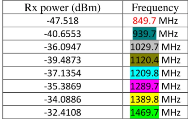
Table (6) lists the peak frequencies and corresponding Rx power. Taking into consideration the non-ideal operating conditions inside the RC, there is an expected difference between the theoretical results and the practical results. It is noted that the peak frequencies are close to the resonance frequencies. At resonance frequencies, the excited modes inside the RC (fmnp) are more effective at resonance frequencies, which make

the Rx power level higher than at non-resonance frequency modes.

Table (7) data was calculated by a Python program to substitute in equation (2.1) by a wide range of m,n,p combinations ( f110, f120, f130, f210,……). Every single parameter m,n,p ranges from 0 to 10, giving a data set of

1000 different values of resonance frequencies from which the data shown in table (6) is extracted, and other frequencies outside the selected bandwidth were excluded. Similar colors in tables (6) and (7) present the frequency at which peak Rx power level occurs and the nearest resonance frequency, respectively.

Table (6) power level (dBm) at peak frequencies Rx power (dBm) Frequency -47.518 849.7 MHz -40.6553 939.7MHz -36.0947 1029.7MHz -39.4873 1120.4MHz -37.1354 1209.8MHz -35.3869 1289.7MHz -34.0886 1389.8MHz -32.4108 1469.7MHz

- 36 -

Table (7) Resonance frequencies of Halmstad University RC at different mode numbers in bandwidth (800MHz-.5GHz) m,n,p resonance frequency 1,3,0 805.7MHz 2,2,1 886.2 MHz 2,3,0 918.7MHz 3,0,1 922.1MHz 3,1,1 956.7MHz 4,0,0 1019.2MHz 0,0,2 1031.6MHz 1,4,0 1050.6MHz 2,3,1 1053.6MHz 0,1,2 1062.6MHz 3,3,0 1081.1MHz 1,1,2 1092.7MHz 2,4,0 1139.5MHz 4,0,1 1142.3MHz 0,2,2 1150.6MHz 1,4,1 1170.4MHz 2,1,2 1178.5MHz 3,3,1 1197.8MHz 4,2,1 1250.8MHz 2,2,2 1258.4MHz 3,4,0 1274.0MHz 0,3,2 1284.0MHz 1,5,0 1299.2MHz 3,1,2 1309.0MHz 5,2,0 1372.2MHz 0,5,1 1374.5MHz 2,3,2 1381.4MHz 5,1,1 1397.9MHz 4,4,0 1441.4MHz 0,4,2 1450.2MHz 2,5,1 1465.9MHz 4,1,2 1472.4MHz 5,3,0 1485.7MHz 3,3,2 1494.3MHz 6,0,0 1528.8MHz

- 37 -

3.3 Quality factor degradation test

The quality factor describes the rate at which a system at resonance loses energy due to its conversion to other forms (e.g. heat)[1]. Mathematically, it is the ratio between the average power inside RC and the dissipated power due to losses. It was measured theoretically and experimentally by a research team from LEMA,

Federal University of Campina Grande, Brazil [21] the experimental results show a higher value of quality factor than the theoretical results do. Two different approaches are considered in another research[20] frequency-domain, and time-domain approaches yield the same measured quality factors. The quality factor of Halmstad University RC has not been measured, so it is not possible to compare it with previous research. Moreover, there is no reference to different losses figures inside the chamber in terms of aperture leakage, conductive and dielectric losses due to the mounting objects inside the chamber. A quality factor degradation test has been conducted by measuring the average Rx power level before and after loading the RC with organic material. The RC was charged by organic material (pieces of wood), which absorb electromagnetic energy and increases the dielectric losses. The quality factor metric reflects the ability of RC to store electromagnetic energy, any conducting or dielectric losses inside RC decrease the stored energy, which means a reduction in quality factor value. Quality factor value measurement is out of the scope of this work. To present an approach of how it affects the stored energy, the average Rx power level was measured before and after loading RC with organic material. The same input power, frequency, and Rx antenna orientation were used before and after RC loading with the organic material. The measurement resulted in a reduction in the average Rx power level by 3.45dB.

- 39 -

4 Conclusion

The field uniformity and isotropy of the electromagnetic wave inside Halmstad University’s reverberation chamber (dimensions are 5.81m,5.81m,2.78m) have been investigated with a tuned-mode mechanical stirrer (rotation step 10 degrees). The focus was on a single-tone continuous sine wave at frequency 2.4GHz. The experimental results show that the field uniformity and isotropy have been verified, and the standard deviation of the measurements (1.464dB) fulfills the IEC 61000-4-21 standards. Sweep measurements of the bandwidth 800MHz-1.5GHz with step 10MHz have been performed. It shows that the Rx power level at the RC resonance frequencies within the sweep bandwidth is remarkably higher than that at other frequencies within the same bandwidth. The quality factor degradation test presents a reduction in the average Rx power by 3.45dBm. While it was outside the scope of this work to measure the quality factor, the test shows clearly that organic material absorbs electromagnetic energy and consequently reduces the stored power in RC. Degradation of the quality factor due to the insertion of organic material has been concluded.

5 Recommendations for continued work

- A unified control system for both the instruments and the stirrer will make the measurement process faster and easier. It will solve the problem of the asynchronous operation of these measurement facilities.

- Installing an extra horizontal stirrer will enhance the stirring effect of the electromagnetic field.

- The control unit of the stirrer needs to be developed to avoid manual reset after every complete execution of the control unit software.

- Interference and unintentional radiations caused by the control unit and its power supply could be avoided by placing them outside the RC, and using fiber cables for connections.

- The lighting system inside the RC uses power cables passing through the RC, which causes EM radiation. If cabling is moved outside the RC its interfering radiation will be eliminated.

- Finally, more accurate and higher resolution measurements can be done by spreading the measuring band width, increasing number of steps of the stirrer during measurement process, and doing the measurements at more points inside the working volume to comply with the IEC 61000-4-21 standards.

RC and environmental tests

Green-house gases carbon dioxide (CO2), water vapor (H2O), methane (CH4), nitrous oxide (N2O) and ozone

(O3) allow the shortwave radiation coming from the sun to pass through the atmosphere. The earth absorbs

sunlight, warms then reradiates heat (infrared or long-wave radiation). The infrared wavelengths that radiated from the earth are supposed to pass through the atmosphere to space, but the green-house gases absorb them. This absorption heats the atmosphere, which in turn re-radiates long-wave radiation in all directions. Some of it makes its way back to the surface of the earth. RC can provide an ideal testing tool to measure different gas density in the air.

The following procedure is a proposed test procedure to use RC in environmental tests, which has not been covered by previous or current RC researches.

- A compressed gas at a specific pressure (gas cylinder) is released inside an RC of a perfect enclosure with no leakage.

- By knowing gas pressure and cylinder volume, its density inside the cylinder can be calculated. - By knowing the RC volume (considering no gas leakage), gas density inside the RC can be obtained.

- 40 -

- RC then is fed by a frequency range which CO2 able to absorb. The received power level at the

receiving antenna indicates how much power is absorbed.

- Repeating the measurements with different gas densities gives a relationship between gas density and power loss due to absorption. This relationship can be used as a reference for testing in other closed or open areas to indicate the gas density.

- Then the same measurement repeated indoors or outdoors (open area) in the environment under test to measure the gas density using the same test antennas which were used.

- The same test can be performed for different types of gases or even water vapor to measure the moisture level. Every gas has a different resonance frequency, which can be determined using the RC.

- 41 -

References

[1] S. J. Boyes and Y. (Electrical engineer) Huang, Reverberation chambers : theory and applications to EMC and antenna measurements. .

[2] J. Carlsson, C. P. Lotback, and A. A. Glazunov, “Reverberation chamber for OTA measurements: The history of a dream!,” 2017 11th Eur. Conf. Antennas Propagation, EUCAP 2017, pp. 237–241, 2017. [3] F. T. Ulaby and U. Ravaioli, Fundamentals of Applied Electromagnetics, ISBN: 978-0-13-335681-6.

2015.

[4] “lines for some of the lower order modes of a rectangular waveguide - ثحب Google.” [Online]. Available:

https://www.google.com/search?q=lines+for+some+of+the+lower+order+modes+of+a+rectangular+ waveguide&safe=active&sxsrf=ALeKk00Fb47crI_eWs6rWFv0OryZarWFyQ:1588120882177&source=ln ms&tbm=isch&sa=X&ved=2ahUKEwjakKuos4zpAhVPwsQBHbcBBWkQ_AUoAXoECAsQAw&biw=1366 &bih=632#imgrc=fLoFuTQrYRItOM. [Accessed: 29-Apr-2020].

[5] K. Selemani, J. B. Gros, E. Richalot, O. Legrand, O. Picon, and F. Mortessagne, “Comparison of reverberation chamber shapes inspired from chaotic cavities,” IEEE Trans. Electromagn. Compat., 2015.

[6] M. H. Nisanci, E. U. Küüksille, Y. Cengiz, A. Orlandi, and A. Duffy, “The prediction of the electric field level in the reverberation chamber depending on position of stirrer,” Expert Syst. Appl., vol. 38, no. 3, pp. 1689–1696, Mar. 2011.

[7] H. Fielitz, K. A. Remley, C. L. Holloway, Q. Zhang, Q. Wu, and D. W. Matolak, “Reverberation-chamber test environment for outdoor urban wireless propagation studies,” IEEE Antennas Wirel. Propag. Lett., vol. 9, pp. 52–56, 2010.

[8] D. B. Nutter, T. W. Leishman, S. D. Sommerfeldt, and J. D. Blotter, “Measurement of sound power and absorption in reverberation chambers using energy density,” J. Acoust. Soc. Am., 2007.

[9] “Radiated immunity tests: reverberation chamber versus anechoic chamber results - IEEE Journals & Magazine.” [Online]. Available: https://ieeexplore-ieee-org.ezproxy.bib.hh.se/document/1658367. [Accessed: 30-Apr-2020].

[10] R. A. Poisel, Antenna systems and electronic warfare applications. .

[11] G. Ultrabroadband, “R & S ® Hl562E Ultralog,” vol. 01, pp. 2017–2018, 2018.

[12] D. G. Fang, Antenna theory and microstrip antennas. CRC Press/Taylor & Francis, 2010. [13] B. Peterson, “Keysight Technologies Spectrum Analysis Basics,” 2013.

[14] A. S. Morris, Measurement and instrumentation principles. Butterworth-Heinemann, 2001. [15] “Search | Rohde & Schwarz.” [Online]. Available:

https://www.rohde-schwarz.com/us/search_63238.html?term=FPC1000. [Accessed: 04-May-2020].