Population and fertility by age and sex for 195 countries and territories, 1950-2017: a systematic analysis for the Global Burden of Disease Study 2017

(1)

This is the published version of a paper published in The Lancet.

Citation for the original published paper (version of record):

Murray, C J., Callender, C., Kulikoff, X R., Srinivasan, V., Abate, D. et al. (2018)

Population and fertility by age and sex for 195 countries and territories, 1950-2017: a

systematic analysis for the Global Burden of Disease Study 2017

The Lancet, 392(10159): 51-2015

https://doi.org/10.1016/S0140-6736(18)32278-5

Access to the published version may require subscription.

N.B. When citing this work, cite the original published paper.

Permanent link to this version:

(2)

Population and fertility by age and sex for 195 countries and

territories, 1950–2017: a systematic analysis for the Global

Burden of Disease Study 2017

GBD 2017 Population and Fertility Collaborators*

Summary

Background

Population estimates underpin demographic and epidemiological research and are used to track progress

on numerous international indicators of health and development. To date, internationally available estimates of

population and fertility, although useful, have not been produced with transparent and replicable methods and do not

use standardised estimates of mortality. We present single-calendar year and single-year of age estimates of fertility

and population by sex with standardised and replicable methods.

Methods

We estimated population in 195 locations by single year of age and single calendar year from 1950 to 2017

with standardised and replicable methods. We based the estimates on the demographic balancing equation, with

inputs of fertility, mortality, population, and migration data. Fertility data came from 7817 location-years of vital

registration data, 429 surveys reporting complete birth histories, and 977 surveys and censuses reporting summary

birth histories. We estimated age-specific fertility rates (ASFRs; the annual number of livebirths to women of a

specified age group per 1000 women in that age group) by use of spatiotemporal Gaussian process regression and used

the ASFRs to estimate total fertility rates (TFRs; the average number of children a woman would bear if she survived

through the end of the reproductive age span [age 10–54 years] and experienced at each age a particular set of ASFRs

observed in the year of interest). Because of sparse data, fertility at ages 10–14 years and 50–54 years was estimated

from data on fertility in women aged 15–19 years and 45–49 years, through use of linear regression. Age-specific

mortality data came from the Global Burden of Diseases, Injuries, and Risk Factors Study (GBD) 2017 estimates. Data

on population came from 1257 censuses and 761 population registry location-years and were adjusted for

underenumeration and age misreporting with standard demographic methods. Migration was estimated with the

GBD Bayesian demographic balancing model, after incorporating information about refugee migration into the model

prior. Final population estimates used the cohort-component method of population projection, with inputs of fertility,

mortality, and migration data. Population uncertainty was estimated by use of out-of-sample predictive validity testing.

With these data, we estimated the trends in population by age and sex and in fertility by age between 1950 and 2017 in

195 countries and territories.

Findings

From 1950 to 2017, TFRs decreased by 49·4% (95% uncertainty interval [UI] 46·4–52·0). The TFR decreased

from 4·7 livebirths (4·5–4·9) to 2·4 livebirths (2·2–2·5), and the ASFR of mothers aged 10–19 years decreased from

37 livebirths (34–40) to 22 livebirths (19–24) per 1000 women. Despite reductions in the TFR, the global population

has been increasing by an average of 83·8 million people per year since 1985. The global population increased by

197·2% (193·3–200·8) since 1950, from 2·6 billion (2·5–2·6) to 7·6 billion (7·4–7·9) people in 2017; much of this

increase was in the proportion of the global population in south Asia and sub-Saharan Africa. The global annual rate

of population growth increased between 1950 and 1964, when it peaked at 2·0%; this rate then remained nearly

constant until 1970 and then decreased to 1·1% in 2017. Population growth rates in the southeast Asia, east Asia, and

Oceania GBD super-region decreased from 2·5% in 1963 to 0·7% in 2017, whereas in sub-Saharan Africa, population

growth rates were almost at the highest reported levels ever in 2017, when they were at 2·7%. The global average age

increased from 26·6 years in 1950 to 32·1 years in 2017, and the proportion of the population that is of working age

(age 15–64 years) increased from 59·9% to 65·3%. At the national level, the TFR decreased in all countries and

territories between 1950 and 2017; in 2017, TFRs ranged from a low of 1·0 livebirths (95% UI 0·9–1·2) in Cyprus to a

high of 7·1 livebirths (6·8–7·4) in Niger. The TFR under age 25 years (TFU25; number of livebirths expected by age

25 years for a hypothetical woman who survived the age group and was exposed to current ASFRs) in 2017 ranged

from 0·08 livebirths (0·07–0·09) in South Korea to 2·4 livebirths (2·2–2·6) in Niger, and the TFR over age 30 years

(TFO30; number of livebirths expected for a hypothetical woman ageing from 30 to 54 years who survived the age

group and was exposed to current ASFRs) ranged from a low of 0·3 livebirths (0·3–0·4) in Puerto Rico to a high of

3·1 livebirths (3·0–3·2) in Niger. TFO30 was higher than TFU25 in 145 countries and territories in 2017. 33 countries

had a negative population growth rate from 2010 to 2017, most of which were located in central, eastern, and western

Europe, whereas population growth rates of more than 2·0% were seen in 33 of 46 countries in sub-Saharan Africa.

In 2017, less than 65% of the national population was of working age in 12 of 34 high-income countries, and less than

50% of the national population was of working age in Mali, Chad, and Niger.

Lancet 2018; 392: 1995–2051

*Collaborators listed at the end of the paper

Correspondence to: Prof Christopher J L Murray, Institute for Health Metrics and Evaluation, Seattle, WA 98121, USA

(3)

Introduction

Age-sex-specific estimates of population are a bedrock of

epidemiological and economic analyses, and they are

integral to planning across several sectors of society. As

the denominator for most indicators, such estimates

permeate every aspect of our understanding of health

and development. Errors in population estimates affect

national and international target tracking and time-series

and cross-country analyses of development outcomes.

The impor tance of accurate population estimates for

government planning cannot be overstated: population

size, age, and composition dictate the national need for

infrastructure, housing, education, employment, health

care, care of older people, electoral representation,

provision of public health and services, food supply, and

security.

1

_{Similarly, fertility rates, both by maternal age}

and overall, are key drivers of population growth and

important social outcomes in their own right.

Many governments typically produce national

popu-lation estimates by age and sex for planning purposes.

Most international studies and comparative indicators,

including the Millennium Development Goals and the

Sustainable Development Goals, rely on the estimates

generated by the UN Population Division at the

Department of Economics and Social Affairs (UNPOP)

for population denomi nators,

2,3

_{although it is not well}

documented how often these estimates are used by

national governments. The UNPOP has produced

population estimates since 1951, and it uses a

de-centralised approach to estimation.

4

_{For example, the}

Latin American and Caribbean Demographic Centre

produces estimates for Latin America, whereas estimates

for all other groups of countries

are developed by analysts

in New York. Although the UNPOP describes a general

approach of examining data on fertility, mortality,

migration, and population and searching for consistency,

5

replicable statistical methods are not used. Decisions on

how to deal with inconsistency between the

compo-nents of fertility, mortality, and migration within

population counts are left to individual analysts, leading

to considerable hetero

geneity in approaches across

countries. Accordingly, discrepancies between UNPOP

and nationally produced estimates—for instance, in

2015, the population estimates for Mexico by UNPOP

were 4·6 million more than those of Mexico’s National

Population Council (125·9 million by UNPOP vs

Interpretation

Population trends create demographic dividends and headwinds (ie, economic benefits and detriments)

that affect national economies and determine national planning needs. Although TFRs are decreasing, the global

population continues to grow as mortality declines, with diverse patterns at the national level and across age groups.

To our knowledge, this is the first study to provide transparent and replicable estimates of population and fertility,

which can be used to inform decision making and to monitor progress.

Funding

Bill & Melinda Gates Foundation.

Copyright

© 2018 The Author(s). Published by Elsevier Ltd. This is an Open Access article under the CC BY

4.0 license.

Research in context

Evidence before this study

Population estimates by age and sex are extensively used in all

forms of epidemiological and demographic analysis. National

estimates of population and fertility for age and sex groups

have been produced by the UN Population Division since 1951.

The US Census Bureau produces revised demographic estimates

for 15 to 30 countries each year. Several national authorities

produce their own population estimates, particularly those in

high and middle Socio-demographic Index countries. These

efforts are all based on the cohort-component method of

population projection, namely that population in an age group

at a given time t must equal the population in that cohort at

the start of the time period (t–1) plus new entrants and minus

people exiting the population because of migration and death.

Although these estimates are based on the demographic

balancing equation, estimates are not based on standardised,

transparent, or replicable statistical methods.

Added value of this study

To our knowledge, this study presents the first estimates of

population by location from 1950 to 2017 that are based on

transparent data and replicable analytical code, applying a

standardised approach to the estimation of population for each

single year of age for each calendar year from 1950 to 2017 for

195 countries and territories and for the globe. This study

provides improved population estimates that are internally

consistent with the Global Burden of Diseases, Injuries, and Risk

Factors Study’s assessment of fertility and mortality, which are

important inputs to other epidemiological research and

government planning.

Implications of all the available evidence

Population counts by age and sex that are produced with a

transparent and empirical approach will be useful for

epidemiological and demographic analyses. The production of

annual estimates will also facilitate timely tracking of progress

on global indicators, including the Sustainable Development

Goals. In the future, the methods applied here can be used to

enhance population estimation at the subnational level.

(4)

121·3 million by National Population Council)—cannot

currently be resolved.

4,6

The US Census Bureau’s International Division

periodically releases detailed population analyses for

selected countries, with new revisions produced for

15 to 30 countries per year.

7

_{Other organisations, such as}

the Population Reference Bureau,

8

_{the World Bank,}

9

the Wittgenstein Centre,

10

_{and Gapminder Foundation}

11

also release population estimates, but these are largely

combinations of national estimates with selected UNPOP

or US Census Bureau analyses. Many of the

organi-sations who estimate or report on population also

provide fertility estimates, which, in addition to affecting

population trends, are used to monitor reproductive

health service delivery in many locations. To our

knowledge, global estimates of annual population by age

and sex with underlying primary data and replicable

computer code and statistical modelling details are not

available from any source.

The Global Burden of Diseases, Injuries, and Risk

Factors Study (GBD) is committed to the Guidelines on

Accurate and Transparent Health Estimates Reporting

(GATHER).

12

_{Continued use of the UNPOP population}

estimates in GBD is not compatible with GATHER

because the methods used for UNPOP estimation are

not transparent and uncertainty intervals are not

estimated for populations.

4

_{Moreover, UNPOP population}

esti mates, especially in years between or after a census,

are inconsistent with GBD estimates because there is a

marked difference between UNPOP and GBD estimates

of age-specific mortality in many instances.

13,14

_{For this}

GBD 2017 paper, we sought to produce population

estimates and associated fertility estimates for

195 countries and territories from 1950 to 2017 that were

based on the available census or population registry data

and survey and census data on age-specific fertility rates

(ASFR; ie, the annual number of livebirths to women of a

specified age group per 1000 women in that age group)

by use of replicable methods, leveraging the previous

GBD work that estimated age-sex-specific mortality

rates.

15

_{To achieve this goal, we aimed to conduct}

systematic analyses of available sources that could

inform ASFR estimation and to systematically identify

and extract census and population registry data.

Methods

Overview

As with all population estimation, the underlying

equation used for GBD is based on the demographic

balancing equation

16

where N (T) is the population at a given time, N (0) is the

population at the start of the interval, B (0,T) is livebirths

during

the interval, D (0,T) is deaths during

the interval,

and G (0,T) is net migration during the interval.

The cohort-component method of population pro jection

extends this demographic balancing equation to estimate

internally consistent age-sex-specific popu

lations. The

method requires estimates of ASFRs, sex ratio at birth,

age-sex-specific net migration, and age-sex-specific

mor-tality rates that are

consistent with observed population

counts that have been corrected for underenumeration or

overenumeration. GBD provides a consistent set of

age-sex-specific mortality rates with standardised methods;

15

_in

this analysis, we estimated the sex ratio at birth, ASFR, and

age-sex-specific migration rates consistent with the

available population data to create a full time series of

population

estimates by age and sex.

These estimates comply with GATHER (appendix 1

section 5). Analyses were done with R version 3.3.2, Python

version 2.7.14, or Stata version 13.1. Data and statistical

code for all analyses are publicly available online.

Geographical units and time periods

We produced single calendar-year and single

year-of-age population estimates

for 195 countries and territories

that were grouped into 21 regions and seven

super-regions. The seven super-regions are central Europe,

eastern Europe, and central Asia; high income;

Latin America and the Caribbean; north Africa and the

Middle East; south Asia; southeast Asia, east Asia, and

Oceania; and sub-Saharan Africa. Each year, GBD includes

sub

national analyses for a few new countries and

continues to provide subnational estimates for countries

that were added in previous cycles. Subnational estimation

in GBD 2017 includes five new countries (Ethiopia, Iran,

New Zealand, Norway, Russia) and countries previously

estimated at subnational levels (GBD 2013: China, Mexico,

and the UK [regional level]; GBD 2015: Brazil, India,

Japan, Kenya, South Africa, Sweden, and the USA; GBD

2016: Indonesia and the UK [local government authority

level]). All analyses are at the first level of administrative

organisation within each country except for New Zealand

(by Māori ethnicity), Sweden (by Stockholm and

non-Stockholm), and the UK (by local government authorities).

All subnational estimates for these countries were

incorporated into model development and evaluation as

part of GBD 2017. To meet data use requirements, in this

publication we present all subnational estimates excluding

those pending publication (Brazil, India, Japan, Kenya,

Mexico, Sweden, the UK, and the USA); given space

constraints, these results are presented in appendix 2

instead of the main text. Subnational estimates for

countries with populations of more than 200 million

people (assessed by use of our most recent year of

published estimates) that have not yet been published

elsewhere are presented wherever estimates are

illus-trated with maps but are not included in tables. Estimates

were produced for the years 1950–2017. 1950 was selected

as the start year for the analysis because we were unable to

locate sufficient data on ASFR, mortality, and population

before 1950.

N(T)=N(0) + B(0,T) – D(0,T) + G(0,T)

See Online for appendix 1

For the statistical code see http://ghdx.healthdata.org/gbd-2017

(5)

Fertility

Fertility data are obtained from vital registration systems,

complete birth histories, or summary birth histories.

Complete birth histories include the date of birth and, if

applicable, the dates of death of all children ever born

alive to each woman that is interviewed, whereas

summary birth histories include the total number of

children ever born alive to each mother and the total

number of those children born alive to each mother that

have died. In countries with complete birth registration,

vital registration

systems typically provide tabulations of

births by age of the mother. From 1890,

17

_{some censuses}

asked about the number of children ever born to a

woman, and this question has been widely asked in

censuses and many household surveys in the past

70 years. From the 1970s, fertility information has also

been collected through complete birth histories,

beginning with the World Fertility Survey, then the

Demographic and Health Surveys, and, in some

countries, the Multiple Indicator Cluster Surveys,

977 censuses and household surveys that had summary

birth history data, 429 household surveys that had

complete birth history data, and 7817 country-years of

birth registration systems through searches of national

statistical sources and the Demographic Yearbooks

produced by the UN Statistics Division from 1948 to

present.

18

_{The number and type of sources for each}

location are provided in appendix 1 (section 5). The

Global Health Data Exchange provides the metadata for

all these sources.

Given the hetergeneous

nature of the data (vital

registration, summary birth histories, complete birth

histories), we used a two-stage approach to modelling the

ASFR for the age groups 15–19 years, 20–24 years,

25–29 years, 30–34 years, 35–39 years, 40–44 years, and

45–49 years. The two-stage approach was designed to take

advantage of the greater availability of some summary

birth history data for the period 1950 to 1975 and to help

to compensate for

the lower availability of complete birth

history data in some low-income countries. For the

fertility rates in those aged 10–14 years and 50–54 years,

which are much lower than in other age groups and for

which only vital registration data were available, we used

a separate, simpler approach, described later in this

section.

In the first stage of our analysis, we used spatio temporal

Gaussian process regression to analyse vital registration

and complete birth history data.

15,19

_{For spatiotemporal}

Gaussian process regression, the prior was estimated

separately for women aged 20–24 years, with average years

of schooling in women aged 20–24 years as the covariate.

For all other age groups, the prior was estimated with a

spline on the estimated ASFR for women aged 20–24 years

and with the average years of schooling for the age group

of interest. The prior for GBD locations in the

high-income super-region did not include average years of

schooling as a covariate. Spline knots were selected by

inspection of the data to identify where there was a

reversal in trend. The purpose of this approach was to

capture an increase in fertility rates in women aged

30 years or older while the ASFR for women aged

20–24 years decreased below a specific threshold. Given

that the point of inflection for the ASFR for women aged

30 years or older relative to the ASFR for women

aged 20–24 years varied by super-region, we fit the models

separately for some GBD super-regions (high income;

sub-Saharan Africa; and central Europe, eastern Europe,

and central Asia) and modelled the rest of the

super-regions together. The first step of the model also included

location-and-source-specific random effects to correct bias

from non-sampling error in different source types, such

as incomplete vital registration. Hyperparameters for the

model were selected on the basis of a measure of data

density. Further details on this process are provided in

appendix 1 (section 2).

In the second stage of the analysis, we used the

ASFR estimates from the first stage to process and

incorporate several forms of aggregated data. First, we

split cumulative cohort fertility data (ie, children ever

born) from summary birth history into period ASFR data.

For this split, we computed the ratio between reported

children ever born alive from each 5-year cohort of women

represented in a given data source and the total fertility for

each of these cohorts that was implied by the first-stage

estimates of ASFR by location and year. This ratio

was applied as a scaling factor to our estimated cohort

ASFR at 5-year intervals (when all members of the cohort

all belong to a single 5-year GBD age group), to distribute

experienced fertility (ie, from age 10 years until the date of

the survey in women interviewed from the cohorts

specified in the original data) back across age and time.

Additionally, we used the estimated age proportion of

livebirths from the first stage to distribute total reported

livebirths by the age of the mother. Lastly, for historical

location aggregates for which we had registry data (eg, the

Soviet Union), we used the estimated proportions of

age-specific livebirths in constituent locations from the first

stage to allocate births back in time to their current

GBD geographies. This new set of methods allowed us to

supplement the model with a substantial amount of

additional information about the overall fertility. We then

re-estimated ASFR as described, with all vital registration,

complete birth history, and split data to produce final

fertility estimates for women aged 15–49 years.

In both the first and second stage, data were adjusted in

the mixed-effects model on the basis of random

effects values (appendix 1 section 2)

by selecting a

reference or benchmark source. In locations with

complete child death registration (see previous GBD

analyses),

15,20

_{vital registration was typically the benchmark}

or reference source. In other locations, Demographic and

Health Survey complete birth history data were used as

the reference source. If neither vital registration nor

For the Global Health Data

Exchange see http://ghdx.

(6)

Demographic and Health Survey complete birth histories

were available, other complete birth history sources were

used as the reference. If no vital registration or complete

birth history data were used, then the average of all

remaining summary birth history sources were used as

reference. Where sources were inconsistent or

implausible time trends were identified, some reference

source designations were modified; the final choice of

reference sources for each location are provided in the

appendix 1 (section 5).

Many household surveys on fertility excluded women in

the age groups 10–14 years and 50–54 years, and

these data were limited to 3947 country-years of vital

registration data. To estimate fertility in girls aged

10–14 years, we used a linear regression of the log of the

ratio of the ASFR of girls aged 10–14 years to the ASFR for

girls aged 15–19 years as a function of the ASFR for girls

aged 15–19 years. For women aged 50–54 years, we found

no covariates that predicted variation in the ratio of ASFR

for women aged 50–54 years to the ASFR for those aged

45–49 years. In this case, we assumed the ratio of ASFR

for women aged 50–54 years to ASFR for women aged

45–49 years was constant across locations and over time.

Our analysis generated a full set of ASFRs for each

location and year from 1950 to 2017; we used these ASFRs

to compute the total fertility rate (TFR), which is the

average number of children a woman would bear if she

survived through the end of the reproductive age span

(age 10–54 years) and experienced at each age a particular

set of ASFRs observed in the year of interest. We also

estimated the total fertility rate under age 25 years

(TFU25; number of livebirths expected by age 25 years for

a hypothetical woman who survived the age group and

was exposed to current ASFRs) and the total fertility in

women older than 30 years (TFO30; number of livebirths

expected for a hypothetical woman ageing from 30 to

54 years who survived the age group and was exposed to

current ASFRs). These age ranges were computed

because nearly all locations show decreases in the TFU25

over time, with few or no reversals. In women aged 30

years or older, there is a clear U-shaped curve, with

decreases followed by sustained increases; in women

aged 25–29 years, the pattern is less consistent. The

fertility rate in girls aged 10–19 years is a Sustainable

Development Goal (SDG) indicator for goal 3, target 3.7:

ensure universal access to sexual and reproductive

health-care services, including for family planning, information

and education, and the integration of reproductive health

into national strategies and programmes.

21

We estimated the sex ratio at birth with 4690 unique

years of registered livebirths by sex, 1756

location-years of census and population registry counts that

included children younger than 1 year and younger than

5 years by sex, and 2490 location-years of the proportion

of live-born males from complete birth history. These

data informed a spatiotemporal Gaussian process

regression model of the proportion of live-born males,

assuming a time-invariant prior for the mean because, in

the absence of sex-selective abortion, we would not expect

the sex ratio at birth to deviate significantly from its

natural equili brium. Hyperparameters for spatiotemporal

smoothing and Gaussian process regression were chosen

on the basis of data-density scores, taking into account

both the quantity and quality of available data. Our

analysis only produced national estimates of sex ratio at

birth—including for Hong Kong and Macau—for all

years from 1950 to 2017; thus, we assume that subnational

sex ratio at birth equals the national sex ratio at birth.

With additional data seeking and extraction, we will

extend the analysis to all GBD locations in the next GBD

study. Further details regarding sex ratio at birth

estimation are shown in appendix 1 (section 2).

Population

To determine national and subnational populations, we

searched the Integrated Public Use Microdata Series

questionnaires, the UN Demographic Yearbook, the UN

census programme census dates, and the International

Population Census Biography to identify all censuses

conducted between 1950 and 2017 and available

popu-lation registers.

22–25

_{We included 1233 censuses and}

26 population registers that contained 730 location-years

of census or population registry data. In some cases,

the same census was reported by different sources

in different years. We resolved these incon sistencies

through a review of available documentation. A list of

all confirmed censuses is shown in the appendix 1

(section 5). We obtained population counts that were

age-sex-specific from 1171 censuses and only by sex from

62 censuses. We sought to identify whether the counts in

each census were de facto (allocated to the place of

enumeration) or de jure (allocated to the place of regular

or legal residence). Our basis for population estimation

is the de-facto population and, where both counts were

available, we used de-facto counts. Where only de-jure

counts were available—typically in lower

Socio-demographic Index (SDI) countries—we assumed that

de-jure and de-facto populations were similar. The main

difference between the counts at the national level is the

exclusion of some migrant workers in some de-jure

counts; where migrant workers are known to be an

important fraction of the population and de-facto counts

were not available, we searched directly for data on

documented migration.

In several cases, the UN does not recognise

admin-istrative splits in territories, including Kosovo and

Serbia, Transnistria and Moldova, and the so-called

Turkish Republic of Northern Cyprus and Cyprus.

26

In these cases, we obtained census counts for the

components and interpolated to generate census counts

for the full territory. For east and west Germany before

unification, as the input to the model, we used census

counts for each component and interpolation to

generate estimates of joint census counts in years

(7)

closest to the censuses in both locations. We were able

to obtain census counts for five of the six constituent

components that made up Yugoslavia; for Serbia we

split aggregate Yugoslavia census data with previous

population estimates. For Singapore, we estimated the

population for residents and non-resident workers

combined (appendix 1 section 2). Of the 1963

location-years of census or population registry data,

72 lo cation-years were identified as outliers that were

inconsistent with adjacent data, model analysis, or

excluded subpopulations.

Census counts are typically undercounts of the actual

population, although there are known cases in which

censuses have overcounted the population.

27–29

Post-enumeration surveys (PESs) aim to identify instances of

overcounts or undercounts by comparing data. Many, if

not most, PESs are not published or are only reported in

government releases, presentations, or online reports.

PESs themselves are subject to considerable error, whether

they use a direct or indirect method of estimating census

completeness. We searched for all available PES results

and supple

mented these results with publications or

presentations that provided summaries of other PESs.

30–34

We identified 165 PESs, although it is likely that many

more were done that did not publicly report their results.

We analysed the 165 PESs to generate a general model of

census com pleteness as a function of SDI. Because of

variable quality of PESs, we assumed that, in aggregate,

the 165 PESs provided an unbiased view of the association

between enumeration completeness and SDI, so we

adjusted census counts by the predictions from this model.

We used nationally reported PES results to adjust census

counts in high SDI countries and used the estimated

census completeness to adjust data in other settings.

To account for systematic age variation in census

enumeration, we input age-sex-specific PES results into

DisMod-MR 2.1, a Bayesian meta-regression tool, to

estimate a global age pattern of enumeration. This age

pattern was then used to adjust the overall predicted

enumeration to vary by age (appendix 1 section 2).

As has been extensively noted in the demographic

literature, census counts have several common problems:

undercounts (particularly of children younger than

5 years), a tendency to exaggerate age at older ages, and

age heaping (reporting ages rounded to the nearest

5 or 10 years).

35–38

_{The population counts from}

four different censuses, illustrating the different types of

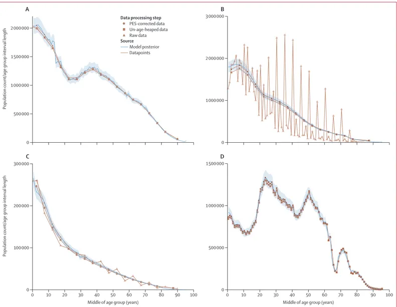
age heaping and undercounts, are shown in figure 1. We

evaluated the age structure and consistency of census

data by calculating sex and age ratios for each census.

These ratios were then used to calculate sex and age ratio

scores, which were combined into a joint score. The joint

score was used to determine whether to apply a correction

to the census counts or not. For census counts available

in 1-year age groups, we used the Feeney correction;

for counts available in

5-year or 10-year age groups, we

used either the Arriaga or Arriaga strong correction.

39,40

More details on the age-heaping corrections are shown in

appendix 1 (section 2). For all censuses in low and middle

SDI countries, we did not use the census count of

children younger than 5 years in our model estimation.

In other words, population estimates in these age groups

were driven by fertility and mortality estimates and

consistency with the later census counts for the same

cohort. Systematic over estimation of age, particularly in

some countries in sub-Saharan Africa and Latin America,

was apparent in the data; for example, census counts

could only be explained by large immigration of

populations at older ages, which appears implausible.

We were unable to correct the data for these issues and

used the modelling strategy that is subsequently

described to deal with these challenges.

Our approach requires an estimate of the population

in 1950 in all locations for detailed age and sex groups;

only 54 countries had a census count in 1950. For

most other locations, we used backwards application of

the cohort-component method of population projection by

use of the oldest available census and the reverse

application of estimated mortality rates and an assumption

of zero net migration (appendix 1 section 2). As

sub-sequently noted, in our GBD Bayesian demographic

balancing modelling framework, the base line population

is assumed to be measured with substantial error, and

the model produced posterior estimates that varied

considerably from this initial baseline.

We used the estimates of population by location and

year for each single year of age to generate other

summary measures, including population growth rates

that assumed logarithmic growth and the proportion

of the population that was of working age, which is

defined by the Organisation for Economic Co-operation

and Development and the World Bank as those aged

15–64 years.

41,42

Mortality

The GBD mortality process produced annual abridged life

tables that comprised 24 age groups: younger than 1 year,

1–4 years, and then 5-year age groups up to age 110 years

or older.

13

_{To project populations forwards in time with the}

cohort-component method of population projection, we

needed annual period life tables with single-year age

groups up to 95 years or older. For ages 15–99 years, we

interpolated abridged l

x

values (the number of people still

alive at age x for a hypothetical cohort in a period life table)

by use of a monotone cubic spline with Hyman filtering.

43,44

For people younger than 15 years and older than 100 years,

we applied regression coeffi cients to predict single-year

age group probability of death values. The Human

Mortality Database provided 4557 empirical full-period life

tables for 48 locations. We excluded 1280 of the life tables

because they were identified by the Human Mortality

Database as proble matic or occurred during time periods

with extremely high mortality, such as World War 2 or

the 1918 influenza pandemic. To predict probability of

(8)

death q

x

at age x for single-year age groups, we fit the

following separate linear regression by single-year age

group between ages zero and 110:

where

1

q

xf

is the single-year age group q

x

value from the

full-period

life table, β

0

is the coefficient for the intercept, β

1

is

the coefficient for the slope, ε

xf

is the error term, and

5

q

xa

is

the correponding abridged life-table age group’s q

x

value.

These predicted

1

q

xf

values were scaled to the GBD abridged

life-table

5

q

x

values for consis tency.

For those aged 15–99 years, the non-parametric spline

approach did not require rescaling to match the abridged

5

q

x

values and, consequently, produced smooth steps

in mortality across single-year ages and between 5-year

age groups. The regression coefficients were applied to

children younger than 15 years because of the unique

patterns of single-year mortality younger than 15 years

and to adults older than 100 years because of instability

caused by low l

x

values at older ages. To mitigate instability

caused by spikes in mortality due to fatal discontinuities

such as wars and natural disasters, full-period life tables

were first generated based on abridged life tables without

fatal discontinuities, and then fatal discontinuities were

added to

n

m

x

(the death rate in age group x to x + 1 for a

hypothetical cohort in a period life table) assuming a

constant death rate for fatal discontinuities within each

age group. To produce full life tables with the complete

set of single-year age group

1

q

x

values, we assumed

1

a

x

(the

average number of years lived in age group x to x + 1 by

people who died during the interval for a hypothetical

log(

1

q

x_f

)=β

0

+ β

1

log(

5

q

xa

) + ε

xf Model posterior Datapoints Source PES-corrected data Un-age-heaped data Raw data

Data processing step

0 500 000 1 000 000 1 500 000 2 000 000

Population count/age group interval length

A

0 1 000 000 2 000 000 3 000 000

B

0 10 20 30 40 50 60 70 80 90 100 0 100 000 200 000 300 000

Population count/age group interval length

Middle of age group (years)

C

0 10 20 30 40 50 60 70 80 90 100 0 500 000 1 000 000 1 500 000

Middle of age group (years)

D

Figure 1: Census age patterns for females in 1970 in the USA (A), males in 2001 in Bangladesh (B), females in 1979 in Afghanistan (C), and males in 2010 in Russia (D)

Lines show the model posterior and datapoints. Data processing steps are indicated by symbols. The 95% uncertainty interval is shown by light blue shading around the model posterior. PES=post-enumeration survey.

(9)

cohort in a period life table) was 0·5 in all age groups

except for those younger than 1 year and older than

110 years; these groups were assumed to be identical to

the abridged life-table

1

a

x

values.

Migration

Real data on age-specific net migration are more difficult

to obtain than data on fertility, population, and mortality.

Net migration includes any change in the de-facto

population that is not accounted for by births or deaths;

this number would include refugees and temporary

workers. For most country-years, documented net

migration data are not reported and undocumented net

migration is not estimated. For some high-SDI countries,

net migration is tracked and reported,

45

_{and the UN High}

Commission for Refugees (UNHCR) reports the stock of

refugees (the count of people not born in the country that

they currently live in) in each country by country of origin

at the end of year. In more recent census rounds, census

questions on the number of foreign-born individuals

living in a country have been used, as have assumptions

on differential survival to estimate when migration

occurred;

46

_{however, these approaches, especially for the}

period before 2000, have considerable uncertainty

associated with them and are heavily dependent on

fertility and mortality assum ptions for migrants.

We developed and applied the GBD Bayesian

demo-graphic balancing model to estimate net migration by

single year of age and single calendar year, consistent

with our estimates of age-sex-specific mortality and

ASFR and the observed population data. Our model was

developed on the basis of the work of Wheldon and

colleagues

47–49

_{but includes important modifications, such}

as correlation of migration rates across ages and over

time and single-year, single-age estimation. Details on

our GBD Bayesian demographic balancing model,

developed in Template Model Builder, an open-source

statistical package for R,

50

_{are shown in the appendix 1}

(section 2).

In applying the model, we dealt with known issues of

age misreporting by including larger input data variance

for population counts at the youngest ages and input

variance that steadily increases after age 45 years. The

choice of data variance was based on testing of a range of

variance assumptions; variance assumptions only change

the point estimates of the results in settings where there

is substantial inconsistency between adjacent census

counts or between census counts (or both) and in the

key inputs. To address age misreporting in the oldest

ages, we ran several model versions for each location. For

each model version, we excluded census counts above a

given maximum age from the model fitting process

(appendix 1 section 5). We then selected the best model

version by prioritising versions that used the highest

maximum age, predicted low absolute values of migration

in the age groups older than 55 years, and had good

in-sample fits. In high-income locations, the selection

algorithm often chose the model version that did not

exclude any of the census data for older ages but, in other

regions, the population estimates at older ages were

driven by the census counts for younger ages and the

mortality estimates that aged those people forwards in

time

(appendix 1 section 2).

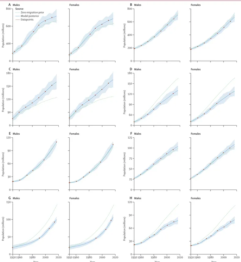
An example of the fit to the available population data for

the eight largest populations in 2017 is shown in figure 2.

Overall, the in-sample fit of the model for age-sex-specific

population log space had an R² value of 0·99. These fits

show that the model closely tracks the available corrected

census counts for all ages combined and by age. Code

for the GBD Bayesian demographic balancing model

is available at the Global Health Data Exchange. The

population estimates and census and registry data for all

195 countries and territories are shown in appendix 2.

The cohort-component method of population

projection and uncertainty

We produced final population estimates by single year and

by single-year age groups with the cohort-component

method of population projection.

16

_{The population}

_in

each single-year age group in each year was estimated

on the basis of the estimated starting population and

single-year, single-age rates of migration, fertility, and

mortality. Uncertainty in population estimates comes

from two fundamental sources: uncertainty about the

complete ness of a census count in a census year and

uncertainty between censuses due to errors in estimates

of migration, fertility, and mortality. Uncertainty in the

counts was estimated by sampling the variance-covariance

matrix of the model that predicted census completeness.

We estimated the uncertainty between counts by use

of out-of-sample predictive validity. We held out data

and estimated the error in estimates as a function of

the minimum of the number of years to the next

or previous census. We combined these two sources of

uncertainty and generated 1000 draws of percentage error

in the population for each location-year. The 1000 draws of

percentage error in the population and the population

mean, generated by the GBD Bayesian demographic

balancing model, were then combined to create 1000 draws

of population by age, sex, location, and year. 95%

uncer-tainty intervals (UIs) were calculated with the 2·5th and

97·5th percentiles. Details of this out-of-sample estimation

of uncertainty are shown in appendix 1 (section 2).

Out-of-sample estimates of uncertainty yielded larger uncertainty

than in-sample methods because of the nearly perfect

inverse correlation between migration and death rates,

which was conditional on census counts with low error.

A dot plot comparison of our total population counts by

country for different age groups in 2017 with UNPOP

estimates is shown in appendix 2.

SDI

GBD 2015 developed the SDI as a composite measure of

TFR in a population, lag-distributed income per capita,

(10)

1950 1960 1980 2000 2020 0 50 100 150 Population (millions) Year

G

Males 1950 1960 1980 2000 2020 Year Females 1950 1960 1980 2000 2020 0 30 90 120 Population (millions) Year

H

Males 1950 1960 1980 2000 2020 60 Year Females 0 60 90 120 Population (millions)

E

Males 30 Females 0 25 100 125 Population (millions)

F

Males 75 50 Females 0 90 150 180 Population (millions)

C

Males 120 Females 0 90 120 180 Population (millions)

D

Males 60 150 Females 0 400 600 800 Population (millions)

A

Males Females 0 400 600 800 Population (millions)

B

Males 200 Females

Zero migration prior Model posterior Datapoints

Source

Figure 2: Fit of the GBD Bayesian demographic balancing model for the total population of males and females, from 1950 to 2017, in mainland China (A), India (B), the USA (C), Indonesia (D),

Pakistan (E), Brazil (F), Nigeria (G), and Bangladesh (H)

The 95% uncertainty interval is shown by light blue shading around the model posterior line. Mainland China excludes Hong Kong and Macao. GBD=Global Burden of Diseases, Injuries, and Risk Factors Study.

(11)

and average years of education in the population older

than 15 years.

15,20

_{Each component was rescaled to a value}

between 0 and 1, and the SDI was derived from their

geometric mean. The TFR was used in this overall

measure of development as a proxy for the status of

women in society; other plausible measures capturing

the status of women are not available for all countries

over a long time period. Our analysis of detailed ASFR

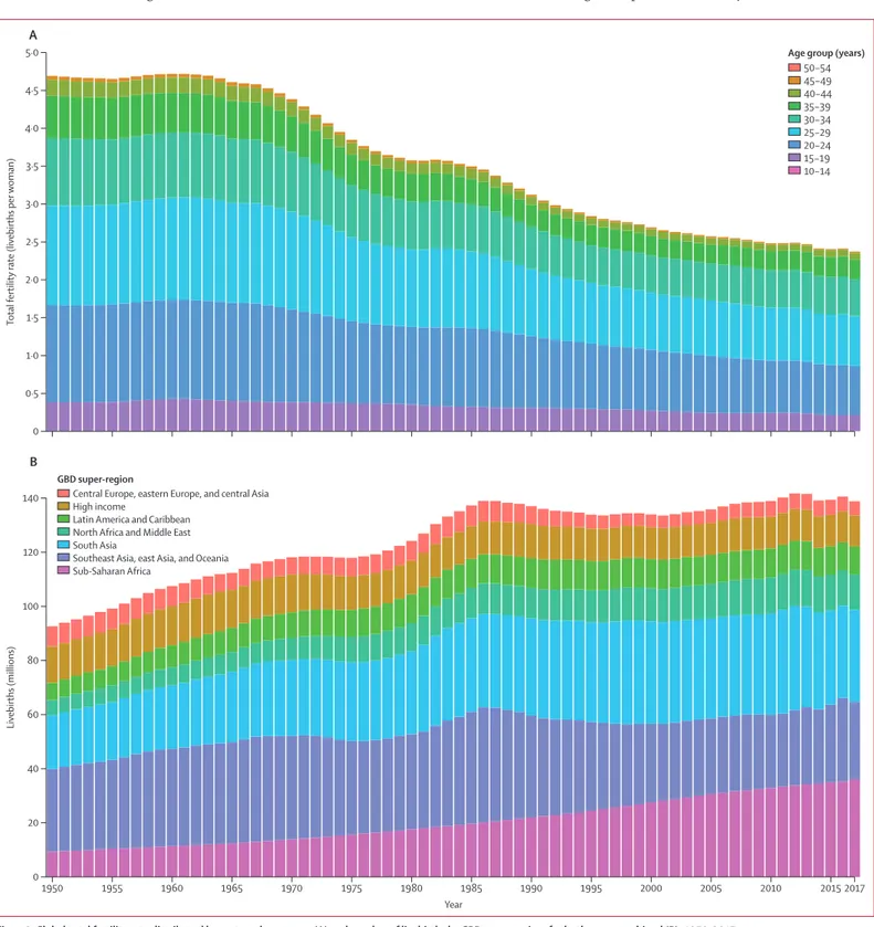
0 0·5 1·0 1·5 2·0 2·5 3·0 3·5 4·0 4·5 5·0

Total fertility rate (livebirths per

woman)

A

1950 1955 1960 1965 1970 1975 1980 1985 1990 1995 2000 2005 2010 2015 2017 0 20 40 60 80 100 120 140 Livebirths (millions) Year

B

Age group (years)

50−54 45−49 40−44 35−39 30−34 25−29 20−24 15−19 10−14 GBD super-region

Central Europe, eastern Europe, and central Asia High income

Latin America and Caribbean North Africa and Middle East South Asia

Southeast Asia, east Asia, and Oceania Sub-Saharan Africa

Figure 3: Global total fertility rate distributed by maternal age group (A) and number of livebirths by GBD super-region, for both sexes combined (B), 1950–2017

Total fertility rate is the number of births expected per woman in each age group if she were to survive through the reproductive years (10–54 years) under the age-specific fertility rates at that timepoint. GBD=Global Burden of Diseases, Injuries, and Risk Factors Study.

(12)

revealed in many countries that, through the process of

development the TFO30 generally decreased and then

increased. For example, in the USA, the TFO30 has

increased steadily from 1975. In exploratory analysis, we

found that the TFU25 did not show this U-shaped pattern

as countries develop. For GBD 2017, we have recalculated

the SDI by use of the TFU25 as a better proxy for the

status of women in society. The TFU25 not only does

not show a U-shaped pattern with development but

also remains highly correlated with under-5 mortality

(Pearson correlation coefficient r=0·873) and other

mortality measures. The revised method for computing

SDI compared with the GBD 2016 method is correlated

with the GBD 2017 method

(r=0·992). Detailed

comparisons of the GBD 2015 and GBD 2016 methods

compared with the approach we used are shown in

appendix 1 (section 3).

Role of the funding source

The funder of the study had no role in study design, data

collection, data analysis, data interpretation, or writing of

the report. All authors had full access to all the data in the

study and had final responsibility for the decision to

submit for publication.

Results

Global

The global TFR by maternal age group from 1950 to 2017

is shown in figure 3. In 1950, the TFR was 4·7 livebirths

(95% UI 4·5–4·9) and, by 2017, the TFR had decreased by

49·4% (46·4–52·0) to 2·4 livebirths (2·2–2·5). From 1950

to 1995, the TFR within all 5-year maternal age groups

decreased: the greatest decrease in terms of contribution

to TFR was in women aged 20–24 years (who showed a

decrease of 0·42 livebirths), 25–29 years (0·52 livebirths),

and 30–34 years (0·38 livebirths). Since 1995, decreases in

the contribution to TFR from women aged 30–34 years,

35–39 years, and 40–44 years effectively plateaued at the

global level, whereas decreases in women at younger ages

continued. This slowing trend in reductions in the

number of livebirths per woman in these age groups

masks marked heterogeneity across countries, as we

subsequently discuss. Of the total livebirths globally in

2017, 9·4% occurred in teenage mothers, which is a

reduction from 9·9% of livebirths to teenage mothers in

1950. The age-specific fertility rate per 1000 women aged

10–19 years decreased from 37 livebirths (34–40) per

1000 women in 1950 to 22 livebirths (19–24) per 1000

women in 2017. The number of livebirths globally

increased from 92·6 million livebirths (88·9–96·4

million) in 1950 to a peak of 141·7 million livebirths

(135·8–147·3 million) in 2012. Over the past 35 years, the

number of livebirths annually has varied within a

relatively narrow range of 133·2 million (130·1–136·2)

livebirths to 141·7 million (135·8–147·3) livebirths.

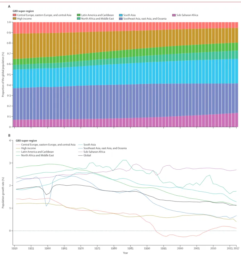
The trend in world population from 1950 to 2017 by

GBD super-region is shown in figure 4. From 1950 to

1980, the global population increased exponentially at an

annualised rate of 1·9% (95% UI 1·88–1·92). From

1981 to 2017, however, the pace of the global

popu-lation increase has been largely linear, increasing by

83·6 million (79·8–87·5) people per year. Over the past

10 years (2007–17), the average annual increase in

population has been by 87·2 million (80·8–93·2) people,

compared with 81·5 million (79·0–84·5) people per year

in the previous 10 years (1997–2007). The global

population increased by 197·2% (95% UI 193·3–200·8),

from 2·6 billion (2·5–2·6) people in 1950 to 7·6 billion

(7·4–7·9) people in 2017. Over this period, the

composition of the world’s population changed

substantially. In 1950, the high-income, central Europe,

eastern Europe, and central Asia GBD super-regions

accounted for 35·2% of the global population but, in

2017, the populations of these countries accounted for

19·5% of the global population. Large increases occurred

in the proportion of the world’s population living in

south Asia, sub-Saharan Africa, Latin America and

the Caribbean, and north Africa and the Middle East.

The annual population growth rate between 1950 and

2017, globally and for the GBD super-regions, is shown

in figure 4. Growth of the global population increased

in the 1950s and reached 2·0% per year in 1964, then

slowly decreased to 1·1% in 2017. The slow shift in the

global population growth rate is determined by

markedly different trends by super-region. Growth of

the popu lation in north Africa and the Middle East

increased until the 1970s, and it has remained quite

high, at 1·7% in 2017. Population growth rates in

sub-Saharan Africa increased from 1950 to 1985, decreased

during 1985–1993, increased again until 1997, and then

plateaued; at 2·7% in 2017, population growth rates

were almost the highest rates ever recorded in this

region. The most substantial changes to population

growth rates were in the southeast Asia, east Asia, and

Oceania super-region, where the population growth

rate decreased from 2·5% in 1963 to 0·7% in 2017. The

large reduction in the population growth rate for this

super-region around 1960 was due to the Great Leap

Forward in China. In central Europe, eastern Europe,

and central Asia, the population growth rate dropped

rapidly after 1987 and was negative from 1993 to 2008.

Growth rates in the high-income super-region have

changed the least, starting at 1·2% in 1950 and reaching

0·4% in 2017.

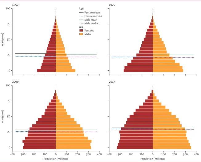
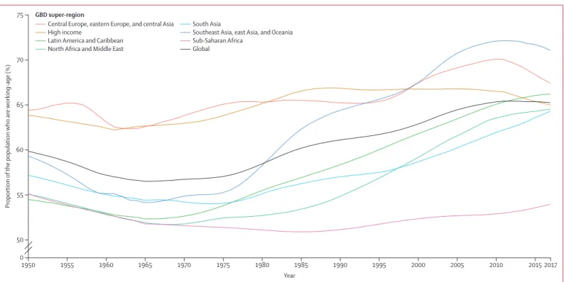
Global population pyramids in 1950, 1975, 2000, and

2017 are shown in figure 5. As the world’s population

has grown, not only has the distribution of the global

population shifted toward sub-Saharan Africa and

south Asia, but the age structure of the global population

has also changed considerably. In 1950, the global mean

age of a person was 26·6 years, decreasing to 26·0 years,

in 1975, then increasing to 29·0 years in 2000 and

32·1 years in 2017. Demographic change has economic

consequences, and the proportion of the population that

(13)

is of working age (15–64 years) decreased from 59·9% in

1950 to 57·1% in 1975, then increased to 62·9% in 2000

and 65·3% in 2017. Another dimension of the global

population is the proportion of the population that is

female, which decreased from 50·1% to 49·8% over the

67-year period.

1950 1955 1960 1965 1970 1975 1980 1985 1990 1995 2000 2005 2010 2015 2017 0 1 2 4 3

Population growth rate (%)

Year

B

0 0·1 0·2 0·3 0·4 0·5 0·6 0·7 0·8 0·9 1·0 Proportion of

the global population (%)

A

GBD super-region

Central Europe, eastern Europe, and central Asia

High income Latin America and CaribbeanNorth Africa and Middle East South AsiaSoutheast Asia, east Asia, and Oceania Sub-Saharan Africa

GBD super-region

Central Europe, eastern Europe, and central Asia High income

Latin America and Caribbean North Africa and Middle East

South Asia

Southeast Asia, east Asia, and Oceania Sub-Saharan Africa

Global

Figure 4: Proportion of the global population accounted for by the GBD super-regions (A) and the annual population growth rates, globally and for the super-regions (B)

(14)

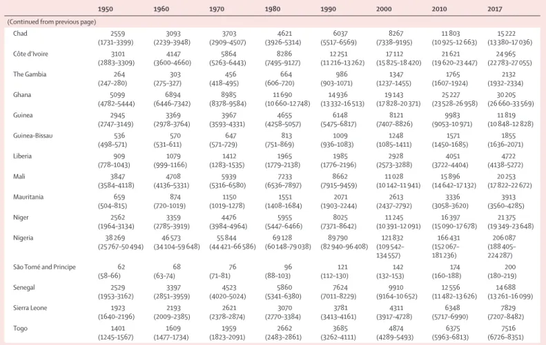
National

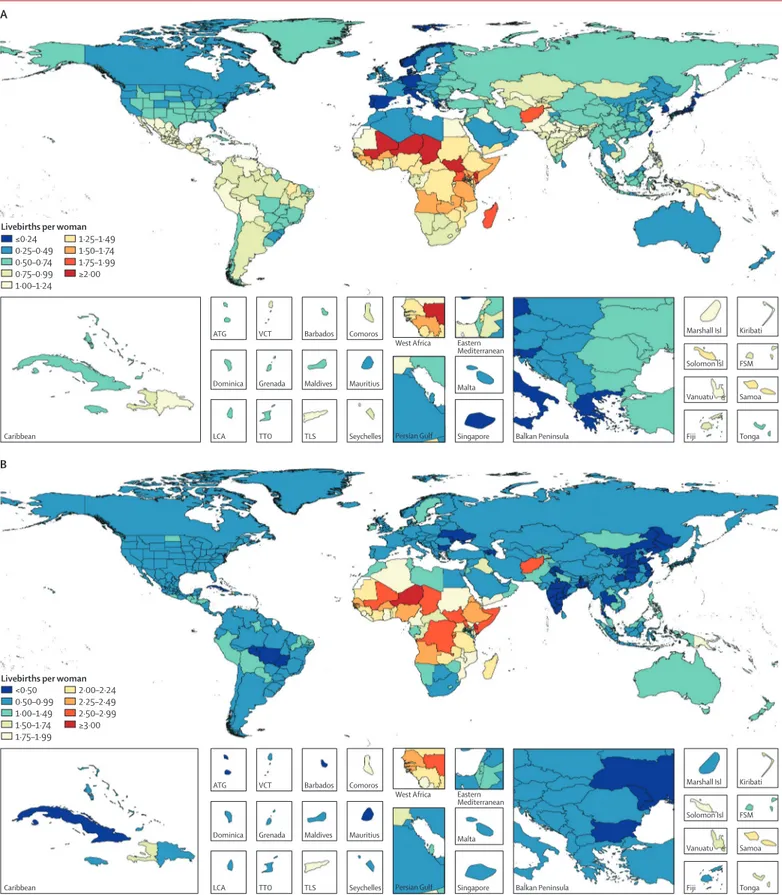
Fertility rates vary substantially across countries and

over time (table 1; appendix 2). In 1950, TFR ranged

from a low of 1·7 livebirths (95% UI 1·4–2·0) in Andorra

to a high of 8·9 livebirths (8·7–9·0) in Jordan. The TFR

decreased in all 195 countries and territories between

1950 and 2017, and 102 countries and territories showed

a decrease of more than 50%. By 2017, the TFR ranged

from a low of 1·0 livebirths (0·9–1·2) in Cyprus to a

high of 7·1 livebirths (6·8–7·4) in Niger. Although a

useful summary, the TFR masks variation in trends in

fertility at different ages in many countries. The global

decrease in median ASFRs from 1950 to 2017 was

43·4% in women aged 15–19 years and 49·4% in women

aged 20–24 years, which contrasts with the observed

decreases in the median ASFR in older age groups of

mothers of 59·4% in women aged 40–44 years, 65·6% in

women aged 45–49 years, and 68·7% in women aged

50–54 years.

In 2017, the TFU25 ranged from 0·08 livebirths

(95% UI 0·07–0·09) in South Korea to 2·4 livebirths

(2·2–2·6) in Niger (figure 6), which is 31 times higher.

Countries and territories where the TFU25 was

less than 0·25 livebirths included many in western

Europe, Japan, South Korea, and Taiwan (province of

China). TFU25 exceeded 1·5 livebirths in many parts

of western, eastern, and central sub-Saharan Africa and

in Afghanistan. Trends in TFO30 are more complex;

decreases in fertility rate are observed at earlier stages of

development, and there are sustained increases in

fertility rate at higher levels of development due to

women delaying childbearing. TFO30 ranged from a

low of 0·3 livebirths (0·3–0·4) in Puerto Rico to a high

of 3·1 livebirths (3·0–3·2) in Niger. In 2017, 145 countries

showed higher fertility in women older than 30 years

than in women younger than 25 years. The geographical

pattern shows low fertility in women older than 30 years

in disparate settings: central and eastern Europe, China,

India, many parts of Latin America, and in some parts

of the Middle East. North America, western Europe,

central Europe, eastern Europe, Australasia, and

high-income Asia Pacific had a higher TFO30 in 2017 than

in 1975, with a mean

of 60·2% higher TFO30 in

these regions.

Figure 7 shows the areas where the TFO30 has

been increasing since 1975; increases of more than

Females Males Female mean Female median Male mean Male median Age Sex 400 300 200 100 0 100 200 300 400 0 25 50 75 100 Age (years) Population (millions) 400 300 200 100 0 100 200 300 400 Population (millions) 2000 2017 0 25 50 75 100 Age (years) 1950 1975