Efficiency of Foreign Debt Portfolio Management in Emerging Economies

Efficiency of Foreign Debt

Portfolio Management in

Emerging Economies

Bachelor Thesis in Economics

The Department of Economics, Finance and Statistics Jönköping International Business School

Author: Sapto Adinugrahan, Mochamad Ridwan Tutor: Kristofer Månsson

Title: Efficiency of Foreign Debt Portfolio Management in Emerging Economies

Author: Sapto Adinugrahan

sapto_adinugrahan@yahoo.co.uk

Mochamad Ridwan

mcridwan@aol.com

Tutor: Kristofer Månsson

Date: 2015-05-11

Subject terms: Public debt management; Foreign debt portfolio; Exchange rate ex-posure; Emerging economies; Currency composition

JEL classification: C22, F34, H63

Abstract

Fluctuation of exchange rate has affected the increasing burden of foreign debt payment in emerging economies. This issue has negatively influenced the economic growth. It has been a severe obstacle considering that governments have to issue public debt denomi-nated in foreign currency to finance the budget deficit. Hence, there is an urgent necessity to implement an efficient public debt management to minimize the exchange rate expo-sure. This thesis analyses how efficient the foreign debt portfolio management is in the 14 emerging economies under examination in the period of 1990-2013. Panel Dynamic Fixed-effect Estimator and Granger Causality approach are applied to analyze how re-sponsive the currency composition of foreign debt portfolio to the exchange rates move-ment. The thesis examines the four biggest foreign debt shares that are denominated in US dollar, Euro, British pound, and Japanese yen, and the related exchange rates move-ment in the economies under consideration. The observation concludes that the foreign debt portfolio management in these emerging economies is not efficient or not optimal. The evidences prove that changes in the exchange rates of Euro, British pound, and Jap-anese yen relative to US dollar Granger cause changes in respected debt shares. It means that there is no substitution effects from the appreciation of the currencies vis-à-vis the US dollar during the year of observation.

Table of Contents

1

INTRODUCTION ... 1

2

BACKGROUND ... 4

3

THEORY ... 8

3.1 Portfolio Theory Development ... 8

3.2 Hypothesis ... 12

3.3 Causes of Inefficiency in Foreign Debt Portfolio ... 13

4

METHOD ... 16

4.1 Unit Root Testing ... 16

4.2 Cointegration Testing ... 16

4.3 Cointegrating Vectors in Panels and Reversal Time ... 17

5

DATA AND RESULTS... 19

5.1 Data and Preliminary Findings ... 19

5.2 Panel Unit Root Testing ... 22

5.3 Cointegration Testing ... 22

5.4 Cointegrating Vectors in Panels and Reversal Time ... 23

6

ANALYSIS ... 26

6.1 Preliminary Findings Analysis ... 26

6.2 Econometrics Model Analysis ... 26

6.3 Economic Analysis ... 28

7

CONCLUSIONS ... 31

Figures

Figure 1 Efficient frontier and cost-at-risk (CaR) ... 11

Figure 2 Foreign Currency-denominated Debt Shares and Exchange Rates ... 20

Tables

Table 2 Preliminary Test ... 21

Table 3 Unit Root Test ... 22

Table 4 Panel Cointegration Test (Pedroni (Engle-Granger based)) ... 22

Table 5 Panel Cointegration Test (Kao (Engle-Granger based)) ... 22

Table 6 Dynamic Fixed-effect Estimator (DFE) ... 23

Table 7 Reversal Time ... 24

No table of figures entries found.

Acknowledgment

This thesis was supported by Swedish Institute. We thank our supervisor, Kristofer Månsson, for supervision with advices in Econometrics Views and for comments that greatly improved the thesis.

Sapto Adinugrahan would like to show gratitude to A. Cleton for supporting by any means during the studies as well as Mr. Karel Brůna for advices on literatures, and to dedicate the work to N. Qurrata Aini. Mochamad Ridwan would like to show gratitude to Professor Andreas Stephan for the knowledge gained of Optimal Portfolio Choice and the Capital Asset Pricing Model and Professor Scott Hacker for the knowledge gained of Econometrics and Exchange Rate Volatility.

Sapto Adinugrahan Mochamad Ridwan

1

INTRODUCTION

This thesis investigates how efficient the foreign debt portfolio management is in the selected 14 emerging economies i.e. Brazil, China, Colombia, Egypt, Hungary, India, Indonesia, Ma-laysia, Mexico, Morocco, Peru, Philippines, Thailand, and Turkey from 1990-2013. This issue has become substantial since the vulnerability of exchange rate has increased the debt burden in emerging economies. Hence, it is essential to analyze how efficient foreign debt portfolio management is in emerging economies considering that they have different characteristics as developed economies.

In order to assess the efficiency of the foreign debt portfolio, the model used in this thesis examine the debt shares denominated in US dollar, Euro, British pound, and Japanese yen and corresponding exchange rates i.e. EUR/USD, GBP/USD and JPY/USD from 1990-2013. The main finding of the thesis is that the foreign debt portfolio management is not efficient. Fur-thermore, the result shows that there is no substitution effect i.e. changes in volume of respected debt shares relative to debt shares denominated in US dollar to cancel out the changes of US dollar value of debt shares denominated in Euro, British pound, and Japanese yen.

1.1 Background

Government debt also known as public debt, national debt, and sovereign debt has a long his-tory. In the past, government issued public debt for funding of battle and other extraordinary activities. Nowadays public debt have been used for more peaceable activities, such as “invest-ments, health care, education and communication systems and the establishment of a social security system” (Public Debt Net, 2015).

Government debt has two categories i.e. internal and external debt. Debtors such as foreign governments, foreign corporations, and international financial institutions can owe external debt or foreign debt. External debt flows through Development Aid e.g. Official Development Assistance (ODA), Foreign Direct Investment (FDI), and Sovereign Bond in terms of emerging economies as debtors.

External debt is outstanding liability that requires payment of principal and interest by the debt-ors. The debtors will pay the principal and interest in the future. Debtors, in this case the gov-ernment, owe the debt to non-residents of an economy. Foreign currency debt is denominated in a currency other than domestic currency but with amounts to be paid linked to a domestic currency or in domestic currency but with the amounts to be paid linked to a foreign currency (International Monetary Fund, 2003).

Foreign exchange exposure has evolved over financial transactions with adverse effect of the exchange rate of the denomination currency in relation to the base currency before the date of maturity. Depreciation of domestic currency can increase the burden of foreign currency debt for the debtors. Furthermore, payments on foreign currency debt can cause downward pressure on domestic exchange rate and or outflows of foreign currency from the economy (International Monetary Fund, 2003).

1.2 Problem

Nowadays, emerging economies that rely heavily on foreign currency debt experience im-portant fiscal policy strategy that challenge on how to manage the exchange rate, interest rate

and maturity associated with the debt. If any of emerging economies are economically success-ful in developing the economic growth, their progress will spur to the neighboring countries. Conversely, if they experience an economic crisis, they have the capacity to bring down their neighboring countries. Emerging economies are the key roles in the future development of world trade, global financial stability, and the alteration to free market economies in Asia, Cen-tral Europe, and Latin America (Garten, 1997).

Mostly the selected emerging economies are associated to BRIICS (Brazil, Russia, India, Indo-nesia, China, and South Africa) that is term used by Organization for Economic Co-operation and Development (OECD) and members of Newly Industrialized Countries (NIC). Emerging economies suffer from the increasing of foreign debt burden due to vulnerability of the ex-change rate of currency of the debt denomination. It has been challenging for debt managers in emerging economies to manage the foreign debt portfolio efficiently over time. This is due to some inflexibilities and drawbacks in emerging economies.

Pegging the debt to one currency, for instance US dollar caused by common foreign trade pat-tern, and creditors that require the debt denominated in their currencies cause inflexibility for debtors to alter the currency composition of the debt when it is needed e.g. when there is ap-preciation of currency of the debt denomination. In addition, the lack of foreign exchange and money market restricts the development of derivatives industry. Derivatives are important in-struments to hedge the debt from exposure of exchange rate and interest rate risks. Although currency composition is one strategy of hedging i.e. choosing the optimal currency composition during the issuance of foreign debt, but keeping the chosen currency composition in an optimal portfolio to stay constant over time is crucial. Based on the situations in the emerging econo-mies described above we would like to assess the recent development on foreign debt portfolio management in emerging economies. Hence, our thesis research question is:

How efficient is the foreign debt portfolio management in emerging economies?

Hussein and de Mello Jr. (2001) studied the same research question for 14 emerging economies i.e. Argentina, Brazil, Chile, Colombia, Egypt, India, Indonesia, South Korea, Malaysia, Mex-ico, Thailand, Philippines, Turkey, and Venezuela for time span of 1970-1998. Their study indicates that foreign debt portfolio management in emerging economies has not been optimal (sub-optimal). They found that changes in exchange rates Granger cause changes in debt shares.

1.3 Purpose

The purpose of the thesis is to evaluate whether foreign debt portfolio management in selected emerging economies has been managed efficient or optimal over time. The method is to address whether currency composition of foreign debt in the selected emerging economies has offset the exchange rate movements. Pooled data and panel unit root test developed by Im, Pesaran, and Shin (1997) was applied for unit root test. Test of cointegration in panel data was conducted using the procedure suggested by Pedroni and Kao (1999).

The long-run relationships between debt shares and the related exchange rates were estimated using the DFE estimator by Pesaran and Shin (1997), and then test whether changes in exchange rate Granger cause changes in debt shares. If changes in debt shares cointegrate with changes in exchange rate, a stable long-run relationship is estimated to be present between changes in the currency composition of a country’s foreign debt portfolio and exchange rate movements. In addition, Granger cause tests a causality relationship between the variables i.e. changes in

exchange rates do Granger cause change in debt shares. According to Hussein and de Mello Jr. (2001) debt portfolio management can be deemed optimal if changes in exchange rates do not Granger cause changes in debt shares denominated in the corresponding currencies.

The study by Hussein and de Mello Jr. (2001) above examines the issue for the year of 1970-1998. However, this thesis will use the data for the year of 1990-2013 to reflect the current development in foreign debt portfolio. This is due to the latest development, for instance, the integration of European countries that use Euro as the currency within Eurozone has affected the currency composition of debt denomination in emerging economies. Besides, their research used Deutsche mark (DM) that is not relevant anymore with the current issue. Hence, this thesis will fill the gap to present the current economic development and current currencies used.

2

BACKGROUND

Public debt management is an open market operation performed by a government to change the composition of its outstanding stock of government-issued debt instruments with the aim e.g. minimizing the cost of public debt, and as a part of economic policy making, for instance for stabilization and for attracting investors (Paalzow, 1992). Here, the focus is only in the compo-sition i.e. the different debt maturity, types, yields, and currency denomination. However, the scope of public debt management has been widened not only for composition changes but also for its size changes.

IMF (2001) in its guidelines for public debt management emphasizes that the main objective of public debt management is to guarantee that the government’s financing needs and the payment obligations are encountered at the lowest possible cost in the medium and long-run term. It is expected that the lowest possible cost is coherent with a sensible level of risk. To achieve this lowest possible cost, a trade-off between acquiring lowest debt-service-cost and risks must be performed.

Furthermore, the fluctuation of exchange rate should also be considered because public debt is not only denominated in domestic currency but also foreign currency. In addition, debt share is also needed to be adjusted in order to have an optimal public debt management. Adjusting the currency composition and debt share has an objective of minimizing government’s debt-ser-vice-cost. This is then why a portfolio approach in public debt management has become im-portant in the recent years.

2.1 Literature

The very early literature about modern portfolio is the idea from Markowitz (1952) who states that the process of selecting portfolio consists of two stages. First stage is observation about the available securities, and second relevant believe about future performance of the securities then end it with choice of portfolio. He formulated that portfolio is a problem of choice of the mean and variance of a portfolio assets. Markowitz idea originates the modern portfolio theory. Furthermore, Tobin (1958) develops an early work on modern portfolio theory. He states that the optimal portfolio management is held by optimality of return distribution or utility function by balancing both riskless assets and risky assets. In addition, Sharpe (1964) completes the model by introducing an equilibrium position in the capital market for an optimal portfolio. A more comprehensive discussion about it is presented in Chapter 3 along with the works from Hahm and Kim (2003) and Kroner and Claessens (1991) for an optimal public debt portfolio. Literatures in public debt management have gained interest in the last two decades since the need of public debt has been increased. In the beginning of 1990s, the literatures in public debt management focused in debt reduction or forgiveness for poor countries as the result of Toronto Summit in 1988 (Raffer, 2010). He mentioned that this era ended the illiquidity theory that believed that the debt problem was not caused by fundamental crisis but only by the inability of poor countries to repay their debts, in fact it was the opposite.

A fundamental crisis case from emerging economy related to increasing of public debt was the Mexico crisis that happened in 1994-95. The country’s political instability and of imposing expansionary fiscal and monetary policy has triggered the crisis. Issuing public debt denomi-nated in US dollar to buy Mexican peso caused speculation on overvalue of Mexican peso which then causing investors to move capital out from Mexico to United States. The devaluation

of Mexican peso triggered increasing risk-premium from investors and causing the hyperinfla-tion which at the end caused Mexico to default. This “Tequila” crisis then spread to Asia and the other Latin America economies (The Economist, 2014).

Another fundamental crisis was Thailand crisis in 1997-98 that triggered by floating of Bath by Bank of Thailand has spill-overed and collapsed the economies in the region. Among other things, the regime of fixed or semi fixed exchange rate in Thailand, Indonesia, and South Korea and the vulnerability of economies because investors who held the public debt were located in foreign countries created huge exchange rate exposure causing these three economies the most severe impact in this Asian financial crisis (The Economist, 2007).

The investors’ weak confidence spill-overed by Asian financial crisis and the fragile fundamen-tal of domestic economy caused Russian crisis in 1998 that then ended the fixed exchange rate regime in the country. Increasing interest rate, fears of Russian ruble devaluation and default on Russian ruble denominated public debt collapsed the stock, bond, and currency markets. The yield on bond rose to more than 200% and stock price fell sharply amounted to 70% of the value forcing the Bank of Russia to let the Russian ruble to floating (Rabobank, 2013). The other remarkable financial crisis was Brazil and Ecuador crisis in 1999. Ecuador performed debt rescheduling/restructuring in 1999-2000 and declared default.

In the late 1990s, the public debt management focused more on market–oriented reform, which emphasized on liberalization of trade, investment, and facilitating international capital move-ments (International Monetary Fund, 1998). These policies are a part of ten agendas of Wash-ington Consensus as “new economic order” promoted by IMF, World Bank, Inter-American Development Bank, and U.S. Treasury from Washington DC for pursuing a global free market. Argentina that implemented the convertibility law, one Argentine peso for one US dollar, had to undergo depreciation of Argentine peso later to 0.25 Argentine peso for one US dollar. It caused a fall in Gross Domestic Product (GDP) in term of US dollar. Argentina lost its product competitiveness after Brazil, Argentina’s export competitor, devalued its currency. This brought Argentina to a financial crisis in 2001 and forced it to ask for debt rescheduling/re-structuring.

In the beginning of 2000, the literature in public debt management focused more in debt re-structuring for sustainable public debt. Raffer (2010) stated that in November 2001, IMF started to advocate the idea -which it used to oppose before- of sovereign insolvency by introducing Sovereign Debt Restructuring Mechanism (SDRM). This idea requires a sufficient amount of debt reduction to reach a sustainable public debt for typical emerging economies, which is only about 25 percent of GDP. While the idea of illiquidity is more to short term inability to repay debt, the insolvency is more of long term inability to repay the debt caused by too low of reve-nue or economic capacity which it is closer to the concept of default.

In 2005, literature in public debt management progressed to a further issue concerning a deeper debt relief. The creditor countries took a further step in this issue, including Norway that pro-posed the idea of Multilateral Debt Relief Initiative (MDRI) in which illegitimate debt, that then the characteristics had to be determine by the United Nation, must be cancelled. The relief was intended to enable the debtor’s countries to meet their current and future external debt-service and to reach Millennium Development Goals (MDGs) (Raffer, 2010).

In the late 2000s, the literature in public debt management focused more on how to achieve a sustainable public debt (Greiner & Fincke, 2009). Countries including emerging economies

have issued more debt to counter the deficit especially after the financial crisis in 2008. The flow of international capital has been hugely increased more than previous years and investors search for higher return. Not only in developing countries, public debt in developed countries has also shown a growing trend. It is caused by the practice of budget deficit, where the gov-ernment spending is more than the revenue, and to finance the deficit issuing public debt is a sound alternative.

The recent development shows a largely increasing the practice of derivatives as hedging in-struments in public debt. It has shifted the focus of literature in public debt management to foreign debt portfolio management. In addition, the international capital flow interconnects countries since the creditors of public debt in emerging economies are usually institutional from foreign countries and so the debt are issued denominated in foreign currency. Hence, many countries have changed their foreign debt portfolio both in the size and currency composition as a further concern in public debt management (IMF; Bank, World, 2014).

2.2 Previous Studies

Researchers have conducted studies on assessing the optimal foreign debt portfolio manage-ment in emerging economies. Demirguc–Kunt and Detrigiache (1994) exercised nine highly indebted countries i.e. Argentina, Indonesia, Philippines, Brazil, South Korea, Venezuela, Chile, Mexico, and Turkey for the year of 1973-89. They argue that the countries should focus on interest payment since during debt crises bank are hesitant to reschedule interest payment, while principal rescheduling is almost a usual event. Different behaviors from creditors by im-posing lower interest rate on loans for Asian countries has decreased the debt burden in Asian countries compared to Latin American countries. Creditors subsidize a lower interest rate since the default risk spread is lower. Large growth of Gross National Product (GNP), low ratios of imports to GNP, and large share of official debt initiated lower spreads.

Dooley (2000) discovers that debt management policy in industrial countries is not relevant for developing countries because minimizing debt-service-cost will increase the cost of default. Default is not relevant for industrial countries therefore they do not bear this risk. Hence, he suggests that minimizing debt service costs is not efficient for emerging economies since lacks many of the financial markets that private sector cannot fully offset the government financial position regarding its assets and liabilities.

He also states that changes in the government’s balance sheet are neutral, and under the as-sumptions, the private sector would fully offset any financial position the government take (Dooley, 2000). Choosing an efficient frontier for assets and debt portfolio as a usual practice in corporate finance implicitly ignores default risk. This issue has not been widely applied in sovereign finance. Industrial countries can choose or force to default in an efficient frontier but for developing countries, this cost of default is too high to undertake.

Hussein and de Mello Jr. (2001) examined 14 emerging economies i.e. Argentina, Brazil, Chile, Colombia, Egypt, India, Indonesia, South Korea, Malaysia, Mexico, Thailand, Philippines, Tur-key, and Venezuela for the year of 1970–1998. They concluded that these countries foreign debt portfolio management had been sub–optimal (not optimal). They exercised the debt shares denominated in US dollar, Deutsche mark (DM), Japanese yen, and Swiss francs and their re-lationship with respected exchange rates.

The study performed by Hussein and de Mello Jr. (2001) shows a more recent development in the issue of efficiency on foreign debt portfolio management. While Dooley focused more, on the theory whether emerging economies could perform an efficient portfolio or not, Hussein and de Mello Jr. examined directly the fact about what emerging economies had achieved in the years under consideration.

Emerging economies, nevertheless, will always encounter the risk of default. The question is then how to avoid that risk with an optimal portfolio management, and several policies in avoid-ing exposure to the foreign debt for instance usavoid-ing derivative i.e. forwards contract, futures contract, currency and interest rate swap, and option as hedging policy. Applying an optimal foreign debt portfolio management and other financial policy in debt management will certainly can bring emerging economies to an efficient foreign debt portfolio management and able to avoid default risk.

3

THEORY

The theory of debt portfolio is an adaptation from theory of investment portfolio. The develop-ment of modern portfolio theory started in the 1990s by several economists. In this section, the ideas from several economists that have contributed to the development of modern portfolio theory are presented such as Harry Markowitz (1952); James Tobin (1958); and William J. Sharpe (1964).

Debt managers in country level and researchers have tried to formulate the most appropriate approach in the adapting the investment portfolio to debt portfolio. It has resulted in different approaches. The investment theory, which is in demand side, consisting of investors and cred-itors has to be adapted to supply side consisting of debtors. These two sides modification has been challenging since the investment portfolio theory is for private sector, while its application for public debt management has not been sufficient. This is because a government asset - na-tional tax, for instance is not in the form of financial asset.

However, the ultimate goal of debt portfolio management is still the same between private and public sector that is minimizing the cost of borrowing given the trade-off between expected debt-service-costs and risks associated with various borrowing strategies (Hahm and Kim, 2003). In this thesis, an approach from Kroner and Claessens (1991) is also presented. Their study analyzes how a country should choose the currency composition for an optimal foreign debt portfolio. In addition, a study by Hahm and Kim (2003) for an efficient debt portfolio using the concept of cost-at-risk (CaR) which is an adaptation of value-at-risk (VaR) in general is presented.

3.1 Portfolio Theory Development

Markowitz (1952) on his theory on portfolio selection states that to execute the choice of a portfolio process investor will maximize the discounted value of future returns (E) and mini-mize variance (V). This combination of securities, which reflect a diversification in the portfo-lio, resulted in maximum expected return with minimum variance (E-V rule) then defines as an efficient portfolio.

Markowitz argues that the model should use covariance instead of variance to reflect the overall securities in the portfolio. Applying this method to debt portfolio, means that return for the investor and or creditors is the cost for debtors. Since investors/creditors will choose the effi-cient frontier of portfolio available in the market therefore debtors has to trade off the cost of borrowing (return for investors/creditors) and risk of issuing debt (covariance of the overall securities).

Tobin (1958) develops Markowitz theory by introducing riskless asset to a portfolio. He argues that investors prefer to hold cash investment with yield of zero (assumed to be riskless invest-ment), for liquidity reason and risk-avoiding behavior, and investing in yielding investments. Investors can analyze the future probability of the portfolio by deriving indifference curves from combinations of expected returns and risks (standard deviation) on non-yielding and yield-ing investments with different interest rates. So first, investor has to choose yieldyield-ing invest-ments and then second, combining that basket of investinvest-ments with a riskless investment. Yielding investments (or risky investments) can be a composite of investments e.g. bonds and other debt instruments differing in maturities, debtors, and other features. Hence, investors will maximize the utility function of the future probabilities. The optimum portfolio is then defined

as the highest possible expectation of return available to investors at level of risks; then it is called as dominant pairs of investment combinations. A balance of combination between risk-less investment and risky investments constructs the dominant pairs.

A risk-free rate investment in a portfolio theory can diversify away the risk on the portfolio arising from risky investments. The efficient portfolio provided by the efficient frontier line then nowadays called as the capital market line. In the term of debt portfolio, the debtors then pursue issuing riskless securities e.g. treasury bills so that the market can generate the market efficient frontier available to the investors. The debtors’ task is then to manage the trade-off between cost of borrowing (return for the investors) and risk (standard deviation or covariance). Sharpe (1964) points out that the two theories above do not reveal the market equilibrium under uncertainty. He argues the effect of an investment on an investor’s over-all investment oppor-tunity risk depends not only to the expected return and risk, but also to its correlation with other available investments. The condition where correlation is considered in determining probabili-ties of expected returns and risks must be hold in equilibrium.

Sharpe model is an improvement of Markowitz and Tobin theories. He states that assets (in-vestments) price will cause investors’ actions with “new combination or combination become attractive”. This process further will change the asset prices until all assets lying in capital mar-ket line. This is the equilibrium condition where there is simple linear relationship between expected return and standard deviation for efficient combination in the risky assets. This rela-tionship is consistent or then called as systematic risk. On the other hand, there is a part of an asset’s risk that is due to its correlation with the return on combination cannot be diversified away when asset is added to the combination. Two combinations of assets will be tangent in an equilibrium.

The expected rate of return of investing in riskless asset and some risky assets is derived as:

Ra Rp

Rc aE a E

E  (1 ) (1)

ERc corresponds to expected rate of return on investing in riskless and risky assets, ERp is riskless

interest rate, Era is expected rate of return on risky assets, a is proportion of fund invested in

riskless asset, and 1-a is remainder proportion of fund invested in risky asset. The standard deviation of a combination of investments is:

σ

σ

σ

σ

σ

These three developments of portfolio model above have been used nowadays in assessing and managing risk. The concept is used for both asset position and liability position by using value at risk. Value here can be value of assets/investment or value of debt which are estimated to be at risk.

Sharpe also mentions that by holding the position on assets and liabilities the concept of Capital Asset Pricing Model (CAPM) can be applied. Assets and liabilities can be denominated in do-mestic and foreign currency; and for the latter the exposure of risk is higher coming from fluc-tuation of foreign exchange rate. This is also a concern for debt agency in managing the risks. To summarize, the theory on portfolio shows a development in the portfolio theory where Mar-kowitz introduces a portfolio consisting of combination of different investments by trading-off

the overall returns and risks. Tobin introduces risk-free rate investment to the portfolio con-structed by Markowitz, and then Sharpe completes the model by introducing correlation in de-termining the optimal portfolio from Tobin model.

Furthermore, in choosing an optimal currency composition of foreign debt, Kroner and Claessens (1991) relate the exchange rates to commodity price. A country’s pattern of trade will affect the currency denomination of export revenue that relates to which its exchange rate is managed. They argue that this approach reflects the currency composition choice for a con-tinuous time portfolio model. Intuitively, a country “seeks to minimize the variability of its debt service relative to a measure of its foregone consumptions” (Kroner & Claessens 1991, p.134). They state that an optimal risk-minimizing in term of currency composition defined by a func-tion of the condifunc-tional covariance of the exchange rate depreciafunc-tions and the condifunc-tional covar-iance of each of the exchange rate depreciation with the price variable, shown in the following model:

b*(S,t)=yy(S,t)-1yp(S,t) (3)

b*(S,t) corresponds to an optimal holding of foreign bonds, yy(S,t) is conditional covariance

matrix of exchange rate depreciations, and yp(S,t) is the matrix of conditional covariance

be-tween the exchange rate depreciations and percentage changes in the price variable. A positive elements of vector b*(S,t) indicate an optimal borrowing shares, on the other hand a negative elements indicates asset share. The resulting borrowing shares correspond to the country’s net foreign liabilities which is gross debt minus foreign exchange reserve (Kroner and Claessens, 1991).

Hahm and Kim (2003) argue that Asset-Liability Management (ALM) framework is not widely adopted since differences between private and public sector. For this reason, they state that the actual practice of debt management is partial measures such as durations for interest rate risks and maturities for liquidity risks. Hence, they implement the concept of cost-at-risk (CaR) to identify a target benchmark portfolio. The efficient portfolio is then defined as a trade-off be-tween the mean and volatility of debt-service-cost. It is the main concern of a government debt agency. Debt-service-cost depends on interest payment and principal (issuance) of debt up to a certain year. To control debt-service-cost, a natural risk can be targeted using cost-at-risk. Cost-at-risk is the maximum possible yearly interest cost that can be realized in a given year at a given confidence interval, for instance 95%, as shown in the following model:

CaR= μ + 1.645σ (4)

μ= CaR-1.645σ (5)

CaR represents maximum tolerable interest cost, μ is expected value of annual debt-service-cost, and σ is standard deviation of annual debt-service-cost. It shows that cost-at-risk is repre-sented as a downward sloping line with slope of -1.645 in the plane of expected value and standard deviation of annual debt-service-cost. Then the relationship between expected cost (at 95% CaR) and risk (standard deviation) is shown in the following figure:

Figure 1 Efficient frontier and cost-at-risk (CaR)

Source: Hahm and Kim (2003),Cost-at-risk and benchmark government debt portfolio in Korea, p.89

From the above figure, the efficient frontier is shown by a downward sloping curve where only debt portfolio above the curve can be obtained. Suppose a government applies a 95% CaR at CaR1. The feasible portfolio is one where it is located under the CaR1 line therefore portfolio B

and C are feasible, while A is not feasible. By obtaining the weighted average of deviations and minimizing 95% CaR, we can identify the benchmark at CaR* at portfolio B where CaR* line tangent to the efficient frontier.

The theories on portfolio described above show how investors and debtors deal with choosing the right combination for an optimal portfolio. However, it does not show how to keep the chosen portfolio to stay constant over time. When the time change, there is risk of exposure arise from changes in exchange rate. This exchange rate exposure is also important for debt agency to handle if the government wants to hedge the debt using an optimal currency compo-sition.

Due to above reason, this thesis focuses to examine how to take the next step, keeping the chosen optimal currency composition in the debt portfolio unchanged by keeping the value of debt share constant. Hence, this thesis applies the procedure proposed by Hussein and de Mello Jr. (2001) for assessing whether debt managers have kept the US dollar value of debt shares constant, stay in the optimal foreign debt portfolio.

3.2 Hypothesis

As stated above that there have been attempts from researchers and government debt agencies to formulate the approach for choosing securities for an optimal foreign debt portfolio. In this thesis, we will not discuss on how to choose the debt securities for an optimal portfolio but we will analyze how to keep an optimal chosen portfolio constant over time. Since the exposure of exchange rate is crucial to a debt portfolio, therefore we analyze the foreign debt portfolio by relating the exchange rate movements with debt shares.

We assume that debt managers in the emerging economies under consideration have performed the process of choosing an optimal securities. Our focus is then how to maintain this optimal choice of securities unchanged in term of US dollar value of the debt share. For economies with a given existing foreign debt, to keep the value of the debt in portfolio constant (optimal), Hus-sein and de Mello Jr. (2001) examined how emerging economies pursue this strategy. The model they propose can be described in the following discussion.

Suppose that foreign debt of a country is denominated in currency i until currency n. Let that currency n is the numéraire such that exchange rates of currency i (eit where i=1, …. , n-1) is

define by the value of currency i per 1 unit of currency n. In this case, i is Euro, British pound, and Japanese yen whereas n is US dollar.

The objective of the debt agency is to minimize the total value of foreign debt in a portfolio defined by Min Ct (At; Dit), where Ct is portfolio C at time t, At is total foreign assets and Dit is

foreign debt denominated in currency i. Minimizing the total value of foreign debt in a portfolio means that the first derivative should equal to less than zero and the second derivative is equal to more than zero. Minimizing the total value of foreign debt in a portfolio according to Hussein and de Mello Jr. (2001) is:

   n i Ee D D it t it t 1 (6)

Dt represents total value of foreign debt at time t (in US dollar), Dit is debt share denominated

in currency i at time t, Et is the expectation operator, and eit is exchange rate currency i relative

to currency n (US dollar). Standard manipulation of the first-order condition (first derivative) for cost minimization then defines that if currency i is expected to appreciate with respect to currency n (Eteit falls), the effect is that i-denominated debt on portfolio C rises relative to debt

denominated in n; because Ci<0 the share of foreign debt denominated in i, Dit,falls. Hence, the

expected appreciation of currency i relative to currency n implies a fall in the share of debt denominated in i relative to n.

By assuming that Eteit = eit then Dit/Dnt = eit. which means that an appreciation of currency i with

respect to n (a fall in eit) will cause a fall in the debt share denominated in i, relative to debt

share denominated in n. The change in the volume of debt denominated in i relative to n offsets the appreciation of i to keep the n-value of the debt portfolio constant. Hence, the thesis hy-pothesis is:

“In an efficient foreign debt portfolio management, an appreciation of currency i with respect to US dollar (a fall in eit) causes a fall in the debt share denominated in i relative to debt

An example of a case from the above hypothesis is if, for instance, i is Japanese yen (n is US dollar). An appreciation of Japanese yen with respect to US dollar (a fall in JPY/USD exchange rate) causes a fall in the debt share denominated in Japanese yen relative to debt share denom-inated in US dollar to keep the US dollar value of debt share denomdenom-inated in Japanese yen constant. Constant in the US dollar value of debt share denominated in Japanese yen means that the portfolio maintains the optimal value as the first time the debt established.

At the time the debt were established, or we take it as given in this case, we assume that the debt agencies have chosen the currency composition and shares as an optimal currency compo-sition as the theory of portfolio described by Kroner and Claessens (1991). In addition, when the US dollar value of debt share denominated in Japanese yen is constant, according to Hussein and de Mello Jr. (2001) this is an optimal foreign debt portfolio management.

Furthermore, to measure how quickly the after-shock position to get back to the initial or effi-cient position, the method of convergence time based on the dynamic panel model can be ap-plied. The coefficient on the lagged dependent variables i.e. debt share denominated in i in each regression model allows us to do that easily.

3.3 Causes of Inefficiency in Foreign Debt Portfolio

It has been challenging for emerging economies to manage successfully an efficient foreign debt portfolio over time because they exhibit some inflexibilities. These drawbacks reduce the efficiency of foreign debt portfolio management in the emerging economies. A drawback that reduces the efficiency of foreign debt portfolio management is that country’s foreign trade pat-tern that causes the emerging economies peg their currency to mostly US dollar. It causes ina-bility or unwillingness to change the currency composition of the foreign debt to other curren-cies. In addition, for a conventional loan, creditors often require the debt denominated in their currencies which in turn cause inflexibility for debtors to change the currency composition in case that the portion of the debt is needed to be adjusted to reflect appreciation of exchange rates (Hussein & de Mello Jr., 2001).

Furthermore, the infrastructure for foreign exchange and money market in emerging economies is not well-established as in developed economies. A well-established foreign exchange and money market can provide derivatives industry to grow, which is important for debt managers if they want to hedge the foreign debt from exchange rate and interest rate risks. With deriva-tives instruments widely available in the market not only for private but also for public sector, can benefit the debt portfolio management from the exercise of derivatives as hedging strategy. Although currency composition of debt is one strategy that can be categorized as hedging tech-nique, but this is particularly true during the decision of issuing the debt. Since the exchange rate fluctuates over time, another hedging strategy using derivatives is needed to maintain the efficiency of the portfolio, keeping the optimal choice of the portfolio constant over time. According to Bergendahl and Sjögren (2006) to conduct hedging one must do the following steps:

1. Estimate future exposure of a transaction for a relevant set of time

2. Plan to net out with foreign assets denominated in the same currency as much as possible of these exposure

3. The residual (net) exposure is hedged using derivatives with a certain percentage (say 50-75 per cent) of these exposure month by month, one year ahead. The closer to the date of delivery, the more certain the exposure to come

Aggarwal and Demaskey (1997) state, hedging in emerging economies to reduce the currency risk exposure is often difficult or impossible since lack of well-developed derivatives market. Derivatives are financial contracts that obligate counterparties involved to exchange cash pay-ments related to values of a commodity/financial/underlying asset with no actual delivery of those assets (Kohn, 2004). The widespread of exchange rate controls and other regulations in emerging economies restrict the activities in the foreign exchange markets. Although the history of derivative markets started in the early 1980s in U.S. and Europe then spread to Asia in the early 1990s, for instance, but the development of derivative markets in Asia has not been sig-nificant.

This is due to the Asian crisis in 1997 starting with the issue of floating of Thai baht that ham-pered the derivative markets development. During that period, the use of forwards contract and interest and currency swap in local currencies has been initiated (Cooke, 1998). The demand from private sector for hedging instruments in Asia showed an increased after that period. How-ever, the financial crisis in 2008 affected the development of derivatives market for the second time causing the Asian currencies are much vulnerable and not stable. These phases of devel-opment are different with that in U.S. and Europe where there has been good economic condi-tion that provide room for the derivative market to be developed in the early 1980s.

There have been drawbacks why foreign exchange and money market have not been developed as good as the counterparty in U.S. and Europe. Cooke (1998) points out that, there are three factors that drawback the development i.e. the restricted convertibility of Asian currencies im-posing strong regulatory control for domestic derivatives, the floating rate definition, and type of derivatives instrument.

Asian currencies have been pegged to a certain foreign currency e.g. US dollar and restricted in convertibility to other currencies. All derivatives products first become available offshore (no foreign currency market in domestic countries) in non-deliverable form, not only Non-De-liverable-Forward but also for currency and interest rate swap. In order to have room for devel-opment, an onshore (foreign currency market in domestic countries) deliverable market for in-terest rate and currency swap is needed. The controls on domestic market cause banks hesitant to get involved in the market and avoid potential effect on their domestic relationship with government authorities e.g. Singapore that controls exercised on the domestic use of its cur-rency derivative.

Derivatives industry needs a floating rate that independently determined available online daily on a screen for showing cost to potential hedging customers. However, these requirements are not supported by Asian countries e.g. floating rate lending in Thai baht is conducted by banks based on individual minimum lending rate.

The types of instruments available in Asian derivatives market are not as many as in U.S. and Europe. Initially forwards contract and cross currency swap are available. Other than that, they are not available. Although type of instruments will be available in the future, the regulation of using hedging in public sector need to be adapted from private sector.

An example of lack of regulation for allowing public sector to enter derivative market is Indo-nesia that categorizes any events that cause a loss to the state budget is a corruption. Hence,

debt managers in the public sector are hesitant to conduct hedging practice due to severe pun-ishment of committing a loss from hedging that means a corruption. However, there has been a significant progress towards public sector hedging in Indonesia. As the government has already established the legal framework for hedging practice for private sector corporation, state-owned enterprise, and public sector, begin in 2015 the use of swaps and forwards contract for hedging strategy is allowed (Ministry of Finance Republic of Indonesia, 2015).

These conditions are also applied in the other emerging economies that have tackled financial crises during 1990s and 2000s such as in Latin America. The internal drawbacks that are com-mon in emerging economies described above are also applied in the other economies under observation in this thesis i.e. Eastern Europe and Northern Africa.

To assess the practice of derivatives in emerging economies, the following table is derivatives turnover in emerging economies compared to the turnover in the spot rate. By comparing these two types of transactions one can get insight on how big is the portion of derivative practice, for hedging or speculation, compared to non-derivative transaction (spot rate).

Table 1 Foreign exchange turnover, Daily average turnover in April 2007, in billions of US dollar

Country Spot

Over the Counter (OTC) derivatives turnover Total deriva-tives turno-ver Outright for-wards Foreign Ex-change (FX) swaps Currency swaps Options Brazil 5.1 0.7 0.3 0.0 0.3 0.0 China 8.3 0.9 0.0 0.9 0.0 0.0 Colombia 1.3 0.6 0.5 0.1 0.0 0.0 Hungary 2.2 4.7 0.2 4.3 0.0 0.1 India 14.3 24.0 6.3 13.4 0.5 3.8 Indonesia 1.7 1.4 0.5 0.6 0.1 0.1 Malaysia 1.7 1.8 0.4 1.4 0.0 0.0 Mexico 4.5 10.8 0.4 10.2 0.0 0.1 Peru 0.6 0.2 0.2 0.0 0.0 0.0 Philippines 1.1 1.3 0.2 1.0 0.0 0.0 Thailand 1.4 4.9 0.7 4.1 0.1 0.0 Turkey 0.8 3.3 0.7 1.9 0.6 0.2

Source: Saxena and Villar (n.d), Hedging instruments in emerging market economies, p.78 based on Trinneal Central Bank Survey (2007)

The table above shows that Brazil, China, Colombia, and Peru have lower derivatives turnover compared to spot rate transactions. The other countries show a better figure from the use of derivatives. However, these figures are lower than the economic transactions that are exposed from exchange rate or interest rate risks. In addition, the reported derivatives above do not differentiate between private and public sector. With drawbacks of public sector hedging as explained above, the reported derivatives in the table are mainly dominated by private sector.

4

METHOD

The method conducted in this thesis is based on Hussein and de Mello Jr. (2001). The method starts with unit root test. In unit root test, if the variables in questions are integrated of the same level of order one, the next step can be proceed to test for cointegration. If they are cointegrated, one may test for Granger Causality using DFE procedures.

4.1 Unit Root Testing

Unit root test is applied to test whether variables in questions are stationary or non-stationary. Im, Pesaran and Shin or IPS (1997) test is conducted for the unit root test. IPS test performs three debts share denominated on Euro, British pound and Japanese yen and three exchange rates i.e. EUR/USD, GBP/USD, and JPY/USD. The existence of unit roots may induces spuri-ous regression (Granger & Newbold, Spurispuri-ous regressions in econometrics, 1974). The unit root test is applied to evaluate if H0: βi=0 (for all i) which means that all series contains a unit roots versus the alternative hypothesis that at least one time series is stationary against H1: βi<0. Hussein and de Mello Jr. (2001) based the model for testing of unit root on IPS (1997) with standard Augmented Dicky-Fuller (ADF) equation in a dynamic panel framework, and we ap-ply the same test as noted in the following model:



∆ei,t corresponds to stochastic process observed over N cross sections and T time periods, αi equals group intercepts, δi,j is parameters associated with the pth-order augmentation, and



The functional form, which is log transformation, is conducted to deal with a problem of non-linearity. Log-log model as a type of log (ln) transformation is useful for its flexibility in fitting data and useful interpretations of the coefficient estimates in the form of elasticity. The further tests are performed from log-log models (Gujarati, 2009). Hussein and de Mello Jr. (2001) also use this functional form in their previous research paper. The lag length is determined at one that represents the first difference of unit root. Furthermore, for model selection Schwartz in-formation is applied as the criterion.

The level and first difference is applied on IPS test for the debts share and exchange rates. The first difference transforms from non-stationary to stationary time series. The first difference does not measure the long-term relationship but short-term relationship between variables to achieve stationary. If the variables are non-stationary in level but stationary in first difference then they are I(1) i.e. they contain a unit root.

4.2 Cointegration Testing

Cointegration test is performed to test whether there is a long-run relationship between variables in questions. If changes in exchange rates cointegrate with changes in debt shares then there is a long-run relationship between changes in exchange rates and changes in debt shares. It means that an appreciation of Japanese yen, for instance, rises the US dollar value of debt share

de-nominated in Japanese yen. In addition, if they are cointegrated then there is no spurious re-gression. If one does not find cointegration one should take a first difference to avoid spurious regression. (Gujarati, 2009)

Pedroni (Engle-Granger based) and Kao (Engle-Granger based) tests are conducted for the panel cointegration test. Pedroni and Kao base the model on residuals test. The ADF method on residual is applied in the test. Pedroni (1999) points out that his model allows considerable heterogeneity among individual member in panel, both in long-run cointegrating vectors and in dynamics associated with short-run deviations from the cointegrating vectors. Supportive to this model is a method proposed by Kao (1999) which fits the model more to a small finite sample as this thesis has. Kao method provides a stronger result for a limited sample used in the model. The null hypothesis is βi=0 (for all i) which means that all series are not cointegrated

and alternative hypothesis is at least two time series are cointegrated. The model for the panel regression is based on Hussein and de Mello Jr. (2001) for testing cointegration:

t i t i i i t i,  , .  (8)

Yi,t corresponds to debt share denominated in currency i, time t and Xi,t is exchange rate of

currency i relative to US dollar at time t, and



gration in the variables while no rejection of the null hypothesis means that there is no cointe-gration in the variables.

4.3 Cointegrating Vectors in Panels and Reversal Time

After the null hypothesis of no cointegration has been rejected in point 4.2 above, the coeffi-cients of the long-run relationships can be estimated. The method for testing cointegration for dynamic panel in this thesis is Dynamic Fixed-effect Estimator (DFE) procedure as proposed by Pesaran and Shin (1997).

Pesaran (1995) mentions that an analysis of long-run relationship for small sample and for both regressors I(0) or I(1) will be valid using modified Autoregressive Distributed Lag (ARDL) model with first different-method, not traditional ARDL which uses asymptotically formula. The first different-method implies change in dependent variable.

The traditional ARDL model is asymptotically as valid as fully-modified Ordinary Least Square procedure suggested by Phillips and Hansen (1990). However, as Monte Carlo experiment per-formed by Kao and Chiang (1998) on this test shows that for small sample, fully-modified resulted in bias. For that reason, ARDL technique uses Fixed-effect Estimator (DFE) for panel as proposed by Pesaran and Shin (1997) is conducted. This model is also performed by Hussein and de Mello Jr. (2001), shown as the following:





Y, corresponds to debt share denominated in currency i at time t, and iYi,t1is first lag of debt

US dollar at time t, Yi,t j is change of debt share denominated in currency i at time t-j,Xi,t j is change of exchange rate of currency i relative to US dollar at time t-j, and



terms of currency i at time t.

Rejecting the null hypothesis of βi = λi = 0 for all i (no cointegrating vector in variables) means

that there is cointegrating vector in variables in questions. No rejection of the null hypothesis means that there is no cointegrating vector in variables in questions. The parameter involved for cointegrating vector is βi and λi . The estimate of long-run relationship is defined by

i

i 

 ( )/ .

To perform this test, a test of a jointly significant or not, Wald test is conducted with the null hypothesis of βi = λi = 0. If the null hypothesis of βi = λi = 0 is rejected then Xi,t-1 and Yi,t-1 is

jointly significant. A jointly significance of Xi,t-1 and Yi,t-1 means that there is a long-run

rela-tionship between the two variables which imply that the two variables i.e. changes in exchange rates and changes in corresponding debt share relative to US dollar is cointegrated.

The Granger Causality generated from Wald test is performed with this DFE method using standard F-test. According to Granger (1969), if some other series Xt contains information in

past terms that helps in the prediction of Yt and if this information is contained in no other series

used in the predictor, then Xt is said cause Yt. If the null hypothesis of ii0 is rejected,

thenXit does Granger causeYit. However, if the null hypothesis is not rejected then Xit does not

Granger causeYit. The equation for Granger Causality test is the same equation as DFE model

in equation 10.

Furthermore, for an efficient condition a new stable (long-term equilibrium) composition is needed. It is interesting to measure how quickly the after-shock position to get back to the initial position. Measuring the time needed for reversal by calculating the convergence time based on the DFE model i.e. ωij, the coefficient of Yi,t-j can be applied. By modifying the convergence

time model according to Iancu (1997), the following equation is performed to calculate the reversal time: ti=



(lnYi,t - lnYi,t-j ) / T*lnωij (11)

ti denotes the average time of debt denominated in currency i relative to US dollar needed to

reverse back to the initial value, Yi,t is US dollar value of debt share denominated in currency i

relative to US dollar after shock of exchange rates at time t, Yit-j is the initial US dollar value of

debt denominated in currency i relative to US dollar, T is the number of year of observations, and ωij is the coefficient of Yi,t-j.

5

DATA AND RESULTS

5.1 Data and Preliminary Findings

According to S&P Dow Jones Indices (2015), there are 23 emerging markets. Market in this term corresponds to country/economy. The other two categories of countries are frontier and developed market. Due to lack of the data, from 23 emerging economies only 14 emerging economies concerning the data for external debt are available in the World Bank database. These 14 countries are Brazil, China, Colombia, Egypt, Hungary, India, Indonesia, Malaysia, Mexico, Morocco, Peru, Philippines, Thailand, and Turkey. Hence, this thesis uses the external debt data for these 14 emerging economies.

The foreign debt data is collected from World development indicators, World Bank (2015) dur-ing period of 1990 and 2013. Accorddur-ing to World Bank (2015), Public and Publicly Guaranteed (PPG) debt data includes long-term external obligation of public debtors. Public debtors include the national government, political subdivisions or an agency, and autonomous public bodies. However, external obligations of private debtors that are guaranteed for repayment by a public entity are also included in PPG.

The exchange rate data is collected from Oanda. Oanda is a common source that many research-ers use and become the reference for corporations, tax authorities, and auditing firm (Stumm, 2015). Oanda is a trusted source for currency data. It has access to one of the world's largest historical, high frequency, and filtered currency database (Oanda, 2015).

The time series data is given by external debt for each emerging economy from 1990-2013 and exchange rate i.e. EUR/USD, GBP/USD and JPY/USD from 1990-2013. The cross-section data is given by debt share of the 14 emerging economies for a single year.

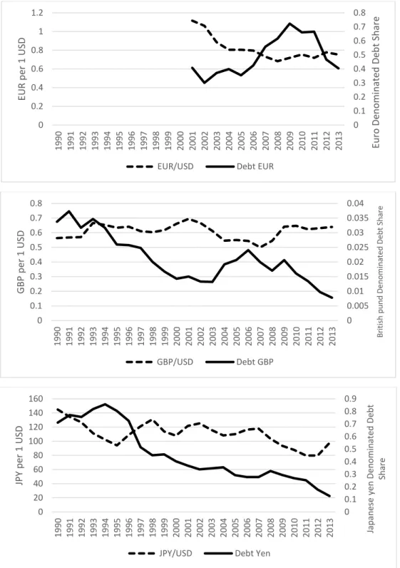
Figure 2 shows that during 1993-2013, US dollar value of Euro denominated debt share has been fluctuated in the level of 40% relative to debt share denominated in US dollar. However, the US dollar value of British pound denominated debt share falls from 3% to 1% relative to debt share denominated in US dollar, and Japanese yen denominated debt has dwindled from 60% to 15% relative to debt share denominated in US dollar.

Using time-series analysis, another preliminary test provide (i) the correlation between changes in debt share and exchange rates series, and (ii) standard deviations of the two series. This descriptive test can be observed in Table 2.

Figure 2 Foreign Currency-denominated Debt Shares and Exchange Rates Source: Own creation

0 0.1 0.2 0.3 0.4 0.5 0.6 0.7 0.8 0 0.2 0.4 0.6 0.8 1 1.2 1990 1991 1992 1993 1994 1995 1996 1997 1998 1999 2000 2001 2002 2003 2004 2005 2006 2007 2008 2009 2010 2011 2012 2013 Eu ro De n o m in at ed De b t Sh ar e EU R p er 1 USD

EUR/USD Debt EUR

0 0.005 0.01 0.015 0.02 0.025 0.03 0.035 0.04 0 0.1 0.2 0.3 0.4 0.5 0.6 0.7 0.8 1990 1991 1992 1993 1994 1995 1996 1997 1998 1999 2000 2001 2002 2003 2004 2005 2006 2007 2008 2009 2010 2011 2012 2013 B ri ti sh pu nd D eno m ina te d D ebt S ha re G BP p er 1 USD GBP/USD Debt GBP 0 0.1 0.2 0.3 0.4 0.5 0.6 0.7 0.8 0.9 0 20 40 60 80 100 120 140 160 1990 1991 1992 1993 1994 1995 1996 1997 1998 1999 2000 2001 2002 2003 2004 2005 2006 2007 2008 2009 2010 2011 2012 2013 Jap an es e ye n De n o min ate d De b t Sh are JPY p er 1 USD

Table 2 Preliminary Test

Country

Correlation Volatility Ratio

EUR GBP JPY EUR GBP JPY

Brazil 0.20 0.17 0.60 0.002 * 0.0001 * 0.33 China -0.43 * -0.23 * 0.65 -0.02 * -0.00006 * 2.37 Colombia 0.58 -0.15 * 0.53 0.004 * -0.00004 * 0.30 Egypt -0.45 * -0.41 * -0.26 * -0.02 * -0.0003 * -0.28 * Hungary -0.17 * -0.24 * 0.26 -0.02 * -0,0006 * 4.67 India -0.20 * -0.09 * -0.34 * -0.001 * -0.0001 * -0.31 * Indonesia -0.44 * -0.46 * 0.35 -0.006 * -0.0004 * 2.97 Malaysia -0.14 * 0.006 * 0.54 -0.001 * 0.00001 * 3.37 Mexico -0.55 * 0.09 0.16 -0.003 * 0.00003 * 0.12 Morocco -0.83 * 0.06 -0.72 * -0.22 * 0.000005 * -2.23 * Peru -0.002 * 0.11 0.08 -0.002 * 0.00006 * 0.09 Philippines -0.16 * -0.15 * 0.32 -0.001 * -0.00006 * 1.41 Thailand 0.04 * -0.18 * 0.57 0.00008 * -0.00006 * 6.49 Turkey -0.57 * 0.31 0.21 -0.01 * 0.0002 * 0.69 Note: Significance level at 5% is denoted as (*) and the values presented are the p-value. The null hypothesis for correlation is that the correlation between changes in exchange rates and changes in debt shares is equal to zero. The null hypothesis for volatility ratio is that changes in debt shares to the variance of the changes in exchange rates is equal to one.

Table 2 shows the preliminary test for correlation and volatility ratio. The null hypothesis for bivariate correlation is that the correlation between changes in exchange rate and changes in debt shares is equal to zero. While for volatility ratio the null hypothesis is the variance of the changes in exchange rates to variance of changes in debt shares is equal to one.

For an optimal portfolio management, change in exchange rate should not changes the US dollar value of debt denominated in these three currencies. If the US dollar value of debt changed, the portfolio value also changed and it is not optimal. Hence, for an optimal portfolio management the null hypothesis of no correlation is that the correlation between changes in debt shares and changes in exchange rates should equal to zero.

Furthermore, an optimal portfolio management should have ratio between standard deviation of the US dollar value of debt shares to the standard deviation of the corresponding exchange rates should be less than one. Changes in exchange rates must be more volatile than changes in US dollar value of debt shares.

5.2 Panel Unit Root Testing

Level First Difference Debt Euro 3.41 (0.9997) -2.47 (0.0068) * Debt GBP 6.56 (1.0000) -2.97 (0.0015) * Debt Yen 4.19 (1.0000) -3.99 (0.0000) * EUR/USD -0.96 (0.7358) -5.19 (0.0000) * GBP/USD -2.68 (0.0952) -8.65 (0.0000) * JPY/USD -2.99 (0.0511) -8.13 (0.0000) * Note: Significance level at 5% is denoted as (*), the values outside parentheses are t-statistics values, and values in parentheses are the p-value. The null hypothesis for unit root test is that variables in questions contain unit roots versus the alternative hypothesis that the variable is stationary.

From table 3 above, in the level all series show no rejection of the null hypothesis at 5% signif-icance level. However, in first difference all series show rejection to the null hypothesis. Hence, all the variables in questions are stationary in the first difference which means that they contain a unit root i.e. they are I(1).

5.3 Cointegration Testing

Table 4 Panel Cointegration Test (Pedroni (Engle-Granger based))

Debt EUR Debt GBP Debt Yen

Trend -2.37 (0.0092) * -3.91 (0.0000) * -6.18 (0.0000) * Without Trend -5.28 (0.0000) * -4.57 (0.0000) * -7.62 (0.0000) * Note: Significance level at 5% is denoted as (*), the values outside parentheses are the t-statistics values, and values in parentheses are the p-values. The null hypothesis for cointegration test is that there is no cointegrating vector in variables in question versus the alternative hypothesis that there is at least one cointegrating vector. Table 4 shows that at 5% significance level, the p-values for all debt shares are less than the significance level, therefore the null hypothesis is rejected and conclude that at least one of the series is cointegrated. Panel cointegration test using Kao-ADF (1999) method is performed to ensure that the result is valid. Kao states that his model fits with finite sample and he has eval-uated the model using Monte Carlo experiments. Since this thesis uses limited sample of foreign debt data, therefore Kao method makes the result stronger. The result of the test is as the fol-lowing:

Table 5 Panel Cointegration Test (Kao (Engle-Granger based))

Debt EUR Debt GBP Debt Yen

Without Trend -7.65 (0.0000) * -6.66 (0.0000) * -9.95 (0.0000) * Note: Significance level at 5% is denoted as (*), the values outside parentheses are the t-statistics values, and values in parentheses are the p-values. The null hypothesis for cointegration test is that there is no cointegrating vector in variables in question versus the alternative hypothesis that there is at least one cointegrating vector.

From Table 5 above, the cointegration tests using Kao method shows that the p-values for all debt shares are less than 5% significance level, therefore the results are supportive to the results from Pedroni method that all debt shares are cointegrated with related exchange rate.

5.4 Cointegrating Vectors in Panels and Reversal Time

The results of DFE with two lags and two leads can be observed in the following table:

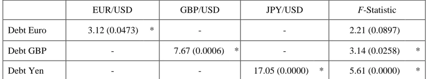
Table 6 Dynamic Fixed-effect Estimator (DFE)

EUR/USD GBP/USD JPY/USD F-Statistic

Debt Euro 3.12 (0.0473) * - - 2.21 (0.0897) Debt GBP - 7.67 (0.0006) * - 3.14 (0.0258) * Debt Yen - - 17.05 (0.0000) * 5.61 (0.0000) * Note: Significance level at 5% is denoted as (*), the values outside the parentheses are the F-Statistics values, and the values in parentheses are the p-values.

The DFE method is performed to test the robustness of cointegrating vectors in temporal period. From the Table 6 above, the results of the DFE test show that the foreign debt portfolio is not efficient shown by strong evidences of long-run relationships between debt share and respected exchange rate. The long-run relationship is observed at 5% significance level for debt share denominated in Euro, British pound, and Japanese yen. The null hypothesis of no causality is rejected in two out of three cases (Euro debt share & exchange rate is significant at 10% level) therefore respected exchange rate does Granger cause the corresponding debt share.

In order to achieve an efficient foreign debt portfolio management, we provide the simulation for how long the average time needed for debt share to reverse back to the initial position which is to keep the constant position. The calculations of the reversal time based on DFE model is applied according to Iancu (2007) as in the following table:

Year Debt EUR (Lnωij=-3.97333) Debt GBP (Lnωij=-7.06382446) Debt JPY (Lnωij=-1.67752)

LnYi,t LnYi,t-j LnYi,t-LnYi,t-j t LnYi,t LnYi,t-j LnYi,t-LnYi,t-j t LnYi,t LnYi,t-j LnYi,t-LnYi,t-j t

1990 1991 -3.2892 -3.3881 0.0989 -0.0140 -0.2598 -0.3408 0.0809 -0.0483 1992 -3.4515 -3.2892 -0.1624 0.0230 -0.2799 -0.2598 -0.0200 0.0119 1993 -3.3616 -3.4515 0.0899 -0.0127 -0.1999 -0.2799 0.0800 -0.0477 1994 -3.4508 -3.3616 -0.0892 0.0126 -0.1551 -0.1999 0.0448 -0.0267 1995 -3.6513 -3.4508 -0.2006 0.0284 -0.2192 -0.1551 -0.0641 0.0382 1996 -3.6601 -3.6513 -0.0088 0.0012 -0.3212 -0.2192 -0.1020 0.0608 1997 -3.6978 -3.6601 -0.0377 0.0053 -0.6627 -0.3212 -0.3415 0.2035 1998 -3.9121 -3.6978 -0.2143 0.0303 -0.7977 -0.6627 -0.1350 0.0805 1999 -4.0917 -3.9121 -0.1796 0.0254 -0.7819 -0.7977 0.0158 -0.0094 2000 -4.2489 -4.0917 -0.1573 0.0223 -0.9099 -0.7819 -0.1281 0.0764 2001 -4.1977 -4.2489 0.0513 -0.0073 -0.9990 -0.9099 -0.0890 0.0531 2002 -1.2015 -0.8973 -0.3042 0.0765 -4.3185 -4.1977 -0.1208 0.0171 -1.0836 -0.9990 -0.0847 0.0505 2003 -0.9910 -1.2015 0.2105 -0.0530 -4.3275 -4.3185 -0.0089 0.0013 -1.0581 -1.0836 0.0256 -0.0152 2004 -0.9194 -0.9910 0.0716 -0.0180 -3.9535 -4.3275 0.3740 -0.0529 -1.0356 -1.0581 0.0225 -0.0134 2005 -1.0365 -0.9194 -0.1171 0.0295 -3.8792 -3.9535 0.0742 -0.0105 -1.2286 -1.0356 -0.1930 0.1150 2006 -0.8573 -1.0365 0.1792 -0.0451 -3.7279 -3.8792 0.1513 -0.0214 -1.2829 -1.2286 -0.0543 0.0324 2007 -0.5821 -0.8573 0.2752 -0.0693 -3.9146 -3.7279 -0.1867 0.0264 -1.2831 -1.2829 -0.0003 0.0002