Limiting source dimensions of three-dimensional analytical point source model for solute transport

Full text

(1)Hydrology Days Proceedings 2003, 1-15. Limiting Source Dimensions of Three-Dimensional Analytical Point Source Model for Solute Transport A. Noman M. Ahsanuzzaman1 University of Oklahoma. Randall Kolar2, PhD University of Oklahoma. Musharraf Zaman3, PhD University of Oklahoma. Abstract. This article presents a criterion for limiting source dimensions of the instantaneous point source model. The source dimensions are required for applying superposition of the point sources in space to represent the non-point sources. The criterion generates less than one percent error when compared to the existing finite source model. A comparison between the existing point and the finite source models is conducted. It is found that the finite source model does not give acceptable output at all times, if series distribution is used to compute the error function. The front and tail of the concentration breakthrough curve from the finite source model shows uncharacteristic output depending on the source dimension and the distance of the observation point. On the contrary, the point source model generates smooth breakthrough curves at all time.. 1. Introduction Analytical models for solute transport are very common in groundwater modeling. Analytical models are very simple to use and less likely to produce erroneous results when compared to the numerical models. Moreover, the analytical models are very useful for validation or calibration of numerical models (Leij et al. 1991; Park and Zhan 2001; Sim and Chrysikopolous 1998). A number of analytical models for point and nonpoint sources are available at present. The analytical model for instantaneous point source in one-dimension is first presented by Crank (1956). Baetsle (1969) extended the model to three-dimensional dispersion. Later, Hunt (1978) and Sun (1996) derived the same analytical model (Baetsle 1969) 1. PhD Candidate, University of Oklahoma 1101 East 9th St. #5 Ada, OK 74820 Email: noman@ou.edu Phone: (580) 436-8587 Fax: (580) 436-8718 2. Associate Professor, University of Oklahoma. 3. Professor, University of Oklahoma.  Hydrology Days 2003.

(2) Ahsanuzzaman et al.. using different mathematical analyses. van Genuchten and Alves (1982) presented a number of analytical solutions of the one-dimensional convective-dispersive solute transport equation. Several researchers have published three-dimensional analytical models for finite or patch sources (Leij et al. 1991; Park and Zhan 2001; Sim and Chrysikopolous 1998; Cleary and Ungs 1978; Yeh 1981; Domenico 1987; Domenico and Robbins 1985; Martin-Hayden and Robbins 1997; Neville 1994; and Wexler 1992). Leij et al. (1991) has presented analytical solutions, commercially available as 3DADE (Leij and Bradford 1994), for different shapes of source in a semi-infinite domain in the direction of groundwater flow and infinite domain in the other two directions. This implies that the sources in the horizontal plane should be placed in the middle of the aquifer so that the lateral and the vertical spreading cannot reach the boundaries. Neville (1994), Cleary and Ungs (1988), Domenico (1987), Domenico and Robbins (1985), Martin-Hayden and Robbins (1997), and Wexler (1992) models are limited to constant or temporarily continuous patch sources. Park and Zhan (2001), and Sim and Chrysikopolous (1998), and Yeh (1981) considered a time dependent finite concentration source in aquifers with finite and infinite thickness. Although a number of analytical models are available, evaluation of solute transport from transient finite sources is generally conducted from the numerical models, which are widely available at present (Leij et al. 1991). Numerical models are preferred partly because the analytical models contain complex mathematical functions and often require numerical integration of the temporal term to represent continuous sources. The other advantages of the numerical models are obviously the flexibility in handling complex geology and hydraulic boundaries. However, numerical modeling warrants technical skills in setting up the boundaries of the model as well as in calibration of the model, and inefficient use of the numerical models can produce largely erroneous results. Therefore, it is always useful to use analytical models for homogeneous geology and simple hydraulic boundaries. In addition, analytical models are useful as a preliminary site assessment tool. One possible way to make the analytical models for finite sources more useful is by applying superposition of a point source model, which contains simple mathematical functions. When the advection-dispersion solute transport equation is linear (typically assumed for many applications), superposition of the point sources in space can be applied to represent finite sources (Sun 1996). With the advent of computer technology, a simple code for superposition in time and in space can be easily developed. The analytical model for instantaneous point source can be superposed in time and in space to get downgradient concentration from a finite source with transient releases. However, to apply superposition in space, the number of point sources to be superposed to represent the finite source, and the dimensions of each point source should be defined. The dimensions of each point source are critical as larger dimensions can result in erroneous estimation from the analytical point source model. One can possibly divide the finite source into a large number.  Hydrology Days 2003. 2.

(3) Limiting Source Dimensions. of point sources with very small dimensions to minimize the computational error. However, there will always be questions that what the limiting source dimension of the each point source is, and how the superposition can be optimized for minimum number of point sources. To this end, the primary objective of this study is to develop a criterion for the source dimensions of the point source model so that it gives equivalent output to the existing finite source models. In the context, a comparison between the point and the finite source models is also presented in this study.. 2. Analytical Models for Instantaneous Point Sources The advection-dispersion equation (ADE) for solute transport through saturated soil is given by Equation 1. Equation 1 is derived from conservation of mass in an infinitesimal elementary volume of the porous media. The equation is based on the assumptions that the porous media is homogeneous and isotropic, the flow is one-dimensional, and dispersion is threedimensional. Also, the solute is miscible, non-degradable, non-reactive, and non-adsorptive to the media.. ∂C ∂ 2C ∂ 2C ∂ 2C   ∂C    = − v x + + D D  +  D x y z ∂t ∂x 2 ∂y 2 ∂z 2   ∂x  . (1). where, C is the solute concentration, vx is the average fluid velocities in the x direction, t is any given time, and Dx, Dy, Dz are the hydrodynamic dispersions in the x, y and z directions, respectively. Solution (Equation 2) of the ADE (Equation 1) for instantaneous injection of solute mass at the origin as point source was first derived by Baetsle (1969). Baetsle (1969) extended Crank’s (1956) solution for onedimensional dispersion to represent three-dimensional dispersion (Equation 4.2). Hunt (1978) and Sun (1996) solved the ADE analytically and gave the same solution (Equation 2). Crank (1956), Hunt (1978), and Sun (1996) used semi-infinite boundary towards the direction of flow and infinite boundary in the lateral and in the vertical directions. C(x, y, z, t) =. M 8(π t). 3. 2.  (x - v x t )2 y2 z 2  exp− − −  4D x t 4D y t 4D z t   Dx D yDz n. (2). where, M is the mass of solute injected instantaneously at the origin at t = 0, and n is the porosity of the medium..  Hydrology Days 2003. 3.

(4) Ahsanuzzaman et al.. Crank (1956) used the generalized probability function to define concentration in one dimensional, non-advective flow domain (i.e., vx = Dy = Dz = 0 in Equation 1) as C(x, t) =. A 1 t2. exp(− x 2 /4D x t). (3). where, A is an arbitrary constant. By assuming the total amount of mass (M) diffusing in a cylinder of infinite length with unit cross-section, M is given by. M/n = ∫−∞∞ Cdx. (4). Solving Equations 3 and 4, one can get the solution for C as C(x, t) =. M. n. 2(πD x t). 1. 2.  x2   exp −  4D x t . (5). Baetsle (1969) extended Equation 5 to derive Equation 2 by considering a three-dimensional dispersive field in a moving coordinate system, moving at velocity vx towards the direction of flow. Hunt (1978) used the solution of analogous equations in heat conduction, derived by Turner (1972), to derive Equation 2. Sun (1996) used a completely analytical concept to solve the ADE (Equation 1). Sun (1996) assumed an infinitesimal spherical point mass (Equation 6) to solve the ADE in spherical coordinate system (Equation 7). Sun (1996) then converted the solution (Equation 7) to Cartesian coordinate system with the X-axis moving at velocity vx to derive Equation 2. M = 4π θ ∫0∞ Cr 2 dr C (r,t) =. M. (6). n. 8(π Dt). 3. exp( − 2. r2 ) 4Dt. (7). Solution of the ADE (Equation 1) for instantaneous cubic (finite) source of solute mass, with dimension equal to ‘LS’ at time zero, was first derived by Hunt (1978) (Equation 8). Hunt (1978) integrated the point source model (Equation 2) over the area of the finite source dimensions and applied Fourier transformation to derive Equation 8. Equation 8 gives concentration at any downgradient point (x,y,z) from the center of the source (0, 0, 0) at any.  Hydrology Days 2003. 4.

(5) Limiting Source Dimensions. given time ‘t’. Later, Domenico and Robbins (1985) presented Hunt’s (1978) equation for a parallelepiped shape source. The equation presented by Domenico and Robbins (1985) for instantaneous parallelepiped shape source incorrectly represented the parentheses before the source dimensions. The corrected form of the solution for a parallelepiped shape source is presented in Equation 10.   L  x - vx t + S 2  n C(x, y, z, t) = erf  2 Dx t 8L S 3     M.   LS erf  y + 2   2 D t y  .   y − LS   2  − erf    2 Dyt  .   x - v t − LS   x 2  − erf  2 Dx t    .    z + L S    2  erf     2 D z t   .     .   z − LS   2  − erf    2 Dz t  .     . (8). where, ‘erf’ represents the error function. The series distribution of the error function is given by,. erf ( x) =. (− 1)n x 2n+1 ∑ (π )0.5 n=0 (2n + 1) × n!) 2. ∞. (9).   X  x - vx t + S 2  n C(x, y, z, t) = erf  8X S YS Z S   2 Dx t   M.   YS erf  y + 2   2 D t y  .   y − YS   2  − erf    2 Dyt  .   x - v t − XS   x 2  − erf  2 Dxt    .    z + Z S    2  erf     2 D z t   .   z − ZS   2  − erf    2 Dzt  .          . (10). where, XS, YS, and ZS represent source dimensions along x, y, and z axis, respectively. Please note that the solute concentration at the source is equal to M/(nXSYSZS).. 3. Comparison of the Instantaneous Point and Finite Source Models In order to compare the instantaneous point source and the finite source models, both models are run for the same datasets. A software program is developed to run the models and generate breakthrough curves at any given observation point. Four longitudinal source dimensions (1.5, 15,.  Hydrology Days 2003. 5.

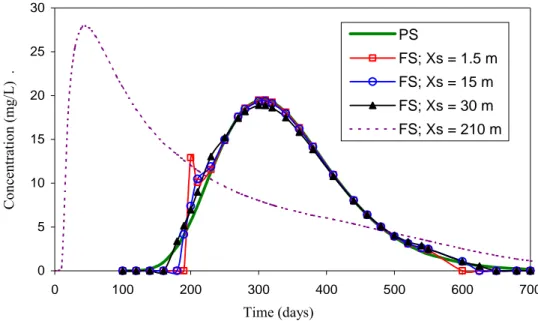
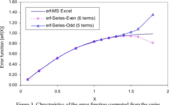
(6) Ahsanuzzaman et al.. 30, and 210 m) are used to compare the models for different source sizes. The lateral and the vertical source dimensions are considered to be 1.5 and 0.3 m, respectively. It should be noted that for all source dimensions, the total mass input (M) is kept constant at 100 kg and the source concentrations (C0) is changed proportionally. Other input data used in the simulation are groundwater velocity (vx) equal to 0.36 m day-1, and longitudinal, lateral, and vertical dispersivities equal to 4.5, 0.45, and 0.045 m, respectively. Molecular diffusion is assumed to be negligible, as the common value from literature [1.0E-09 m2 day-1 (Cussler 1997; Fetter 1999)] is about 200 times smaller than the vertical dispersion (αzvx) for the selected inputs. Figure 1 and 2 show the breakthrough curves generated from both the point source (PS) and the finite source (FS) models. The breakthrough curves are generated for two downgradient observation points at 120 m (Figure 1) and 300 m (Figure 2) away from the center of the source along the centerline of the plume. It is evident from both figures that the point source model generates smooth breakthrough curve, while the breakthrough curves from the finite source model are not smooth at all time. Uncharacteristic output is found at the front and the tail of the breakthrough curves from the finite source model, while almost identical outputs are found from both models at the middle section of the breakthrough curves. The uncharacteristic output for the FS model results due to the use of a truncated series distribution for the error function (Equation 9). Figure 3 illustrates the characteristics of the error function computed from the series distribution with odd (5 terms) and even (6 terms) number of terms. It is found that a truncated series distribution is not good when the independent variable (x) is greater than 1.2 i.e., when the error function is greater than 0.91. The truncated series distribution shows sharp drop from the actual value of the error function (‘erf-MS Excel’) when even number of terms are used, while sharp rise is observed when odd number of terms are used (see Figure 3). The FS model is very sensitive to the computational method of the error function, as it uses subtraction of the error functions for each dimension (see Equation 10). When the source dimensions are small, the calculation of the error function needs to be highly accurate to get acceptable output from the FS model, as the source dimensions cause the difference in the error functions for each dimension (see Equation 10). This is also evident from Figures 1 and 2, where the largest source dimension (XS = 210 m) does not show any uncharacteristic output, while the others do. Figures 1 and 2 are generated for error functions computed from odd number of terms (5 terms) in the series distribution. For even number of terms (6 terms), the first dataset of Figure 1 is reproduced in Figure 4. It is found that for even number of terms the front and tail of the breakthrough curve show unrealistic concentrations that extend in the negative direction, while the middle section matches well with the point source model (see Figure 4). If the negative concentrations resulting from the error function with even number of terms are masked to zero concentration by the computer code, the break through curve is more acceptable than that for odd number of terms in the series distribution (see Figure 5). Therefore, it is suggested to use.  Hydrology Days 2003. 6.

(7) Limiting Source Dimensions. even number of terms in the series distribution of error function and mask the output negative concentrations to zero. On the other hand, an optimized code for the error function similar to MS-Excel would obviously be ideal for the finite source model. However, such optimized code for the error function may not be readily available. It can be concluded from the observations that the instantaneous finite source model does not give acceptable output at all times (uncharacteristic output at the front and the tail of the breakthrough curves), if a truncated series distribution is used to compute the error function. The finite source model gives reasonable output at the front and the tail of the break through curve, if an even number of terms is used in the series distribution of the error function and the negative concentrations, if any, are masked to a zero value. In comparison to the finite source model, the point source model, which is more popular than the finite source model, generates smooth or stable breakthrough curve at all given times. Moreover, it requires much simpler mathematical function than the finite source model, and could be easily converted into a computer code. However, to achieve acceptable output from the point source model, the source dimensions need to be selected carefully so that the middle section of the breakthrough curve matches to that of the finite source model. The criterion for the point and the finite source models to generate equivalent concentration are derived in the following section.. 4. Limiting Source Dimensions for Analytical Point Source Model For the analytical point source and the finite source models to present equivalent concentration at the center of the plume i.e., at (vxt, 0,0), Equations 2 and 10 should be equal. Equation 11 represents the condition when the point source and the finite source models are equivalent at the center of the plume. Considering the solution technique used by Baetsle (1969), who extended Crank’s (1956) solution for one-dimensional model (Equation 5) into three-dimensions, Equation 11 can be rewritten in three equations (Equations 12, 13, and 14) representing probability density functions contributed from each dimension. 1 2 π Dx t. ×. 1 2 π Dyt. ×. 1 2 π Dzt.   X S  1   2  × 1 = erf   X S   2 D x t  YS   .  Hydrology Days 2003.   YS  erf  2  × 1   2 D t  Z S y    . 7.   ZS  erf  2    2 D t  z    . (11).

(8) Ahsanuzzaman et al..   X S  1   2  erf =   2 π D x t X S   2 D x t    . (12).   YS   1   2 erf  =   2 π D y t YS 2 D y t     . (13).   ZS   1   2 erf =   2 π D z t Z S   2 D z t    . (14). 1. 1. 1. Replacing the error function by its series distribution (Equation 9), Equation 11 can be rewritten as, 1 2 π Dx t. =. 1 XS. 3 5  X S    XS   XS  2  2 − 1  2  + 1  2  − .. (15)        π  2 D x t  3 ⋅ 1!  2 D x t  5 ⋅ 2!  2 D x t         . It is evident from Equation 15 that the left side of the equation is exactly equal to the first term of the right side. Therefore, it can be concluded that the analytical point source model is equivalent to the analytical finite source model when the error function in the finite source model is equal to the linear term of its series distribution i.e., when,   X S   XS  erf  2  = 2  2       π  2 Dxt  2 D x t       . (16). and similarly when   YS  YS   erf  2  = 2  2      2 D t  π  2 Dyt   y      . (17).   ZS  ZS   erf  2  = 2  2      2 D t  π  2 Dzt  z       . (18).  Hydrology Days 2003. 8.

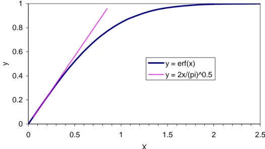
(9) Limiting Source Dimensions. Graphical representation of the error function (Figure 6) shows that the error function is linearly proportional to the independent variable when the latter is very small. It is evident that the point source model follows the straight line in Figure 6, while the finite source model follows the non-linear line (i.e., the error function). Therefore, the point source and the finite source model should generate equivalent result as long as the error function in the finite source model varies linearly. From trial and error, it is found that Equation 16 to 18 satisfy with less than 1 percent error when,  X S   YS   ZS   2 or ,  2 or ,  2  ≤ 0.17        2 Dx t   2 Dy t   2 Dz t       . (19). Equation 19 can be used to find the dimension of a source (XS, YS, and ZS) for the analytical point source model. Since the comparison is at the center of the plume, the variable ‘t’ can be replaced by ‘x/vx’ in Equation 19. Since the error function is about 1 percent less than the independent variable when the latter is equal to 0.17, each source dimension obtained from Equation 19 produces 1 percent error for the point source model. Therefore, the total error resulted from the point source model with source dimensions obtained from Equation 19 is about 3 percent [= (1.013 –1)×100]. In order to reduce the total error to 1 percent, the error produced by each source dimension should be 0.33 percent [= (1.011/3 –1)×100]; For the error function to produce 0.33 percent smaller value than the independent variable, the latter has to be 0.10. Therefore, for about 1 percent total error from the point source model, the source dimensions are given by Equation 20.          ZS   YS  XS      2 2 2  ≤ 0.10  or ,  or ,   2 D x  2 D x  2 D x  z y x  v x   v x   v x  . (20). Equation 20 is verified by comparing the point and the finite source model outputs for the source dimensions from that equation. For an observation point 120 m away from the center of the source, the limiting source dimensions from Equation 20 are 9.44, 2.98, and 0.944 m along x, y, and z directions, respectively. Keeping all other inputs equal to those stated earlier, the simulation shows that the finite source model gives a maximum concentration of 19.36 mg/L while, the same for the point source model is 19.56 mg/L, resulting about 1 percent error in calculating the maximum concentration..  Hydrology Days 2003. 9.

(10) Ahsanuzzaman et al.. 5. Conclusion The primary objective of this study is to develop a criterion for the source dimensions of the point source model so that it gives equivalent output to the existing finite source models. Finite source dimensions are required for applying superposition (in space) of the point source model to represent nonpoint sources. In the process of developing the criterion for source dimensions, a comparison between the point and the finite source models is conducted. It is found that the instantaneous finite source model does not give acceptable output at all times if series distribution is used to compute the error function. The front and tail of the concentration breakthrough curves from the finite source model show uncharacteristic output, depending on the representation of the error function and the source dimension and the distance of the observation point. The finite source model gives reasonably acceptable output at the front and the tail of the break through curve, if an even number of terms are used in the series distribution of the error function and the negative concentrations, if any, are masked to a zero value. In comparison to the finite source model, the point source model, which is more popular than the finite source model (with series distribution of the error function), generates smooth or stable breakthrough curve at all given times. Superposition of the point source model with acceptable source dimensions is computationally simpler than superposing the finite source model, since the point source model does not rely on an error function that, lacking optimized libraries, must be represented with a truncated Taylor series; thus, for convenient analyses, point source models can be easily converted into a computer code. A criterion for the source dimensions of the point source model is developed (Equation 19) by comparing the finite source model by Domenico and Robbins (1985) with the point source model by Baetsle (1969). The criterion (Equation 19) generates less than one percent error when compared to the existing finite source model.. 6. References Baetsle, L. H., 1969: Migration of Radionuclides in Porous Media, Progress in Nuclear Energy, Series XII, Health Physics, ed. A. M. F. Duhamel Pergamon Press, Elmsford, New York, 707-730. Cleary, R. W., and M. J. Ungs, 1978: Analytical Methods for Ground Water Pollution and Hydrology, Water Resources Program Report: 78-WR-15, Department of Civil Engineering, Princeton University, Princeton, New Jersey. Crank, J., 1956: The Mathematics of Diffusion, Oxford University Press Inc., New York, 414 p..  Hydrology Days 2003. 10.

(11) Limiting Source Dimensions. Cussler, E. L., 1997: Diffusion Mass Transfer in Fluid Systems, 2nd Edition, Cambridge University Press, UK, 580 p. Domenico, P. A., 1987: An Analytical Model for Multidimensional Transport of a Decaying Contaminant Species, Journal of Hydrogeology, 91:49-58. Domenico, P. A., and G. A. Robbins, 1985: A New Method of Contaminant Plume Analysis, Ground Water, 23(4): 51-59. Fetter, C. W., 1999: Contaminant Hydrogeology, 2nd Edition, Prentice Hall, New Jersey, 500 p. Hunt, B., 1978: Dispersive Sources in Uniform Ground-Water Flow, Journal of the Hydraulics Division, Proceeding of American Society of Civil Engineering, 104:75-85. Leij, F. J., and S. A. Bradford, 1994: 3DADE: A Computer Code for Evaluating Three-Dimensional Equilibrium Solute Transport in Porous Media, Version 1.0. Research Report No. 134, U.S. Salinity Laboratory, USDA, ARS, Riverside, California. Leij, F. J., T. H. Skaggs, and M. Th. van Genuchten, 1991: Analytical Solutions for Solute Transport in Three-Dimensional Semi-Infinite Porous Media, Water Resources Research, 27(10): 2719-2733. Martin-Hayden, J. M., and G. A. Robbins, 1997: Plume Distortion and Apparent Attenuation Due to Concentration Averaging in Monitoring Wells, Ground Water, 35(2): 339-346. Morris D. A., and A. I. Johnson, 1967: Summary of Hydrologic and Physical Properties of Rock and Soil Materials as Analyzed by the Hydrogeologic Laboratory of the U. S. Geological Survey, U.S. Geological Survey Water Supply Paper 1839-D. Neville, C. J., 1994: Compilation of Analytical Solutions for Solute Transport in Uniform Flow, S. S. Papadopulos & Associates, Bethesda, Maryland. Park. E., and H. Zhan, 2001: Analytical Solutions of Contaminant Transport from Finite One-, Two-, Three-Dimensional Sources in a Finite-Thickness, Journal of Contaminant Hydrology, 53: 41-61. Sim, Y., and C. V. Chrysikopoulos, 1999: Analytical Solutions for Solute Transport in Saturated Porous Media with Semi-Infinite or Finite Thickness, Advances in Water Resources, 22(5): 507-519..  Hydrology Days 2003. 11.

(12) Ahsanuzzaman et al.. Sun, N. Z., 1996: Mathematical Modeling of Groundwater Pollution, Springer, New York, 377 p. Turner, G. A., 1972: Heat and Concentration Waves, Academic Press, New York, New York. van Genuchten, M. Th., and W. J. Alves, 1982: Analytical Solutions of the One-Dimensional Convective-Dispersive Solute Transport Equation, U. S. Department of Agriculture, Technical Bulletin No. 1661, U. S. Salinity Laboratory, Riverside, California, 151p. Wexler, E. J., 1992: Analytical Solutions for Chemical Transport in GroundWater Systems with Uniform Flow, Book 3, Chapter B7, U. S. Geological Survey, Denver, Colorado, 190 p. Yeh, G. T., 1981: AT123D: Analytical Transient One-, Two-, and ThreeDimensional Simulation of Waste Transport in an Aquifer System, Report ORNL-5602, Oak Ridge National Laboratory, Oak Ridge, Tennessee..  Hydrology Days 2003. 12.

(13) Limiting Source Dimensions. 30. PS Concentration (mg/L) .. 25. FS; Xs = 1.5 m FS; Xs = 15 m. 20. FS; Xs = 30 m FS; Xs = 210 m. 15 10 5 0 0. 100. 200. 300. 400. 500. 600. 700. Time (days). Figure 1. Breakthrough curves for point (PS) and finite (FS) source models at x = 120 m. Concentration (mg/L) .. 5. PS FS; Xs = 1.5 m FS; Xs = 15 m FS; Xs = 30 m FS; Xs = 210 m. 4. 3. 2. 1. 0 300. 500. 700. 900. 1100. 1300. 1500. Time (days). Figure 2. Breakthrough curves for point (PS) and finite (FS) source models at x = 300 m.  Hydrology Days 2003. 13. 1700.

(14) Ahsanuzzaman et al.. 1.60. erf-MS Excel. 1.40. Error function [erf(X)] .. erf-Series-Even (6 terms) 1.20. erf-Series-Odd (5 terms). 1.00 0.80 0.60 0.40 0.20 0.00 0. 0.5. 1. 1.5. 2. X. Figure 3. Chracteristics of the error function computed from the series ditribution. 100. Concentration (mg/L) .. 0 -100 -200. FS (for 6 terms). -300. Point Source. -400 -500 -600 100. 200. 300. 400. 500. 600. 700. 800. Time (days). Figure 4. Breakthough curves for point and finite source (Xs = 1.5 m) models at x = 120 m.  Hydrology Days 2003. 14.

(15) Limiting Source Dimensions. 25 FS (for 6 terms). Concentration (mg/L) .. 20. Point Source FS (for 5 terms). 15. 10. 5. 0 100. 200. 300. 400. 500. 600. 700. 800. Time (days). Figure 5. Breakthough curves at x = 120 m for finite source (Xs = 1.5 m) with even and odd number of terms in the series distribution of the error function. 1 0.8 0.6 y. y = erf(x) y = 2x/(pi)^0.5. 0.4 0.2 0 0. 0.5. 1. 1.5. 2. X. Figure 6. Graphical representation of the error function.  Hydrology Days 2003. 15. 2.5.

(16)

No results found